warwick.ac.uk/lib-publications
Original citation:
Truong, Dinh Quang, Marco, James, Greenwood, David, Ahn, Kyoung Kwan and Yoon, Yong
Il. (2018) Data-based predictive hybrid driven control for a class of imperfect networked
systems. IEEE Transactions on Industrial Informatics .
Permanent WRAP URL:
http://wrap.warwick.ac.uk/98227
Copyright and reuse:
The Warwick Research Archive Portal (WRAP) makes this work by researchers of the
University of Warwick available open access under the following conditions. Copyright ©
and all moral rights to the version of the paper presented here belong to the individual
author(s) and/or other copyright owners. To the extent reasonable and practicable the
material made available in WRAP has been checked for eligibility before being made
available.
Copies of full items can be used for personal research or study, educational, or not-for profit
purposes without prior permission or charge. Provided that the authors, title and full
bibliographic details are credited, a hyperlink and/or URL is given for the original metadata
page and the content is not changed in any way.
Publisher’s statement:
© 2017 IEEE. Personal use of this material is permitted. Permission from IEEE must be
obtained for all other uses, in any current or future media, including reprinting
/republishing this material for advertising or promotional purposes, creating new collective
works, for resale or redistribution to servers or lists, or reuse of any copyrighted component
of this work in other works.
A note on versions:
The version presented here may differ from the published version or, version of record, if
you wish to cite this item you are advised to consult the publisher’s version. Please see the
‘permanent WRAP url’ above for details on accessing the published version and note that
access may require a subscription.
Abstract—A data-based predictive hybrid driven control (DPHDC) approach is presented for a class of networked
systems compromising both computation and
communication delays, packet dropouts and disturbances. First, network problems are classified in a generic way which is used to design a network problem detector (NPD) capable of detecting online current delays and packet
dropouts. Second, a single-variable first-order
proportional-integral (PI) -based adaptive grey model (PIAGM(1,1)) is designed to predict future network problems and, to predict system disturbances. Third, a hybrid driven scheme integrated an optimal small buffer (OSB) is constructed to allow the system to operate without any interrupts due to large delays or packet dropouts. Furthermore, the OSB size is online optimized using adaptive grey fuzzy cognitive map technique. Forth, a prediction-based model-free adaptive controller (PMFAC) is developed to compensate for network problems. The DPHDC stability is theoretically proved while its effectiveness is demonstrated through a case study.
Index Terms— Networked control system, time delays, packet dropouts, prediction, model free, stability.
I. INTRODUCTION
ECENTLY with the rapid development of networking technologies, network-based remote control gains more and more attention due to its advantages over the traditional wiring control. However because of computation and communication resources restriction, time delay and packet
dropout are two critical and unavoidable factors existing in any networked control system (NCS). Only a small time delay can deteriorate the control performance and, even worse, cause the instability [1]–[3].
To address stability of NCSs with communication delays, many studies were carried out in which the controller designs were depended on assumptions that the time delay was constant [4], was bounded [2], [5]–[7], had a probability distribution function [8], or was represented based on time delay analyses [9], [10]. For NCSs with large delays, control concepts based on variable sampling periods using neural network or prediction theories were adopted [11]–[13]. Nevertheless, the observation of real delay data to train and construct the NCSs was not appropriately discussed. To solve this problem, a variable sampling period control concept for systems containing both random computation and communication delays has been developed and validated [3].
To deal with NCSs compromising both time delays and packet dropouts, many important methodologies, such as predictive control [14]–[16], adaptive control [17], hybrid control [18], robust state feedback control [19]–[21], and model predictive control (MPC) [22], were proposed. The concept of model based on the updating instants was carefully considered and implemented to derive the controllers in [19], [20]. Additionally, the network delays were presented in the general form and bounded by both upper and lower limits to reduce the conservatism problem. To minimize the communication effort as well as to improve the energy efficiency of NCSs, a robust state feedback control approach based on a so-called self-triggered sampling scheme was suggested [21]. To tackle both system state with network problems and tracking error, an extended form of MPC has been introduced in [22]. By using these techniques, although the NCS performances were remarkably improved over the traditional techniques, delays and packet dropouts were assumed to be priorly known and bounded. Another trend is known as control based on efficient networks with adaptive buffers or with compensation strategy [23], [24]. Though these methods could achieved good control results, the applicability may be limited because of the complex network designs. Furthermore, the uses of fixed sampling period and dynamic buffers with large sizes at both channels could limit the control performances. As a feasible solution for these problems, a robust variable sampling period control approach (RVSPC) [25] has been proposed. Its controllability
Data-Based Predictive Hybrid Driven Control
for A Class of Imperfect Networked Systems
Truong Q. Dinh,
Member
,
IEEE
, James Marco, David Greenwood,
Kyoung K. Ahn,
Member
,
IEEE
, and Jong I. Yoon
R
Manuscript received August 1st, 2017; revised December 9th, 2017;
accepted December 31st, 2017. This work was supported by Innovate
UK through the Agile Power Management System (APMS), project number: 102437, in collaboration with the WMG Centre of High Value Manufacturing (HVM), Babcock and Potenza, and the Korea Institute of Energy Technology Evaluation and Planning (KETEP) and the Ministry of Trade, Industry & Energy (MOTIE) of Korea (No. 20162020107450). T. Q. Dinh, J. Marco and D. Greenwood are with the Warwick Manufacturing Group (WMG), University of Warwick, Coventry, UK (email: [email protected]; [email protected]; corresponding author to provide phone: +44-24-765-74902; e-mail: [email protected];).
K. K. Ahn is with the School of Mechanical Engineering, University of Ulsan, Namgu Muger2dong, Ulsan 680-749, Korea (email: [email protected])
has been clearly proven through both simulations and real-time experiments. However, for a NCS with large delays and/or high packet dropout ratio, the RVSPC performance may be degraded when the driving commands and sensing signals are long delayed/dropped. Recently, this issue has been effectively tackled by the improved version of [25], called robust predictive control (RPC) using the adaptive buffer [26]. The main limitation still exists in either the RVSPC or RPC is acknowledged that the state feedback control unit is basically designed for a well-defined networked linear system which is actually not easy to be achieved. Thanks to the development of model-free control [27], this advanced technology is successful utilized to construct NCSs with the good adaptability [28]–[30]. Nevertheless, these control schemes remain some open problems. The network problems are assumed to be bounded within a pre-defined maximum round trip time delay which is difficult to be determined in practice. The large delay bound also leads to the slow convergence speed. Additionally due to the lack of clock synchronization between the controller and plant sides, the desired task must be given only at the plant side while it is normally given at the controller side in actual remote applications.
This paper, therefore, aims to address all the problems remained in [25], [26] and [28]–[30] by introducing a data-based predictive hybrid driven control (DPHDC) approach for a class of networked control systems including both the three delay components and packet dropouts. The main contributions of this DPHDC can be expressed as:
1) Using results in [26], delays and packet dropouts are accurately detected online using a network problem detector (NPD) based on a clear definition of network problems. Using the NPD outputs, a single-variable first-order PI-based adaptive grey model (PIAGM(1,1)) is implemented to forecast precisely future network problems and system disturbances.
2) Continue with the concept of hybrid driven scheme integrated an adaptive buffer [26] to operate the system smoothly over the imperfect network, in this study an optimal small buffer (OSB) is first time introduced. The OSB size is online optimized using the estimated packet dropouts and a novel adaptive grey fuzzy cognitive map (AGFCM). Therefore, the OSB is sufficiently constructed to compensate packet
dropouts on the forward channel.
3) A prediction-based model-free adaptive controller (PMFAC) is newly developed to ensure the robust performance disregarding the delays and packet dropouts:
- Different from [25], [26], the controller is designed based on only a small data of the control input and system response, without requiring knowledge on the state-space model. - Different from [28]–[30], the fixed constraint to design the robust control input is replaced with a time-variant constraint using the PIAGM(1,1) outputs. Consequently, convergence speed is effectively improved.
- Different from the previous studies, here the system is not affected by the large delays or high packet dropout ratio due to the use of hybrid driven scheme and OSB. A s-step-ahead control technique is used to produce a dynamic vector of the control inputs according to the buffer size.
4) Lyapunov stability conditions are invoked in the control design to guarantee the stability. Effectiveness of the proposed approach is demonstrated through a real-time case study.
II. PROBLEM DESCRIPTION
Without loss of generality, the followings are presented for a multi-input-single-output (MISO) discrete-time nonlinear system with non-uniform sampling states. A system with multiple outputs using the proposed control technique can be directly constructed from the proposed MISO form. The system plant output denoted by y can be then described as:
1
( ( ),..., ( y), ( ),..., ( U))y k f y k y k l U k U k l (1) where k denotes the timestamp at working step kth; y R 1;
( ) mu
U k R is the control input vector; f(*) is an unknown nonlinear function; lyand lU are unknown orders.
To build the free-model adaptive control (MFAC) for system (1), two following assumptions are made [27]:
Assumption 1: the partial derivative of function f(*) in (1) with respect to the control input u(k) is continuous.
Assumption 2: there is a positive constant b such that system (1) is generalized Lipschitz,y k
1
b U k
, for any k,( 1) ( 1) ( ), ( ) ( ) ( 1) 0
y k y k y k U k U k U k
.
Tasks (Algorithm 2 & Algorithm 3 – Step 1, 2)PMFAC
PIAGM1(1,1)
(Algorithm 1)
OSB
(Algorithm
3 – Step 3) Actuators
Sensors
tca(k) S ca(k)
tsc(k) Ssc(k)
Timestamps
MCU
y(k) yr(k)
DPHDC (PC)
Plant
Network
{TA} {TC}
yND(k) ^
PIAGM2(1,1)
(Algorithm 1)
tsc(k) ^
AGFCM
(Eqs (44)~(51))
OSB Size
(Eq (52))
NPD
(Eq (6)) tca
(k)
tsc(k) pca(k) psc(k)
tcom(k)
pca(k) psc(k) αs(k+1) bOSB(k+1) p^ca(k)
y*(k) y*(k) yPMFAC(k)
(Eq (2))
^
Real-time & Timestamps
U(k)
y TA(k) {TA}
{U} bOSB(k+1)
{TA} {U}
bOSB(k+1)
[image:3.595.125.478.85.254.2]yr(k)
MCU
Plant
DPHDC
t
t
t
(0) (1) (2) (3) (4)
(0)
(0) (1) (2) (3) (4)
(1) (2) (3)
(1)
ca t
(1)
sc t
(2)
ca
t tca(3)
(2)
sc t
(2)
com
t tcom(3)
(1) 0
com t
Fig. 2. Working principle of NPD.
Based on Assumptions 1 and 2, system (1) can be represented in a compacted form dynamic linearization:
( 1) T( ) ( )
y k k U k
(2)
Thus, the incremental control algorithm is derived for system (1) using the MFAC theory [27] as follows:
2
ˆ
( 1)( ( ) ( 1) ( 1))
ˆ( ) ˆ( 1)
( 1)
T
U k y k k U k
k k
U k
(3)
ˆ( ) ˆ(0) if ˆ( ) , or ( 1)
( ( ) { ( )}; ( ) { ( )}; 1,..., )
i i i i
i i u
k k u k
U k u k k k i m
(4)
2ˆ
1 ,
ˆ
r k
U k G k y k y k G k
k
(5)
where yr(k+1) is the tracking target of y(k); ˆ( )
i k is the estimation of ( )i k with initial value ˆi(0); , are the step-sizes which are normally set within (0,1] ; , are the weight factors; is a small positive constant.
Definition 1: the problems in a network are defined as:
Communication delays in forward and backward channels are in turn denoted atcaandtsc. Two threshold values,
and
ca sc
t t , are defined to classify small and large delays. A large delay is treated as a packet dropout:
( ) or ( ) Small delay ( ) or ( ) Packet dropout
ca ca sc sc
ca ca sc sc
k k
k k
t t t t
t t t t
(6)
A packet disorder is also considered as a packet dropout.
“Virtual” switches, Sca and Ssc, are in turn used to represent
the packet dropouts in the forward and backward channels.
Sca (Ssc) is opened (or 1) once a packet dropout event exists.
A set of continuous packet dropouts at timestamp kth is
denoted as pca(k) or psc(k).
The computation delay,tcom, is bounded, tcom( )k tcom. The objective is to develop a networked control scheme of system (1) using the DPHDC approach in which the network problems are classified using Definition 1.
III. DATA-BASED PREDICTIVE HYBRID DRIVEN CONTROL
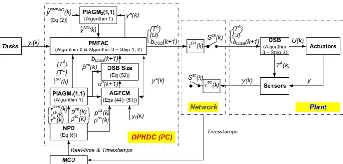
Architecture of a NCS using the DPHDC approach is depicted in Fig. 1. The system plant including a number of
actuators and sensors are driven by the DPHDC, for example, embedded in a personal computer (PC), via the network to follow given tasks. The network is with two modules attached to the controller and plant sides while the desired tasks consist of a main task to control the plant (1) using the DPHDC and other execution tasks, which could cause computation delays. Additionally, a micro control unit (MCU) is employed to equip with the NCS in order to measure the system run time.
Remark 1: The DPHDC approach is developed for system (1) over an imperfect network with following functionalities:
The NPD based on Definition 1 and the MCU output is used to detect online precisely the network problems.
The PIAGM(1,1) with prediction step size sk employs the
NPD outputs to predict the sk-step ahead network problems.
The OSB buffer is only placed at the plant side. This buffer size, bOSB, is online regulated using the AGFCM based on the
network problems and the system tracking performance.
Both the controller, sensors and actuators are hybrid time-event-driven. They are event driven when there exist only small delays; otherwise, they are time driven. The sensors and actuators are synchronous.
The PMFAC is to compensate for both the network problems classified by Definition 1 and the impacts of disturbances. According to the OSB size, bOSB, a vector of control inputs
are derived and sent to the OSB to guarantee the robust tracking performance of the actuators.
A. NPD Detector
Remark 2: From Remark 1 to construct the NPD, first, the MCU is selected as PIC18F4620 from Microchip equipped with the 4-MHz oscillator [3] to function as a reference clock to measure the real time and; second, timestamp-based detection logics developed through [25], [26], [31] are used to detect the system delays. As analyzed in [3], time resolution of the reference clock using the MCU is50s. The MCU is connected to the DPHDC-embedded PC through a PCI card [3] and, therefore, their communication delay is neglected. The delay detection principle is depicted in Fig. 2. Once system is started, an activation flag is sent from the DPHDC - MCU to the plant to activate a clock at the plant side to support the detection of forward communication delay. For the synchronization of the clocks between the MCU and plant, the first delay between the MCU and plant,tca(1), is determined using the well-known IEEE 1588-based precition time protocol, timestamps and the assumption that the forward and backward transport delay at the beginning of system operation is symetric [32], [33]. Here, the clock frequency deviation of the crystal oscillators used in the NCS are not considered. This impact on the clock synchronization can be effectively compensated using the clock model presented in [33].
From Remark 2 and Definition 1, for each working step, the NPD detects accurately the current network states with a delay set,tca( ),k tsc( )k andtcom( )k , and a set of continuous packet dropouts, pca(k) and psc(k).
B. PIAGM(1,1) Predictor and Hybrid Driven Method
while requiring only a few historical data about the predicted object [3], [25], [26], [34], [35].
Remark 3:In this study, the PIAGM(1,1) is constructed based on the general model - PINNGM(1,N) which has been successfully developed in [26]. The PIAGM(1,1) is therefore setup in the efficient way using an adaptive weight which is online regulated by a simple PI-type neural network with respect to the prediction error minimization. The robust prediction is guaranteed by a Lyapunov stability condition.
From the DPHDC architecture and Remark 1, the first PIAGM, PIAGM1(1,1), uses the historical data of network
problems (come from the NPD) to perform the sk-step-ahead
prediction of network delays, ˆca( ),ˆsc( )
s s
k i k i
t t and
ˆcom(k is),
t and packet dropouts, ˆpca(k i s) andpˆsc(k i s) in which is=2,...,sk, sk is the smallest value satisfying:
ˆ ˆ ˆ
(pca(k2) 0) [( pca(k i s 1) 0) ( pca(k i s) 0)]. For a coming step (k+1)th, using Definition 1 and the
PIAGM1(1,1) outputs, the hybrid time-event driven scheme can
be expressed through dynamic sampling rates, TC(k+1) and TA(k+1), for the controller and plant sides, respectively:
ˆ ˆ ˆ
1 1 min 1 , min 1 ,
ˆ ˆ ˆ
1 min , 1 min 1 ,
C com ca ca sc sc A sc sc com ca ca
T k k k k
T k k k k
t t t t t
t t t t t
(7)
In addition, once a package loss is detected on the backward channel, the PIAGM is applied (denoted as PIAGM2(1,1)) to
estimate the current impact of noises and disturbances on the system performance, ˆyND( )k . The historical data of system disturbances is the set of time-series differences between last values of the actual system response and the corresponding system response which is calculated based on (2) (denoted as
ˆPMFAC)
y . The estimated disturbance impact is then fed into the PMFAC to speed up the convergence speed.
C. OSB Buffer
Without any buffer, the controlled system is difficult to follow the desired goal when there is a large numbers of packet dropouts. On the contrary, the control performance becomes poor when using a large size buffer. Since, the key concept is to regulate online the OSB size,bOSB(k 1) sk, to store enough commands to drive the actuators during a period consisting of
ˆ (ca k)
p k s continuous packet dropouts.
D. PMFAC Controller
The PMFAC takes part in driving the actuators to reach the desired targets based on Remark 1:
For each step defined by the hybrid time-event driven method (TC(k)) and based on OSB size,a set of the control
inputs are generated for the next bOSB steps using an iterative
estimation scheme.
Actual and estimated time delay factors and estimated disturbance impacts are invoked into the controller design process to compensate for these problems and, therefore, to ensure the stability.
IV. PIAGM(1,1)MODEL A. PIAGM(1,1) Design
Remark 4:Any random data set of a predicted object, yobj,
can be converted into a grey sequence which satisfies both the grey checking conditions using the cubic spline interpolation (SP, see Appendix A) and two non-negative additive factors, c1
and c2, derived by Theorem 1 in [25]. Next using [26], the
PIAGM(1,1) model with the adaptive weight is constructed. Based on Remark 4, the prediction procedure for an object,
yobj, using the PIAGM(1,1) can be expressed as follows: Algorithm 1 PIAGM(1,1) Model to Predict An Object yobj
Step 1: For any object with a data sequence
1
{ ( ),..., ( )}( 4) obj obj O obj Om
Y y t y t m , the raw input grey sequence,Yraw{yraw( ),...,t1 yraw( )}(tn n4) , is derived as
0
0
1 0
, ,
1,...,raw i i obj i i obj i
y t y t SP Y t i n (8)
where 0 i
is the activating factor following Remark 4; The input grey sequence is then computed as
0 0 0 0
1 2
{ ( ), ( ),..., ( )} 0;n 4
y y t y t y t n (9)
where 0
1 2
( )i raw( )i ;
y t y t c c
Step 2: Generate a new series y(1) by accumulating y(0):
1 0 1 1 2 1 , 1,..., ; kk i i i
k
obj i i
i
y t y t t k n
y t c c t
(10)Step 3: Define a background series z(1) as
1
1
1
2
1
1 ; 2,...,
k k k k k
z t w t y t w t y t k n (11)
1 1 1 2 2
1
2 1 1 2 1 2
( ) 0.5 1 ( ) 1 1 ( )
( ) 0.5 1 1 ( ) 1 ( )
A A
k k k
A A
k k k
w t w t w t
w t w t w t
(12)
where 0 A( ) 1 k
w t
is the adaptive factor; { , 1 2} is the set
of activated factors and given as
0 0 1 1 0 0 1 2 1 1{1,0},IF : ;
{ , } {1,1},IF : ;
{0,1},Others;
raw k k raw k obj k
raw k obj k raw k k
y t SP t y t y t
y t y t y t SP t
(13)
Step 4: Establish the grey differential equation: 0
1
k k
y t az t b (14)
By employing the least square estimation [25], one has:
1
ˆ
ˆ ˆ T ( T ) T ab a b B B B Y
(15)
1 0 2 2 1 0 1 , ; 1 n nz t y t
B Y
z t y t
Step 5: The PIAGM(1,1) prediction is then setup as
0
1 2
1
1 1ˆ ˆ ( ) ( )
ˆ ;
ˆ
1 ( )
k k k
k
k k
b a w t w t y t y t
w t a t
(16)
Step 6: Produce the sk-step-ahead prediction yobj (at step
(k+sk)th) based on (9) and (16):
0
0
0
1 2
ˆobj k ˆraw k sk ˆ k sk .
at the coming step to optimize the factor wA(t
k+1) and return to
Step 1; Otherwise, terminate the procedure.
B. Prediction Stability Analysis
The prediction using Algorithm 1 can be considered as a closed-loop tracking control problem in which the ‘control input’ A( )
k
w t needs to be designed to ensure the ‘system response’ˆ ( 0 )
raw k
y k s follows the ‘desired target’yraw(k s k). Here, the PI-type neural network (PINN) controller with Lyapunov stability condition [26] is implemented to regulate the ‘control input’ A( )
k
w t for the robust prediction.
The PINN controller consists of three layers: an input layer as the prediction error sequence{ ( )}withP
i k
e t
0 0
ˆ
( ) ( ) ( ), 1,..., P
i k raw k n i raw k n i
e t y t y t i n, a hidden layer with
two nodes P and I following PI algorithm, and an output layer to compute the adaptive factor A( )
k
w t in (12). Define { P( ), I( )}
i k i k
w t w t and{ P( ), I( )}
k k
w t w t are in turn the weight vectors of the hidden layer with respect to input ith and the
output layer. Then by using sigmoid activation function to ensure 0 A( ) 1
k
w t
, the output from each hidden node is derived in (18) while the network output is derived in (19):
1
1
( ) ( ) ( ) : Node P ( ) ( 1) ( ): Node I
n
P P P
k i i k i k n
I I I P
k k i i i k
O t w t e t
O t O t w e t
(18)
1( ) 1 ( ) , ( ) ( ) ( ) ( ) ( ).
NN
O A
k k
NN P P I I
k k k k k
w t e t
O t w t O t w t O t
(19)
Next, a prediction error function is defined as
21
( ) 0.5 n .
P P
k i i k
E t e t
(20)By employing the back-propagation algorithm, the weight factors of the PINN controller are online regulated as
/ / /
/ / /
( 1) ( ) ( ) ( ) / ( ) ( 1) ( ) ( ) ( ) / ( )
P I P I P P I
k k P k k k
P I P I P P I
i k i k P k k i k
w t w t t E t w t
w t w t t E t w t
(21)
where P( )tk is the learning rate within range (0,1]; the other
factors in (21) are derived using the chain rule.
Theorem 1: By selecting the learning rateP( )tk to satisfy (22), the stability of the PIAGM(1,1) prediction is guaranteed.
1 2
1 ( ) ( ) 0.5 ( ) ( ) 0
n P
i k k k P k
i e t F t F t t
(22) 1 ( ) ( ) ( ) ( ) ( ) . ( ) ( ) ( ) ( )P P P P
n
j k k j k k
k P P I I
j i k j k i k j k
e t E t e t E t
F t
w t w t w t w t
Proof: Define a Lyapunov function as (23). The theorem can be then proofed using the method presented in [26].
21
( ) 0.5 n .
P P
k i i k
V t e t
(23)V. PMFACCONTROLLER A. PMFAC Design
Remark 5: For the networked system (1) with problems defined using Definition 1, the PMFAC is proposed in which
the PIAGM1,2(1,1), the sampling rates (7) and the NPD are
utilized to produce the control input. The last plant information received at the controller side is defined as y*(k):
Case 1 - there is only a delaytsc( )k and no packet dropout in the backward channel at the current step, one has:
* ( ) k sc ky k y k t
t t k
(24)
Case 2 - there exist i continuous packet dropouts in the backward channel up to the current step, one has:
* ˆ ( ) ˆ
ˆ
PMFAC ND
k k
sc C
k j k i
y k y y k t y k
t t k T k
(25)whereyˆPMFAC
y k( tk)
is the estimated system response at present using (2) based on the last actual system response( k)
y k t ;yˆND
k is the estimated system disturbances usingPIAGM2(1,1) (Section III.B).
Based on Remark 1 and Remark 5, both the current network problems and system disturbances have been taken in to account. The control problem is now simplified to design a set of control inputs{ (U kti)}using Algorithm 2 for future steps
{(kti)} in whichtiis defined as
* *1 , 2 ,
i A
i j T k j i s sk k bOSB
t
(26)Algorithm 2 Control Input Calculation Using PMFAC
Step 1: Update the current system response using (24) or (25).
Step 2: Compute the control input for step th 1
(kt ) :
*
1
r
U k G k y k t y k
(27))
Step 3: Using (3) to (5), compute the set of control inputs
*
{ (U kti)},i2,...,skusing iterative method(t00):
1
ˆ
( i) T( ) ( i )
y k t k U k t
(28)
i
r
i 1
i
U k t G k y k t y k t
(29)
i 1
i
i
U kt U kt U kt (30)
B. Control Stability Analysis
Lemma 1 [30]: Consider the following scalar linear system: ( 1) ( ) ( ) ( ),0
( ) ( ), , 1,...,0
k k
x k x k k x k
x k k k
t t t
t t
(31)
where x(k) is the scalar state, ( )k is the time-varying parameter, and ( ) k is the initial condition.
System (31) is asymptotically stable if0( ) 2(2k t 1)1.
Proof: Selecting the Lyapunov function as [30]
1
2
V k V k V k (32)
2
1 1 2
1 ; 2
k x i j k i
V k px k V k t
t q jBy taking the change of this Lyapunov function and defined
[ ( ) ( k)]TX k x k x kt , bellow relation is obtained [30]:
1
T
V k V k V k X k X k
(33)
2 2
( )
( ) ( ) ( )
q p k q
p k q p q k q
t
The system is asymptotically stable onceV k
0. This lead to the inequalities in (33), 0. By applying the Schur complement lemma [36], following condition is achieved:
2 2 2
1
10 k 2pq pq p q t 2 1 2 t (34)
The requirement (34) is to ensure the stability of system (31), therefore, completes the proof.
From (26), it is clear thattiis definitely bounded for each working step, 1 *
k
i s
t t t . The following is to carry out the
stability analysis for the system at step * ( *) k
s
k kt .
Theorem 2: By selecting the weight factor
*
2 2 2
2 1 /16
k
s b
t , the networked control of system (1) is guaranteed to be stable with zero steady state tracking error for a constant reference of y, yr=const.
Proof: Applying the PMFAC for the networked control of system (1), the tracking error with output y is derived as
* r
* r
* 1
ˆT
* 1 .
e k y y k y y k k U k (35)
Replacing (29) into (35):
* * 1
ˆT
* 1 .
e k e k k G k e k (36)
From (5) and (36), one has:
* 2 * 2 ˆ 1 . ˆ k s ke k e k
k (37)
Taking the change of control error, one has:
*
* 1
T
* ;e k y k k U k
(38)
or
* 2 * 2 ˆ 1 . ˆ k s T ke k e k k G k
k (39)
Comparing (39) with Lemma 1, the system is stable with zero steady state tracking error only if:
* * 2 2ˆ ˆ ˆ 2
0 1 .
2 1 ˆ ˆ k k s T T s
k k k k
k k t (40)
Based on the reset algorithm (4), without loss of generality,
k is assumed to be positive for all the time. It is clear that:
* 2 ˆ ˆ ˆ1 1,and 0.
ˆ k s T T k k k k k (41)
From Assumption 1 and (2), following relation is obtained:
2
1
ˆ 0
2
ˆ ˆ ˆ
T k k
b b
k k k
(42)
From (40) to (42), to ensure the system stability, one has:
*
*
2
2 2 2 1
2
2 1 16
2 k k s s b
b t
t (43)
The relation (43), therefore, completes the proof.
Remark 6: It is obviously that the weight factor is able to be optimized online for each sk*-step-ahead control action,
*
2 2 2
( ) (2 1) /16
k
opt
s
k b
t , using * k
s
t (26) and Theorem 2.
VI. OSBBUFFER A. Adaptive Grey Fuzzy Cognitive Map
Fuzzy cognitive map (FCM) is the neuro-fuzzy-based decision making tool graphically represented by a frame of nodes (input and output concepts, C) and connection edges between nodes (or relation, w) [37]. Combining a FCM and grey numbers can perform an effective decision making tool for solving problems within environments with high uncertainties and/or incomplete information [38]. However, the use of grey numbers with fixed bounds could lead to the low convergence speed and, therefore, wrong or inappropriate decisions could be made. To address these issues, this study develops a novel adaptive grey fuzzy cognitive map AGFCM in which the grey weights with dynamic bounds.
AGFCM Design
The AGFCM is generally designed for a set of NC concepts.
Hence, the AGFCM can be represented by
, , C
i ij
C t w t f
(44)
whereC ti( )is the grey value of ith concept (45); ( )
ij
w t is the grey weight between concept ith and jth (46); fC(*) is the
activation function (47) (is the steepness parameter) ( ) [ ( ), ( )] ((0,1) or ( 1,1)),
i i i
C t C t C t
(45)
( ) [ ( ), ( )] ((0,1) or ( 1,1)),
ij ij ij
w t w t w t
(46)
* (1 (*) (*))(*)1 (*) (*) 1, (*) (0,1),( )( ) , (*) ( 1,1).
C e if
f
e e e e if
(47)
Remark 7: Bounds of grey numbers in the AGFCM
(concepts’ values and weights) are properly initialized within maximum range (0,1) or (-1,1) and then, are automatically adjusted online to minimize a pre-defined cost function.
1,
1
1 , 1 ((0,1) or ( 1,1))
N C
i i j j i ji j
i i
C t f C t w t C t
sat C t C t
(48)where sat(*) is the saturation function of *. AGFCM Training Algorithm
To enrich the AGFCM accucy when de`aling with partial unknown systems and uncertainties, the grey weights are updated online using the nonlinear Hebbian-type rule [37]:
1
1 , 1 ((0,1) or ( 1,1))
ji ji ji
ji AFGCM j
i ji j
ji ji
w t w t w t
w t C t
C t w t C t
sat w t w t
(49)
Remark 8: The AGFCM grey weights are updated until one
of two following termination conditions are achieved:
Cost function minimization condition:
2min min
1 i , 0
m des des
d i
i
J C C J J
(50) Minimum changing speed of decisive concepts’ values:
1
, 1,..., , 0des des
i i C C
C t C t i m (51)
where
i
des d
C is the desired value of decisive concept ith, des i
C ; m
is the number of decisive concepts; Jmin is the desired cost; C
is the small constant.
B. OSB Buffer Size Regulation Using AGFCM
To optimize online the OSB buffer size bOSB (or sk*), the
AGFCM is structured with four concepts within (0, 1): three input concepts, and one output concept, s
k
, which decides the increment of the buffer size compared to sk estimated by the
PIAGM1(1,1). The three input concepts are selected as the
current root mean square error (RMSE) of the prediction, the current package dropout ratio on the forward channel and the RSME of system tracking. Then, the OSB buffer size is given:
( 1) 0.1 (10 s)
OSB k k
b k s round s (52)
wheresis the maximum allowable increase of buffer size.
Algorithm 3 OSB-based Control Procedure
Step 1: Set the initial size of the OSB, bOSB(0) = bmin = 2;
Step 2: For step (k+1)th at the controller side, based on the
PIAGM1(1,1) and AGFCM outputs, compute bOSB(k+1)
using (52) and, correspondingly, generate a set of time-stamped control inputs,{ ( 1),..., (k s*)}
k
U k t U t , using the
PMFAC;
Step 3: For step (k+1)th at the plant side:
If a new package sent from the controller is arrived: + Re-size the OSB with the new size bOSB(k+1)
+ Update the new control inputs and store in the OSB
Following the given sampling period vector, {TA},
(derived from PIAGM1(1,1) and (7)), extract data from the
OSB to drive the actuators based on the first-in-first-out principle.
VII. CASE STUDY A. Problem and Hardware Setup
Here, the same networked DC servomotor system using Zigbee protocol developed throughout the previous studies [25], [26] was used to conduct a comparative study on the motor speed tracking using different advanced control methods.
Plant
Controller built in PC
ZigBee Protocol Wireless Antena Micro Control Unit (MCU)
Time Monitoring
Network Status PCI Communication
Module 1 PCI Communication
Module 2 OSB
[image:8.595.304.551.329.494.2]Actuator Sensor
Fig. 3. Configuration of the networked servomotor control system.
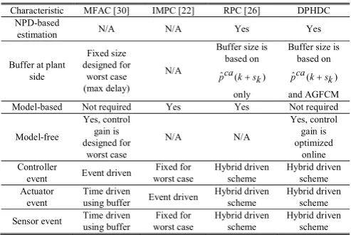
TABLEI
CHARACTERISTICS OF THE COMPARATIVE CONTROLLERS
Characteristic MFAC [30] IMPC [22] RPC [26] DPHDC
NPD-based
estimation N/A N/A Yes Yes
Buffer at plant side
Fixed size designed for
worst case (max delay)
N/A
Buffer size is based on
ˆca( )
p k sk
only
Buffer size is based on
ˆca( )
p k sk
and AGFCM
Model-based Not required Yes Yes Not required
Model-free
Yes, control gain is designed for
worst case
N/A N/A
Yes, control gain is optimized
online Controller
event Event driven
Fixed for worst case
Hybrid driven scheme
Hybrid driven scheme Actuator
event
Time driven
using buffer Event driven
Hybrid driven scheme
Hybrid driven scheme
Sensor event Time driven
using buffer
Fixed for worst case
Hybrid driven scheme
Hybrid driven scheme
Here, the robust predictive control (RPC) [26], the improved model predictive control (IMPC) [22], the typical MFAC with fixed weight factor[30] combined with a fixed buffer (tagged as MFAC), and the proposed DPHDC. The characteristics of these controllers are summarized in Table I. Configuration of the system is presented in Fig. 3 and clearly described in [25], [26]. The system plant can be expressed as
1
x k Ax k Bu k d k
y k Cx k
with d(k) is the unknown time-variant disturbance; and 235870 4934200 1 0
, , .
1 0 0 32298000
T
A B C
To tackle the tracking control with computation delays and disturbances, these were added to the system during the experiments. The computation delays were simulated using the real machine computation delays in [25] while two disturbance sources [26] were invoked. The first source was the time-variant magnetic load applied to the motor shaft while the second source was added to the feedback speed as:
( ) Rand ( )N Nsin(2 N ) 1
here AN was given randomly from 0.5 to 1; fN was varied from
1 to 5 Hz; RandN was a noise with power 0.005.
For the control comparison, the real-time network problems were detected and recorded through an experiment with a selected controller. This problem source was then re-used to generate the same working conditions for the other controllers.
B. Setting of Controller Parameters
Using Definition 1, the delay thresholds were selected as: 0.025 ,
com
s
t ca 0.035 and sc 0.035
s s
t t . The RPC and IMPC were constructed based on the linearized system model. The state feedback and integral control gains of the RPC were derived for the set of the total delay regions ranging from 0 to 0.095 with interval of 0.01s [31]. Meanwhile, its observer gain was derived as [1; 1.3217]. For the IMPC, based on its design [22], the sampling rate was selected as 0.1s to cover the total delay. The prediction horizon P and control horizon M were in turn selected in this case as 5 and 3, their corresponding weighting matrices was chosen as, Q = diag(0.4, 0, 0, 1) and R
= diag(0.01,0.01,0.01). The MFAC and DPHDC could be constructed without using the linearized plant model. For the MFAC, the buffer size was fixed as 5. As described in Section II and [30], the control parameters were set as
ˆ ˆ
1, 1, 1, (0) (0) 2,
10 ,5 and the weight
factor was set to20.5 corresponding to the worst network state. For the DPHDC, the control parameters were set as
5ˆ
1, 1, 1, (0) 2, 10 , 0 6.5, 1, s 10
.
C. Experiments and Discussions
The real-time speed tracking control experiments in the imperfect conditions have been then carried out using the comparative controllers. Here, the first disturbance source always applied to the motor shaft while the second disturbance source was only added to the feedback speed after 15 seconds.
The first experiment series were done to track a constant speed at 10rad/s. The results were then obtained in Fig. 4. During the first 15 seconds with small perturbations, both the controllers could drive the motor speed to follow the desired level well (steady-state-error (SSE) within 2%). With the MFAC, once packet dropouts in the backward channel were detected, the system response could be ideally estimated using (2) and the iteration algorithm. Thus, the vector of five-step-ahead control inputs was always generated and sent to the buffer to drive the motor. However, the MFAC could only ensure the system converge to the disturbed speed level around the desired set point because of lacking disturbance compensation.
0 5 10 15 20 25 30
0.00 0.02 0.04 0.00 0.01 0.02 0.03
Computation Delay; Estimated Delay
D
el
ay
[
s]
0.00 0.02
0.04 Network - Forward Delay (C-A); Estimated Delay
D
e
la
y
[s
]
PC Time [s]
Network - Feeback Delay (S-C); Estimated Delay
D
el
ay
[
s]
0
1 Packet Dropouts; Estimated Packet Dropouts
P
ac
ke
t D
ro
p
ou
ts 0 2 4 6
O
S
B
Fig. 5. Step tracking: one-step-ahead prediction of the delays and forward packet dropouts and OSB size of the DPHDC.
0 5 10
S
p
ee
d
[r
a
d/
s]
Reference Speed; RPC;
IMPC; MFAC; DPHDC
0 5 10 15 20 25 30
-0.4 0.0 0.4
RPC; IMPC;
MFAC; DPHDC
E
rr
o
r
[r
ad
/s
]
PC Time [s]
[image:9.595.86.506.374.741.2]Added 2nd disturbance souce at T=15s
Furthermore, due to use of fixed buffer size and fix weight factor, this controller could not adapt quickly to the system changes. Therefore once the disturbance level increased during the last 15 seconds, the tracking performance significantly deteriorated. With the IMPC, the system adaptation was slower than the others because the fixed large sampling period was used to cover the total system delays. Nevertheless, the steady response over the test was better than that of the MFAC due to the integration of speed tracking error minimization in conducting the optimal control signal. The most precise performances were achieved by the last two control options. This came as no surprise because these controllers possess the unique characteristics of the grey models, adaptive buffers, hybrid driven mechanism and adaptive control gains based on the network problem detection and disturbance rejection mechanisms. Due to the same use of prediction technique, the one-step-ahead delay prediction with high accuracy could be observed by either the RPC or the DPHDC scheme as plotted in sub-plots 1 to 4 from bottom of Fig. 5. The packet dropouts’ plot shows the detection/estimation results on both the channels) while the OSB size of the DPHDC was observed as plotted in the top sub-plot of Fig. 5. The tracking results of these two methods were almost similar. Nonetheless in the RPC, the buffer with the tight selection of buffer size based on the package dropout prediction only could lead to small delays and even small increases of SSE in system response if the network problem was not properly estimated. This could be clearly demonstrated through Fig. 6. Here, the RPC was tested in which a random faulty signal was added to the network problem estimation of this controller. The tracking result was then
compared against the performances of the RPC and DPHDC. In addition, the RPC required the system knowledge well represented in the form of linearized model and the observer gains needed to be off-line calculated to cover the delay range. These could hinder the applicability of this method. On the contrary, the DPHDC is capable of producing the robust control actions without the system knowledge. With the proposed DPHDC, the buffer size was optimally adjusted based on both the prediction and tracking performances and the network status. Thus, the continuous optimal control inputs to drive the motor could be ensured. The tracking performances using the compared controllers were then summarized in Table II.
Next, to confirm the capability of the proposed approach over the other ones, the second experiment series were done for a multi-step speed tracking control profile under the same perturbed environment. The tracking results were obtained as plotted in Fig. 7. Similar to the first test, the slowest adaptation was observed by the IMPC while the lowest stability was obtained by the MFAC. In some regions, the IMPC and MFAC tracking results were quite similar as they were both designed for the worst network conditions (Table I) and, therefore, the system adaptation was slowly achieved. The RPC and DPHDC showed their superiority performances over the IMPC and MFAC. As numerically shown in Table II, although the RPC could bring to the smallest SSE and mean square error, the smooth response and quick adaptation were only guaranteed by the DPHDC. Both of these characteristics and the high applicability make the proposed control scheme to be the best solution for the considered NCS.
0 5 10 15 20 25 30
0 5 10 15 20
Added 2nd disturbance souce at T=15s
S
pe
e
d
[
ra
d
/s
]
PC Time [s] Reference Speed
RPC IMPC MFAC DPHDC
Fig. 7. Multi-step tracking: performance comparison.
5 10
S
p
e
ed
[
ra
d
/s
]
Reference Speed; RPC;
Faulty RPC; DPHDC;
0 5 10 15 20 25 30
-0.4 0.0 0.4
RPC; Faulty RPC; DPHDC
E
rr
o
r
[r
a
d/
s]
PC Time [s]
[image:10.595.84.507.84.381.2]Added 2nd disturbance souce at T=15s
TABLEII
COMPARISON OF NCSPERFORMANCES USING DIFFERENT CONTROLLERS
Controller
Step responses Percent of
Overshoot [%] Time [s] Settling SSE [%] [15~30s] [rad/s]Mean Square Error 210-2 15~30s]
RPC 0.47 1.74 1.63 1.14
IMPC 0.25 1.53 3.56 6.48
MFAC 0.38 1.36 8.44 21.88
DPHDC 0.39 0.61 1.87 1.83
VIII. CONCLUSIONS
In this paper, the data-based predictive hybrid driven control approach has been successfully introduced for a class of NCSs under random delays, packet dropouts and disturbances. The combination of the advanced modules, including the PIAGM(1,1), the hybrid driven mechanism, the AGFCM-based OSB buffer and the PMFAC, could compensate well all the system issues without requiring the plant model. The robust tracking performance is theoretically proved and guaranteed by tuning online the control inputs via the weight factor and buffer size regulation. The applicability and capability of the proposed DPHDC have been validated through real-time experiments on the networked servomotor system with difference control methods.
APPENDIX A
As Remark 4, for an object with a data sequence
1 , 2 ,...,
obj obj O obj O obj Om
Y y t y t y t , the raw input grey sequence Yraw is derived as (8). From (8), define
1; 2,..,
Ok Ok Ok
t t t k m
, the following two cases are considered:
Case 1 – the object has equal time-interval signal, or unequal time-interval signal satisfying a time sequence checking in (A1), each data point of Yraw is obtained as (A2)
1
1.1; ; 2,...,
Ok
Ok Ok O k
t
t t t k m
T
(A1)
here T is the desired sample time.
0
; 0 1; 1,..., ; .raw i obj Oi i
y t y t i n n m (A2)
Case 2 – the object having unequal time-interval signal which does not satisfy (A1), each data point of Yraw is derived
using the SP algorithm A3( 0 0)
i
0
1 1 1
1 2 3
0
1 1
; ;
; 2,..., ; ; 1,..., 1 raw Object i i
raw i k k i Ok k i Ok k i Ok
Om Ok i O k
y t y t t t T
y t Sa Sb t t Sc t t Sd t t
t t
t t t i n n floor k m
T
(A3) where:
Sa Sb Sc Sdk, k, k, k
k1,...,m1
is a [4 x m-1] coefficient matrix of the spline function going through the object data set
t y1, obj
t1
,...,
t ym, obj
tm
.From [3], the coefficient matrix can be computed using the following S-procedure:
S-step 1: Obtain the first column of the coefficient matrix as
; 1,..., 1. k obj OkSa y t k m (A4)
S-step 2: Generate a vectors h in size [1 x m-1]
1 .k O k Ok
h h k t t (A5)
S-step 3: Generate a vectors g in size [1 x m-2]
2 1
1
1
3
3
; 1,..., 2.
k obj O i obj O k
k
obj O k obj Ok k
g g k y t y t
h
y t y t k m
h
(A6)
S-step 4: Perform a tri-diagonal matrix algorithm to calculate the third column of the coefficient matrix as
1
1 2
1 1 1
2 3
2 2 2
2 1 2 1 2
0
1 0 0 0 0
0 0
0 0
0 0
0 0 0 0 1 0 0
m m m m m
Sc
g Sc
va vb vc
g Sc
va vb vc
va vb vc Sc g
(A7)
herevak h vbk; k 2
hkhk1
;vck hk1;k1,...,m2. By solving (A7) based on Gaussian elimination, the vector
Sck is then easily obtained
Scm0
.S-step 5: Calculate the second and fourth column
1
2 1
3
obj O k obj Ok k k k
k
k
y t y t Sc Sc h
Sb
h
(A8)
1 .
3
k k
k
k
Sc Sc
Sd
h
(A9)
REFERENCES
[1] J. Qiu, S. Member, H. Gao, and S. X. Ding, “Recent Advances on Fuzzy-Model-Based Nonlinear Networked Control Systems : A Survey,” IEEE Trans. Ind. Electron., vol. 63, no. 2, pp. 1207–1217, 2016.
[2] C. Hua and X. P. Liu, “A New Coordinated Slave Torque Feedback Control Algorithm for Network-Based Teleoperation Systems,”
IEEE/ASME Trans. Mechatronics, vol. 18, no. 2, pp. 764–774, 2013. [3] D. Q. Truong, K. K. Ahn, and N. T. Trung, “Design of an advanced time
delay measurement and a smart adaptive unequal interval grey predictor for real-time nonlinear control systems,” IEEE Trans. Ind. Electron., vol. 60, no. 10, pp. 4574–4589, 2013.
[4] B. W. Zhang, M. S. Branicky, and S. M. Phillips, “Stability of networked control systems,” IEEE Control Syst., vol. 21, no. 1, pp. 84–99, 2001. [5] C. Huang, Y. Bai, and X. Liu, “H-Infinity State Feedback Control for a
Class of Networked Cascade Control Systems With Uncertain Delay,”
IEEE Trans. Ind. Informatics, vol. 6, no. 1, pp. 62–72, 2010.
[6] B. Yang, U. Tan, A. B. Mcmillan, R. Gullapalli, and J. P. Desai, “Design and Control of a 1-DOF MRI-Compatible Pneumatically Actuated Robot With Long Transmission Lines,” IEEE/ASME Trans. Mechatronics, vol. 16, no. 6, pp. 1040–1048, 2011.
[7] D. Tian, D. Yashiro, and K. Ohnishi, “Wireless Haptic Communication Under Varying Delay by Switching-Channel Bilateral Control With Energy Monitor,” IEEE/ASME Trans. Mechatronics, vol. 17, no. 3, pp. 488–498, 2012.
[8] F. Yang, Z. Wang, Y. S. Hung, and M. Gani, “H∞ control for networked control systems with random communication delays.pdf,” IEEE Trans. Automat. Contr., vol. 51, no. 3, pp. 511–518, 2006.
[9] C. Choi and W. Lee, “Analysis and Compensation of Time Delay Effects in Hardware-in-the-Loop Simulation for Automotive PMSM Drive System,” IEEE Trans. Ind. Electron., vol. 59, no. 9, pp. 3403–3410, 2012.
[10] K. Kim, M. Sung, and H. Jin, “Design and Implementation of a Delay-Guaranteed Motor Drive for Precision Motion Control,” IEEE Trans. Ind. Informatics, vol. 8, no. 2, pp. 351–365, 2012.
prediction-based variable-period sampling approach for networked control systems,” Appl. Math. Comput., vol. 185, pp. 976–988, 2007.
[12] C. Lai and P. Hsu, “Design the Remote Control System With the Time-Delay Estimator and the Adaptive Smith Predictor,” IEEE Trans. Ind. Informatics, vol. 6, no. 1, pp. 73–80, 2010.
[13] D. López-echeverría and M. E. Magaña, “Variable Sampling Approach to Mitigate Instability in Networked Control Systems with Delays,”
IEEE Trans. Neural Networks Learn. Syst., vol. 23, no. 1, pp. 119–126, 2012.
[14] R. Yang, G. Liu, P. Shi, C. Thomas, and M. V Basin, “Predictive Output Feedback Control for Networked Control Systems,” IEEE Trans. Ind. Electron., vol. 61, no. 1, pp. 512–520, 2014.
[15] T. Chai, L. Zhao, J. Qiu, F. Liu, and J. Fan, “Integrated Network-Based Model Predictive Control for Setpoints Compensation in Industrial Processes,” IEEE Trans. Ind. Informatics, vol. 9, no. 1, pp. 417–426, 2013.
[16] Z. Pang, G. Liu, D. Zhou, S. Member, and M. Chen, “Output Tracking Control for Networked Systems : A Model-Based Prediction Approach,”
IEEE Trans. Ind. Electron., vol. 61, no. 9, pp. 4867–4877, 2014. [17] P. Ignaciuk, “Nonlinear Inventory Control With Discrete Sliding Modes
in Systems With Uncertain Delay,” IEEE Trans. Ind. Informatics, vol. 10, no. 1, pp. 559–568, 2014.
[18] A. Baños, F. Perez, and J. Cervera, “Network-Based Reset Control Systems With Time-Varying Delays,” IEEE Trans. Ind. Informatics, vol. 10, no. 1, pp. 514–522, 2014.
[19] H. Gao, T. Chen, and J. Lam, “A new delay system approach to network-based control,” Automatica, vol. 44, pp. 39–52, 2007.
[20] H. Gao and T. Chen, “Network-Based H∞ Output Tracking Control,”
IEEE Trans. Automat. Contr., vol. 53, no. 3, pp. 655–667, 2008. [21] C. Peng and Q. L. Han, “On Designing a Novel Self-Triggered Sampling
Scheme for Networked Control Systems with Data Losses and Communication Delays,” IEEE Trans. Ind. Electron., vol. 63, no. 2, pp. 1239–1248, 2016.
[22] R. Lu, Y. Xu, and R. Zhang, “A New Design of Model Predictive Tracking Control for Networked Control System under Random Packet Loss and Uncertainties,” IEEE Trans. Ind. Electron., vol. PP, no. 99, pp. 6999–7007, 2016.
[23] L. Repele, R. Muradore, D. Quaglia, and P. Fiorini, “Improving Performance of Networked Control Systems by Using Adaptive Buffering,” IEEE Trans. Ind. Electron., vol. 61, no. 9, pp. 4847–4856, 2014.
[24] H. Li and Y. Shi, “Network-Based Predictive Control for Constrained Nonlinear Systems With Two-Channel Packet Dropouts,” IEEE Trans. Ind. Electron., vol. 61, no. 3, pp. 1574–1582, 2014.
[25] D. Q. Truong and K. K. Ahn, “Robust Variable Sampling Period Control for Networked Control Systems,” IEEE Trans. Ind. Electron., vol. 62, no. 9, pp. 5630–5643, 2015.
[26] D. Q. Truong, K. K. Ahn, and J. Marco, “A Novel Robust Predictive Control System Over Imperfect Networks,” IEEE Trans. Ind. Electron., vol. 64, no. 2, pp. 1751–1761, 2017.
[27] Z. Hou and Z. Wang, “From model-based control to data-driven control : Survey , classification and perspective,” Inf. Sci. (Ny)., vol. 235, pp. 3– 35, 2013.
[28] Z. Hou and X. Bu, “Model free adaptive control with data dropouts,”
Expert Syst. Appl., vol. 38, no. 8, pp. 10709–10717, 2011.
[29] X. Bu, F. Yu, Z. Hou, and H. Zhang, “Model-Free Adaptive Control Algorithm with Data Dropout Compensation,” Math. Probl. Eng., vol. 2012, pp. 1–14, 2012.
[30] Z. Pang, G. Liu, D. Zhou, and D. Sun, “Data-Based Predictive Control for Networked Nonlinear Systems With Network-Induced Delay and Packet Dropout,” IEEE Trans. Ind. Electron., vol. 63, no. 2, pp. 1249– 1257, 2016.
[31] N. Vatanski, J. P. Georges, C. Aubrun, E. Rondeau, and S. L. Jämsä-Jounela, “Networked control with delay measurement and estimation,”
Control Eng. Pract., vol. 17, no. 2, pp. 231–244, 2009.
[32] J. Jasperneite and K. Shehab, “Enhancements to the Time Synchronization Standard IEEE-1588 for a System of Cascaded Bridges,” in 5th IEEE Int. Workshop on Factory Communication Systems (WFCS’04), 2004, pp. 239–244.
[33] X. Chen, D. Li, S. Wang, H. Tang, and C. Liu, “Frequency-Tracking Clock Servo for Time Synchronization in Networked Motion Control Systems,” IEEE Access, vol. 5, pp. 11606–11614, 2017.
[34] D. Q. Truong and K. K. Ahn, “Force control for hydraulic load simulator using self-tuning grey predictor - fuzzy PID,” Mechatronics, vol. 19, no. 2, pp. 233–246, 2009.
[35] E. Kayacan, B. Ulutas, and O. Kaynak, “Grey system theory-based models in time series prediction,” Expert Syst. Appl., vol. 37, no. 2, pp. 1784–1789, 2010.
[36] J. G. Vanantwerp and R. D. Braatz, “A tutorial on linear and bilinear matrix inequalities,” J. Process Control, vol. 10, pp. 363–385, 2000. [37] E. I. Papageorgiou and P. P. Groumpos, “A new hybrid method using
evolutionary algorithms to train Fuzzy Cognitive Maps,” Appl. Soft Comput., vol. 5, no. 4, pp. 409–431, 2005.
[38] J. L. Salmeron, “Modelling grey uncertainty with fuzzy grey cognitive maps,” Expert Syst. Appl., vol. 37, no. 12, pp. 7581–7588, 2010.
Truong Quang Dinh (M’18) received the B.S
degree in the department of Mechanical Engineering from Hochiminh City University of Technology, Hochiminh, Vietnam, in 2001, and the Ph.D. degree in the School of Mechanical Engineering from University of Ulsan, Ulsan, Korea, in 2010.
He is currently an Assistant Professor at Warwick Manufacturing Group (WMG), University of Warwick, Coventry, UK. His research interests focus on control theories and applications, fluid power control systems, energy saving and power management systems, low carbon technologies for transports and construction sectors, and smart sensors and actuators. He is a Member of IEEE, and IES.
James Marco received the Eng.D. degree from
the University of Warwick.
He is currently an Associate Professor at the Warwick Manufacturing Group (WMG), University of Warwick, Coventry, UK. His research interests include systems engineering, real-time control, systems modelling, design optimisation, design of energy management control systems. In particular, these generic and enabling technologies relate to the design of new low carbon technologies for the transport and energy storage sectors.
Dave Greenwood received M.A. degree from the
University of Cambridge, UK, in 1993, the M.Sc. degree from Chalmers University of Technology, Sweden, in 2008.
He joined WMG as a Professor in 2014 from Ricardo UK Ltd. He currently leads the Advanced Propulsion Systems team at Warwick Manufacturing Group (WMG), University of Warwick, Coventry, UK. His research interests include vehicle powertrain, energy storage, energy conversion and management. He is a Board Member at the Low Carbon Vehicle Partnership (LowCVP) and a member of the Automotive Council Technology Group. He is also a Member of the EPSRC’s Energy Scientific Advisory Committee and the Advanced Propulsion Centre (APC) Advisory Board.
Kyoung Kwan Ahn (M’02) received the B.S.
degree in the department of Mechanical Engineering from Seoul National University in 1990, the M.Sc. degree in Mechanical Engineering from Korea Advanced Institute of Science and Technology (KAIST) in 1992 and the Ph.D. degree with the title “A study on the automation of out-door tasks using 2 link electro-hydraulic manipulator from Tokyo Institute of Technology in 1999, respectively.
Jong Il Yoon received the Ph.D. from the University of Ulsan, Ulsan, Korea, in 2014.