econ
stor
www.econstor.eu
Der Open-Access-Publikationsserver der ZBW – Leibniz-Informationszentrum Wirtschaft
The Open Access Publication Server of the ZBW – Leibniz Information Centre for Economics
Standard-Nutzungsbedingungen:
Die Dokumente auf EconStor dürfen zu eigenen wissenschaftlichen Zwecken und zum Privatgebrauch gespeichert und kopiert werden. Sie dürfen die Dokumente nicht für öffentliche oder kommerzielle Zwecke vervielfältigen, öffentlich ausstellen, öffentlich zugänglich machen, vertreiben oder anderweitig nutzen.
Sofern die Verfasser die Dokumente unter Open-Content-Lizenzen (insbesondere CC-Lizenzen) zur Verfügung gestellt haben sollten, gelten abweichend von diesen Nutzungsbedingungen die in der dort genannten Lizenz gewährten Nutzungsrechte.
Terms of use:
Documents in EconStor may be saved and copied for your personal and scholarly purposes.
You are not to copy documents for public or commercial purposes, to exhibit the documents publicly, to make them publicly available on the internet, or to distribute or otherwise use the documents in public.
If the documents have been made available under an Open Content Licence (especially Creative Commons Licences), you may exercise further usage rights as specified in the indicated licence.
zbw
Leibniz-Informationszentrum WirtschaftBriglevics, Tamás; Schuh, Scott
Working Paper
U.S. consumers´ demand for cash in the era of low
interest rates and electronic payments
Working Papers, Federal Reserve Bank of Boston, No. 13-23 Provided in Cooperation with:
Federal Reserve Bank of Boston
Suggested Citation: Briglevics, Tamás; Schuh, Scott (2013) : U.S. consumers´ demand for cash in the era of low interest rates and electronic payments, Working Papers, Federal Reserve Bank of Boston, No. 13-23
This Version is available at: http://hdl.handle.net/10419/107218
No. 13-
23
U.S. Consumer Demand for Cash in the Era
of Low Interest Rates and Electronic
Payments
Tamás Briglevics and Scott Schuh
Abstract:
U.S. consumers’ demand for cash is estimated with new panel micro data for 2008‒2010 using econometric methodology similar to Mulligan and Sala-i-Martin (2000); Attanasio, Guiso, and Jappelli (2002); and Lippi and Secchi (2009). We extend the Baumol-Tobin model to allow for credit card payments and revolving debt, as in Sastry (1970). With interest rates near zero, cash demand by consumers using credit cards for convenience (without revolving debt) has the same small, negative, interest elasticity as estimated in earlier periods and with broader money measures. However, cash demand by consumers using credit cards to borrow (with revolving debt) is interest inelastic. These findings may have aggregate implications for the welfare cost of inflation because the nontrivial share of consumers who revolve credit card
debt are less likely to switch from cash to credit. In the 21st century, consumers get cash from
bank and nonbank sources with heterogeneous transactions costs, so withdrawal location is essential to identify cash demand properly.
Keywords:
cash demand, Baumol-Tobin model, Survey of Consumer Payment Choice,
SCPC
JEL Classifications:
E41, E42
Tamás Briglevics is a research associate in the Center for Consumer Payments Research in the research department of the Federal Reserve Bank of Boston and a graduate student at Boston College. Scott Schuh is a senior economist and policy advisor and the director of the Center for Consumer Payments Research in the research department of the Federal Reserve Bank of Boston. Their e-mail addresses are [email protected] and [email protected], respectively.
This paper, which may be revised, is available on the web site of the Federal Reserve Bank of Boston at http://www.bostonfed.org/economic/wp/index.htm.
We thank Susanto Basu, Christopher Baum, Marieke Bos, John Driscoll, Chris Foote, Simon Gilchrist, Peter Ireland, Arthur, Lewbel, Chester Spatt, Ellis Tallman, Bob Triest, and seminar participants at the Boston Fed, Boston College, Boston University, System Committee on Business and Financial Analysis 2011 at the Cleveland Fed, the Annual Meeting of the Hungarian Economic Society 2011, the Midwest Finance Association’s Annual Meeting 2012, and the Deutsche Bundesbank’s Conference on the Usage, Costs and Benefits of Cash for helpful comments and discussion. All remaining errors are ours.
The views expressed in this paper are those of the authorand do not necessarily represent the views of the Federal Reserve Bank of Boston or the Federal Reserve System.
1
Introduction
Reports of the demise of cash as a means of payment in the U.S. economy may be pre-mature. The new Survey of Consumer Payment Choice (SCPC) indicates that demand for cash by U.S. consumers declined significantly during the past quarter century, as shown in
Table1. The average stock of cash carried for transactions fell more than 30 percent in real
terms since the mid-1980s (from $112 to $79) and the typical amount of a cash withdrawal fell nearly 50 percent (from $261 to $132). However, the number of withdrawals actually increased and cash still accounts for more than one in four payments made by consumers.
So, cash is not “dead”—at least not yet.1
New evidence on cash management comes at a potentially enlightening time to re-evaluate money demand. During the financial crisis of 2007–2009, short-term interest rates dropped to near zero, so the opportunity cost of holding M1 in currency, rather than in interest-bearing deposit accounts, essentially vanished. At the same time, consumer cash withdrawals increased and cash payments by consumers surged, according to Foster et al. (2011), even as the economy recovered. Furthermore, during the quarter century leading up to this unique period, the U.S. payment system experienced a transformation from paper instruments (cash and checks) to a wide range of payment cards and other electronic means of authorizing, clearing, and settling payments. Some technological developments affected the transactions costs of acquiring and managing cash as well.
This paper estimates consumer demand for cash in an era of low interest and
elec-tronic payments.2 Our econometric methodology follows recent attempts to estimate
var-ious forms of money demand using cross-sectional micro data for U.S. households, as in Mulligan and Sala-i-Martin (2000), and time-series panel micro data for Italian households, as in Attanasio, Guiso, and Jappelli (2002) and especially Lippi and Secchi (2009), to which our study is closest. Naturally, our econometric specification is shaped by data availabil-ity, but the model is quite similar to recent studies, with relatively minor differences in data sources and control variables. Our contribution meets the challenge of Ireland (2009): “Finding additional sources of information about the limiting behavior of money demand as interest rates approach zero, whether from time series data from other economies or from cross-sectional data as suggested by Casey B. Mulligan and Xavier Sala-i-Martin (2000), remains a critical task for sharpening existing estimates of the welfare cost of modest rates of inflation”[page 1049].
Our econometric model also extends the literature in two ways. First, it incorporates a reduced-form test of the theoretical conjecture advanced by Sastry (1970) that credit card revolving debt should influence consumer demand for money. Following the literature, es-timation is based on an applied version of the Baumol (1952)–Tobin (1956) (BT henceforth)
1Evans et al. (2013) draws a similar conclusion.
2Unfortunately, the scope of investigation is limited to cash rather than M1 because analogous data on consumer deposit accounts are not available at this time.
1984/86 2008-10
Average Average Change
Value of cash in pocket, purse or wallet
Average amount ($) 112 79 -33
(share of monthly median income (%)) (2.9) (1.9) (1.0)
Number of withdrawals per month (#) 4.3 5.6 1.3
Usual amount per withdrawal ($) 261 132 -129
Value of cash withdrawals
estimated monthly amount∗($) 817 488 -329
(share of monthly median income (%)) (21.0) (12.0) (-9.0)
Number of cash payments
per month (#) na 19.2 na
share in number of all transactions (%) na 27.0 na
All numbers are 2010 dollar values unless noted otherwise.
Sources:SCTAU for 1984-86, SCPC for 2008-10, median incomes from Census Bureau.
∗Derived from typical number of withdrawals and typical amount of withdrawal at the
level of individual respondents. May not equal actual total withdrawals.
Table 1: U.S. consumers’ cash management
model. However, our econometric model separately identifies the interest elasticity of cash demand for credit card “convenience users” (those who pay their credit bill in full each month) and credit card “revolvers” (consumers who carry some credit card debt across months). Revolving debt in the United States has surged in importance since the mid-1980s, reaching $1 trillion (a tenfold nominal increase) and 9 percent of disposable income (a
three-fold increase) by the time of the financial crisis.3 Second, our econometric model controls
for consumer payment choices (adoption and use of payment instruments) and cash man-agement practices (withdrawals) that reflect technological changes and the transformation from paper to electronic means of payment.
One key result is that the interest elasticity of cash demand depends directly on whether consumers carry revolving debt, and hence indirectly on the interest rate for credit card debt. Convenience users of credit cards exhibit essentially the same small, negative interest elasticity in 2008–2010 as were estimated in earlier periods and with broader money mea-sures (see, for example, Ireland (2009)). In contrast, cash demand by credit card revolvers is interest inelastic. The underlying intuition of this result is simple. Convenience users take advantage of the interest-free grace period by settling more of their transactions via credit to reduce forgone interest income on cash holdings. But substitution from cash to credit is costly for revolvers, who accrue interest charges immediately after swiping their credit cards, so their cash demand may not respond when the opportunity cost rises.
Another key result is that technological factors, which likely reflect transactions costs of acquiring and managing cash, have a significant impact on consumer demand for cash in the 21st century. Although we control for primary cash withdrawal location, as in previous studies such as Lippi and Secchi (2009), Amromin and Chakravorti (2009), and Carbó-Valverde and Rodrìguez-Fernandéz (2009), we do not find evidence that bank density or
ATM diffusion affects U.S. consumer demand for cash conditional on primary location.4
However, some U.S. consumers now withdraw cash from nonbank sources, such as retail stores (cash back from a debit card purchase), financial stores (for example, check cashing), employers, and family members. These nonbank alternatives may supply cash at different transactions costs, which may influence the amount and frequency of cash withdrawals and holdings. We find that controlling for the consumer’s source of cash in estimation is crucial to identifying money demand properly.
Together, these findings may have aggregate implications for the welfare cost of infla-tion. Because revolvers’ cash demand is interest inelastic, their demand curve is vertical and they are unlikely to reduce their cash holdings when inflation and short-term interest rates rise. Revolvers also are less likely to reap the full gains from financial innovations that reduce the transactions costs of getting cash because they rely relatively more on cash. And revolvers respond less to increases in the interest rate on short-term liquid accounts because that rate is significantly below the rate on credit card debt. According to the SCPC, a nontrivial share of consumers report having revolving credit card debt (29.5 percent in 2010) and these revolvers hold a nontrivial share (25.2 percent) of the stock of cash held by consumers.
The remainder of the paper is organized as follows. Section 2 provides a brief review
of the most relevant literature. Section3contains a description of the new data used in the
paper. Section4 reviews the theory behind microeconometric studies of money demand.
Section5 explains our econometric approach used to derive the results described in
Sec-tion6. Section7discusses the implications of our key result for the welfare cost of inflation
literature, while Section8concludes.
2
Literature Review
The literature on money demand is vast and a full survey is beyond the scope of this paper. Here, we briefly summarize the studies most relevant to this paper, mainly those based on micro data estimation. For more comprehensive surveys of the money demand literature, see Barnett, Fisher, and Serletis (1992) and Duca and VanHoose (2004).
From a macroeconomic perspective, the interest elasticity estimates at near-zero interest
4This negative result may also be due to the fact that the diffusion of ATM technology in the United States was essentially complete by 2008–2010, and the U.S. market has many banks with a pervasive branch and ATM system.
rates are of crucial importance for accurate computations of the welfare cost of inflation using Bailey (1956)’s method. This issue is at the core of the debate illustrated by Robert E. Lucas (2000) and Ireland (2009), both of which used aggregate data on M1 (cash plus demand deposits) to estimate money demand. While our estimates are derived from only
a portion of the economy’s total money demand,consumers’demand for cash, our interest
elasticity estimates are quite similar to the small negative elasticities found in macro studies covering earlier time periods and broader measures of money.
An alternative approach to estimating money demand is to use micro data from house-hold and consumer surveys. Most such studies also are based on BT models of consumers’ demand for some component of money and from periods with higher interest rates, and it is unclear whether they would generalize well to a low interest rate environment. The latest cash demand study for the U.S. appears to be Daniels and Murphy (1994), which used the Survey of Currency and Transaction Account Usage (SCTAU) from 1984 and 1986. The authors estimated a very small, positive interest elasticity of cash demand and noted that credit cards may explain this finding, as in the theoretical model of Lewis (1974), but could not test their conjecture because the SCTAU does not contain credit card data. Us-ing the 1989 wave of the Survey of Consumer Finance (SCF), Mulligan and Sala-i-Martin (2000) estimated U.S. households’ demand for balances in demand deposit accounts and emphasized the importance of the decision to adopt interest-bearing accounts (extensive margin) for aggregate interest elasticity. However, due to a lack of interest rate data, their estimate of the interest elasticity of interest-bearing account holders (intensive margin) was imprecise.
Other recent studies of cash demand used micro data from European countries: At-tanasio, Guiso, and Jappelli (2002), Lippi and Secchi (2009), and Alvarez and Lippi (2009) for Italy, Carbó-Valverde and Rodrìguez-Fernandéz (2009) for Spain, Stix (2004) for Austria, and Bounie and Francois (2008) for France. Our paper is closest to the methodology and ex-position in Lippi and Secchi (2009), which refined the cash demand estimates of Attanasio, Guiso, and Jappelli (2002) by estimating a tractable, partial equilibrium model of the effects of improvements in transactions technologies on cash demand. While we find significant level effects of different account access technologies (for example, ATM users withdraw less cash than those who use bank tellers), we do not find different interest elasticities by the diffusion of technology. Alvarez and Lippi (2009) looks at the effect of technological change in a model where cash spending is stochastic and confirms the finding of Lippi and Secchi (2009) about the effects of technological change. In the structural model of Alvarez and Lippi (2009), the interest elasticity converges to zero as the interest rate goes to zero, in line with our findings.
A few other studies have considered the link between credit cards and liquid assets. Looking at the effect of credit card use on money demand, White (1976) found that credit
card users reduce the balance of their checking account by roughly the amount of credit card spending and Duca and Whitesell (1995) found similar effects. However, neither of these two studies estimated the interest elasticity of money demand.
Substitution from cash to credit by households has been introduced in a number of models as a way to avoid the inflation tax at the social cost of costly credit provision (see Cooley and Hansen (1991), Gillman (1993), Dotsey and Ireland (1996), and Khan, King, and Wolman (2003)). However, to our knowledge, the empirical finding that credit card users who face different borrowing rates appear to use this channel differently is novel. Telyukova (2013) and Telyukova and Visschers (forthcoming) use the Lagos and Wright (2005) framework to analyze precautionary demand for liquid assets and its effects on the welfare cost of inflation. These papers also use micro data to calibrate the key parameters governing the choice between “cash” (which in their case includes checks and debit) and credit goods, but their focus is on the effects of idiosyncratic liquidity shocks. In particular, they assume that credit and money are perfect substitutes in the markets where credit is available. Our results show that this assumption may not be an accurate description of consumers who revolve credit card debt. Silva (2012) revisited the welfare cost of infla-tion estimates based on cash in advance models and showed that incorporating multiple withdrawals over a period increases the welfare cost estimates substantially, but he did not consider the choice between credit cards and cash.
3
Data and Empirical Evidence
This section describes the data sources used in this study, presents descriptive statistics,
and discusses the key features of the data. See Appendix B for more detailed variable
definitions.
3.1 Data Sources
The primary data source is the 2008–2010 SCPC, which contains comprehensive information on consumer adoption and use of all common U.S. payment instruments, including cash management practices. Each annual survey is administered to members of the American Life Panel, a representative sample of U.S. adults (18+) originally developed by the RAND Corporation. The reporting unit is a consumer, rather than a household, although some household characteristics are included. The SCPC samples contain about 1,000 respondents in 2008 and 2,000 in 2009–2010, with a significant longitudinal component. Roughly 85 to 90 percent of respondents return each year, so the pooled time-series cross-section of SCPC data also forms an unbalanced panel with 715 panelists in all three years and about 1,900
in 2009–2010.5
The SCPC collects data on consumer cash holdings and cash withdrawals. For holdings, consumers are asked how much cash they have in: 1) their pocket, purse, or wallet (referred to as “cash in wallet”); and 2) their house, car, or other property (“cash on property”). Total
cash holdings is the sum of these two measures.6 The SCPC measures of cash holdings may
differ from balances consumers hold for actual cash transactions. Cash on property likely includes holdings for speculative or other nontransactional purposes, but may also include storage of some cash intended for transactions, so cash in wallet may understate actual cash
balances held for transactions.7 However, the relatively objective, tangible classification of
cash holdings by physical location may be easier for respondents to answer accurately. For cash withdrawals, consumers are asked two questions: 1) the amount of cash they withdraw most often (the modal amount); and 2) the number of withdrawals they make in a typical month. Consumers are also asked each of these questions for two withdrawal loca-tions: 1) the location from which they withdraw cash most often (primary); and 2) all other locations. The withdrawal amount question reduces the mental burden on respondents to calculate averages of potentially diverse cash withdrawals. Consequently, the actual mean withdrawal could differ significantly from the reported modal withdrawal. Nevertheless, total cash withdrawals per month is approximated by adding the products of the modal withdrawal and the average number of withdrawals for the primary location and all other locations.
To summarize, the SCPC cash measures are close, but not identical, to the concepts used in basic theoretical models of cash demand. However, the usual (modal) amount of cash withdrawal may be a better analogue to the cash withdrawal variable in the BT model than actual withdrawals because the latter could be influenced by random events not captured by
the basic BT model.8 Similarly, the usual number of withdrawals at the favorite location fits
well with the theoretical concept, although it may be harder to accurately recall the usual frequency of withdrawals than the usual amount withdrawn. Therefore, the regression analysis focuses on the amount of cash usually withdrawn, the number of withdrawals, and the cash in wallet measures, since these seem to be most closely related to transactions balances.
6Because these questions do not require respondents to recall past behavior, cash holdings may be a more accurate measure of cash activity. However, little is known about consumers’ willingness to report cash hold-ings accurately, especially cash held for illegal purposes. Nevertheless, response rates are very high and the largest reported values are tens of thousands of dollars.
7The SCPC measures of cash management are slightly different from those in Attanasio, Guiso, and Jappelli (2002) and Lippi and Secchi (2009), which are based on the Survey of Household Income and Wealth (SHIW) collected by the Bank of Italy. The SHIW measures the amount of cash holdings a household usually keeps for everyday expenses, which in theory corresponds better to the BT theory. However, these types of responses depend on the (in)ability of respondents to accurately report their subjective, intended transactions balances. In contrast, the SCPC relies on a less subjective measure of cash holdings by a physical location (wallet or property) at the time of the survey. Each approach likely contains some measurement error.
8For models with stochastic cash-flows, see Miller and Orr (1966), Bar-Ilan (1990), Bar-Ilan, Perry, and Stadje (2004) and Alvarez and Lippi (2013).
SCPC 2008
SCPC 2009
SCPC 2010
0 .2 .4 .6 Interest yield (%) 0 50 100 150 Dollars ($) Sep 08 Sep 08 Dec 08 Sep 08 Dec 08 Mar 09 Sep 08 Dec 08 Mar 09 Jun 09 Sep 08 Dec 08 Mar 09 Jun 09 Sep 09 Sep 08 Dec 08 Mar 09 Jun 09 Sep 09 Dec 09 Sep 08 Dec 08 Mar 09 Jun 09 Sep 09 Dec 09 Mar 10 Sep 08 Dec 08 Mar 09 Jun 09 Sep 09 Dec 09 Mar 10 Jun 10 Sep 08 Dec 08 Mar 09 Jun 09 Sep 09 Dec 09 Mar 10 Jun 10 Sep 10 Sep 08 Dec 08 Mar 09 Jun 09 Sep 09 Dec 09 Mar 10 Jun 10 Sep 10 Dec 10 Sep 08 Dec 08 Mar 09 Jun 09 Sep 09 Dec 09 Mar 10 Jun 10 Sep 10 Dec 10 Mar 11Checking account yield (right scale) Money market yield (right scale) Average cash withdrawal (left scale)
Figure 1: Cash withdrawals and interest rates over the sample period
The SCPC also contains data on the types of bank accounts held by consumers (checking and saving), the institutions in which they hold their primary accounts, and the interest rate on their primary checking accounts. However, the SCPC does not contain data on the dollar amounts held in bank accounts or all of the crucial information needed on the opportunity cost of holding cash — in particular, the interest rates on money-market and other savings accounts. For the latter, we turn to a second data source, the Bank Rate Monitor (BRM)
dataset (see Section3.3for details), which has these interest rate data at the state level and is
merged with the SCPC. In addition to providing data from both before and during the low-interest environment, an important advantage of using the SCPC longitudinal panel micro data to estimate cash demand is that the dataset gives researchers the ability to identify interest elasticity by leveraging the time-varying cross-sectional heterogeneity in consumer bank accounts and interest rates, which is unavailable from aggregate times series data.
Figure 1 illustrates our sample period and foreshadows the basic results of the paper.
It plots the usual amount of cash withdrawn per consumer from his or her primary loca-tion (bars) along with the average yields for interest–bearing checking and money-market accounts for 2008–2011. Short-term interest rates declined notably from the period of the 2008 SCPC to the period of the 2009 SCPC, which was conducted slightly later in the fall than in 2008 and 2010. Consistent with the basic theories of money demand, the decrease in yields was mirrored by an increase in cash withdrawals over our sample period. Foster et al. (2011) report that the cash share of monthly consumer payments also increased 7.4 percentage points from 2008 to 2009.
Admittedly, this highly unusual period of financial crisis and recovery may hold al-ternative explanations for why consumer cash management practices changed, such as increased attention to budgeting. However, analyzing individual-level data provides the flexibility and potential benefit of controlling for a number of these alternative explana-tions. For example, our analysis can be restricted to the subsample of credit card adopters so that account closures do not influence the results.
As an example of the need to control for micro heterogeneity, the SCPC provides strik-ing evidence that cash management is affected by the location from which consumers
ob-tain their cash. Figure 2 displays the average amounts of cash withdrawn from seven
locations—ATM, bank teller, check cashing store, cash back from a debit card purchase (at a retail store), employer, family, and other—and the shares of consumers who most often withdraw cash from that location. The average amount of cash withdrawal varies widely, from less than $50 for cash back to about $300 at a check cashing store. Not surprisingly, most consumers (about four-fifths) get cash most often from an ATM or bank teller. But even among these most common locations the amount withdrawn varies significantly, as amounts withdrawn from bank tellers are almost twice as much as withdrawals from an ATM. Very large amounts are also withdrawn from employers and other locations, although relatively few consumers get their cash from these locations.
0 .1 .2 .3 .4 .5 Share of consumers 50 100 150 200 250 300 Dollars ($)
ATM Bank teller Check casher Cashback Employer Family Other
Average withdrawal amount (left scale)
Share of consumers using as primary location (right scale)
Figure 2: Cash withdrawals by location
The types of withdrawal locations, and the variation in withdrawal amounts across them, suggest diversity in transaction costs across locations of cash withdrawals for con-sumers. Econometrically, accounting for this withdrawal heterogeneity is important for
fitting the cash withdrawal data well. It also serves as an approximate individual fixed effect, which cannot be included in the econometric model due to an insufficient number of time-series observations per consumer, by representing the mean withdrawal of consumers grouped by primary location.
3.2 Descriptive statistics
Table 2 reports descriptive statistics for the key variables for the entire SCPC sample
(first three columns) and the econometric estimation subsample (remaining three columns), which comprises only consumers who had adopted a credit card and interest-bearing bank
account (100 percent adoption rates in both cases). Section4.1describes the motivation and
methodology of the sample selection in more detail.
Consumers withdraw more than $100 in a typical transaction and keep a little more than half of this amount in their wallet on average. The relationship between cash in wallet and on property is particularly interesting. While average cash holdings on property are up to four times higher than cash in wallet, the median of the cash on property variable is only half the size of median cash holdings in wallet. For the cash variables in general, average values are much higher than the median values and the standard errors are quite large, especially in 2010. Together, these facts reflect the existence of a relatively small proportion of consumers who hold and withdraw very large amounts of cash. The number of cash withdrawals ranges from 4.3 to 5.7 per month.
Adoption rates are very high for checking accounts (91 percent or more) and any interest–bearing account (82 percent or more). The adoption of savings accounts decreases about 7 percentage points from 2008 to 2009, most likely due to a change in the survey questionnaire, and then stays flat. More importantly, only 15 to 20 percent of the
respon-dents do not have some type of interest–bearing accounts in the three sample years.9 About
85 percent of consumers have an ATM or debit card. Credit card adoption by consumers was 78.3 percent in 2008 but dropped to 71.2 percent by 2010. About 30 percent of all individuals in the SCPC revolve credit card balances, and the incidence of revolving also
decreases over the sample period.10
9This number is substantially lower than in Mulligan and Sala-i-Martin (2000), which found 59 percent of U.S. households did not have interest–bearing financial assets in their sample. However, according to their defi-nition, interest–bearing checking accounts did not count as interest–bearing financial assets because their study focused on the substitution between assets in M1 and the non-M1 part of M2 (or even broader aggregates), In contrast, our paper focuses on the management of cash and noncash instruments.
10In the 2010 Survey of Consumer Finances (SCF), the incidence of revolving credit card debt is even higher, at 37 percent, but the SCF does not report cash holdings.
Full sample Estimation sample
Variable 2008 2009 2010 2008 2009 2010
Cash management ($)
Amount usually withdrawn 102 119 110 104 129 114
50 60 57 60 64 74 (140) (167) (184) (132) (191) (135) Cash in wallet 79 69 64 63 77 74 30 35 30 30 40 45 (310) (113) (107) (100) (131) (87) Cash on property 157 229 275 206 265 385 14 20 15 20 25 50 (577) (933) (1831) (767) (1168) (2534)
Total cash holdings 230 291 326 265 334 438
70 80 70 80 95 110
(659) (943) (1812) (781) (1172) (2475)
Number of withdrawals (per month) 4.3 5.1 5.7 4.4 5.1 5.5
3 4 4 4 3 3
(6.4) (7.4) (9.1) (6.6) (8.6) (8.9)
Account adoption (%)
Checking account adopter 91.3 91.8 93.5 99.5 98.9 99.6
(28.3) (27.4) (24.7) (7.0) (10.4) (6.0)
Savings account adopter 78.0 71.3 70.1 91.7 91.8 87.9
(41.4) (45.3) (45.8) (27.6) (27.5) (32.6)
Money market account adopter . 28.8 23.3 . 39.2 35.7
(.) (45.3) (42.3) (.) (48.8) (47.9)
Any interest bearing account adopter 84.6 80.8 82.0 100.0 100.0 100.0
(36.1) (39.4) (38.4) (0.0) (0.0) (0.0)
Branches (per 1000 residents) 0.4 0.3 0.3 0.3 0.3 0.3
(0.3) (0.2) (0.2) (0.1) (0.1) (0.2)
Payment methods (%)
Debit or ATM card adopter 84.9 84.0 85.3 89.4 90.5 88.6
(35.8) (36.7) (35.4) (30.8) (29.4) (31.8)
Credit card adopter 78.3 72.2 71.2 100.0 100.0 100.0
(41.3) (44.8) (45.3) (0.0) (0.0) (0.0)
Revolver 35.9 29.1 29.5 47.3 45.5 42.2
(48.0) (45.4) (45.6) (50.0) (49.8) (49.4)
Source:SCPC 2008–2010
Table 2: Descriptive statistics
3.3 Interest rates
BRM data on interest rates were combined with the SCPC data to produce a measure of the
opportunity cost of holding cash.11 The SCPC data indicate whether a respondent has an
interest-bearing checking account or a savings account, which is assumed to pay interest, and the type of financial institution where respondents hold their primary checking and primary savings accounts (commercial bank, savings and loan, credit union, internet bank or brokerage firm). We group all noncommercial bank institutions into a single category called “thrift” and assume that savings accounts pay the same interest as money market accounts, as is observed in the BRM data. Then we use four (weekly average) interest-rate series from the BRM to construct consumer-level opportunity costs for each of the four account types: state-level average interest yields on checking accounts at commercial banks and at thrifts, and state-level average interest yields on money market accounts at commercial banks and at thrifts. The BRM and SCPC data are merged by the respondents’
state of residence and date of survey response.12
Formally, the interest rate variable for an account is constructed as follows. Let Rast,b
denote the average interest yield on account type a, in bank type b, in state s, on the
week t during which the respondent filled out the survey, where a ∈ {ch,mm}andch
de-notes interest–bearing checking account and mmstands for money market accounts, while
b ∈ {cb,th}, where cb denotes commercial bank and th stands for thrift. To clarify the
construction, consider the following example. Suppose a respondent reported having an interest–bearing checking account at a commercial bank and a savings account at a credit
union. Then she would earnRchst,cb,Rmmst ,th on these accounts (respectively).
If a respondent has more than one interest–bearing account, the lowest interest rate among accounts is chosen as her opportunity cost of holding cash. Hence, the opportunity
cost for the respondent in the preceding example would be ˜Rit=min
Rchst,cb,Rmmst ,th.13 The decision to use the lowest interest rate paid is based on the assumption that it is associated with the most liquid account, hence the closest substitute for cash. However, if consumers can transfer balances between accounts with different degrees of liquidity at relatively low cost, then using the account with the lowest interest as the opportunity cost may bias our estimates of interest elasticity (smaller in absolute value).
11Micro level datasets on cash holdings rarely provide data on bank account interest rates, with the exception of the SCTAU used in Daniels and Murphy (1994). Attanasio, Guiso, and Jappelli (2002) and Lippi and Secchi (2009) used county-level average interest rates for Italy to complement their cash holding data, while Mulligan and Sala-i-Martin (2000) used marginal tax rates as a proxy for interest rates.
12The SCPC collects data on consumers’ approximate interest rates (within a range) for their primary check-ing and savcheck-ings accounts. However, we use the BRM interest rate data instead because the SCPC rate ranges are less precise.
13For a precise, yet cumbersome, definition of the opportunity cost ˜R
it, let Iita,b be the indicator variable denoting respondenti’s adoption of account typeaat bank typeb at timet, andIit= {(a,b)∈ {ch,mm} × {cb,th}:Iita,b=1}denote the set of account type, bank type combinations(a,b)that respondentihas adopted. The opportunity cost is then ˜Rit=min(a,b)∈IitR
a,b st.
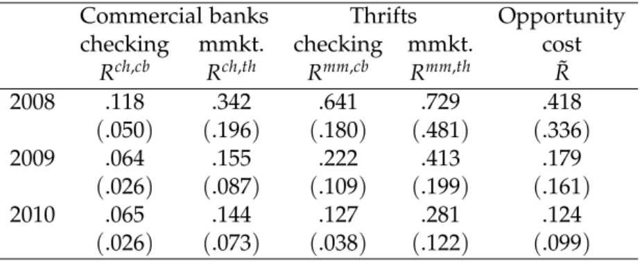
Commercial banks Thrifts Opportunity
checking mmkt. checking mmkt. cost
Rch,cb Rch,th Rmm,cb Rmm,th R˜ 2008 .118 .342 .641 .729 .418 (.050) (.196) (.180) (.481) (.336) 2009 .064 .155 .222 .413 .179 (.026) (.087) (.109) (.199) (.161) 2010 .065 .144 .127 .281 .124 (.026) (.073) (.038) (.122) (.099) Source:RateWatch
Table 3: Means and (standard deviations) of interest rate series in the estimation sample
Time-series estimates of the average account interest rates and opportunity cost are
shown in Table 3. As in Attanasio, Guiso, and Jappelli (2002), we find substantial
cross-sectional variation in interest rates that is helpful in identifying cash demand. The standard deviation of the interest-rate variables is around 50 percent (and more than one-third) of
the mean in every year.14 Figure6in Appendix Bshows that there is substantial variation
in our measure of the opportunity cost evenwithinstates. That is, our econometric
identi-fication of interest elasticity does not rely solely on interest rate differences across states or across years, but it also exploits the variation in interest rates across different types of bank accounts in a given state and year.
4
Cash inventory management
A staple of the U.S. payments markets, more so than in the rest of the world, is the widespread use of credit cards. Therefore this section will review an extension of the Baumol-Tobin model by Sastry (1970) (see also Lewis (1974)) that allows for the use of
credit cards.15 The analytical tractability of this model makes it an ideal tool to illustrate
the main point of this paper: The interest elasticity of cash demand changes with the in-terest rate paid on credit card debt. The presence of credit cards opens a new way for consumers to economize on cash holding costs: Paying for a larger fraction of transactions with credit card enables them to reduce cash holdings without a corresponding increase in the frequency of costly cash withdrawals. This strategy, however, becomes less attractive as interest rates paid on credit card debt increase.
In this version of the BT model consumers who run out of cash can keep transacting
at the marginal cost of the credit card borrowing rate, instead of paying the fixed cost of
14Part of this variation might come from different composition of accounts across states. For example, in richer states more people may hold checking accounts with high minimum balance requirements and corre-spondingly higher interest rates, which would give that state a high average checking account interest rate.
M M
T 0
D
Figure 3: Baumol-Tobin model with borrowing
The main difference compared to the BT model is that consumers can now go into debt. Withdrawals occur after cash holdings have been depleted, meaning that consumers accumulate some debt (D) during the process. At the moment of the withdrawal this debt is repaid, hence the cash balance after withdrawingWwill beM<W.
cash withdrawal. At the time of running out cash, themarginal cost of using cash for the
next transaction is infinite, so some credit use will always be optimal. However, the rising totalcost of using credit (credit card interest times the accumulated debt) will eventually outweigh the cost of using cash (fixed withdrawal cost plus forgone interest) if the credit card interest rate is higher than the interest earned on money kept at the bank.
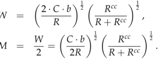
Formally, the problem can be stated as:16
minM,W,D R·M+b· C W +R cc·D, s.t. M = M 2 2W D= (W−M)2 2W ,
where M denotes average cash holdings, M denotes cash holdings after withdrawals, W
denotes the amount withdrawn (part of which is immediately spent on repaying the
out-standing balance on credit cards), andDdenotes average credit card debt over the period.
Note that this model nests the original BT model, whenD=0, that isW = M. In the case
with D>0, however, consumers have to make two decisions: how much cash to withdraw
(W) and how much debt to incur before a cash withdrawal (W−M).17 The solution for
withdrawals and cash holdings is
W = 2·C·b R 12 Rcc R+Rcc 12 , M = W 2 = C·b 2R 12 Rcc R+Rcc 12 .
As borrowing becomes prohibitively expensive, Rcc → ∞, these formulas collapse to the
square-root rule of the BT model. In general, however, the interest elasticity of cash holding
16For details about the model setup and solution see Sastry (1970).
17Since the model is deterministic, it is never optimal for the decisionmaker to withdraw cash before her cash holdings are depleted. As Alvarez and Lippi (2009) and Miller and Orr (1966) show, with a stochastic consumption flow individuals would get cash sooner, as a precaution against running out of cash and thereby forgoing a consumption opportunity.
becomes ∂M
∂R = −0.5
1+ R+RRcc
, meaning that the interest elasticity of cash demand is a function of the credit card interest rate. In particular, a higher credit card interest rate, ceteris paribus, leads to a lower interest elasticity (in absolute value). This is the implication of the model that we will test on our data.
Taking logs of the last equation yields
log(M) =0.5·log b 2 +0.5·log(C) +0.5·log(Rcc) −0.5·log(R(R+Rcc)), (1)
which is similar to the specification used in most of the microeconometric studies of cash demand. Unfortunately, the SCPC does not provide data on the interest paid on credit card debt, so we cannot estimate the above equation directly. We can, however, proxy for the credit card interest rate using information on credit card debt: Convenience users of credit cards (those who always pay off their full balance at the end of the billing cycle) pay no
interest on their current balance, while revolvers pay Rcc even for new purchases as soon
as their card is swiped at the register (with the exception of a few high-end credit cards). Hence the cash demand specification that our data allow us to estimate is:
log(Mit) =Xit0 γ+β1·log(Yit) +β2·log(Rit) +β3·log(Rit)×revolverit
+β4·revolverit+eit,
(2)
where Xit is a vector of proxies for the cost of withdrawing cash (b), a direct measure of
which is not available. Among these proxies are demographic variables, indicator variables for primary withdrawal method, and the share of cash transactions in the total number of
transactions.18 Nor do we have a direct measure of consumption expenditure (C), but will
use household incomeYitto proxy for that. revolveritdenotes if householdirevolves credit
card debt in yeart, we allow for this variable to have both a level effect on cash holdingsβ4
and an effect on the interest elasticity β3.
The error term, eit, has two sources: First, it accounts for individual heterogeneity not
observed by the econometrician. Second, there is likely to be measurement error in the de-pendent variables, resulting from the fact that the variables in our data do not correspond perfectly to their counterparts in the Baumol-Tobin model. For example, withdrawals mea-sure the usual amount withdrawn at the most frequently visited withdrawal location, not
from all locations.19 Although cash in wallet is measured more accurately, it may not
18The SCPC asks questions about the number of transaction in a typical month; information on the dollar value of these transactions is not collected. The value of cash transactions tends to be smaller on average than transactions made by other payment methods, as shown in Bagnall et al. (2013).
19Withdrawals also have a nonstandard distribution, in that it is a mixture of continuous distributions (result-ing from, say, withdrawals at the bank) and discrete distributions (ATM withdrawal). This means that the error in the regression with the usual withdrawal amount on the left-hand side is clearly not normally distributed,
correspond exactly to cash holdings used to finance everyday expenditures, as noted in
Section3.
4.1 Adoption of interest-bearing accounts and payment instruments
An implicit assumption behind the above model is that the decisionmaker has an
interest-bearing bank account and a credit card. However, as Table2 shows, this is not true for all
U.S. consumers. Moreover, the decision to open such an account or apply for a credit card is probably affected by the expected reduction in transactions costs that these instruments could provide for consumers. To correct for this self-selection, microeconometric studies of money demand model the adoption of bank accounts and payment instruments before the money demand equations are estimated.
The adoption decision for the interest-bearing checking account and credit card are
as-sumed to be separate choices.20 In both cases it is assumed to take the form of a cost-benefit
analysis, as in Mulligan and Sala-i-Martin (2000) and Attanasio, Guiso, and Jappelli (2002). The benefits can be thought of as interest income, or as less time spent with completing transactions, while the costs usually include setup costs and use or maintenance costs (for example, monthly account or card fees, minimum balance requirements). Data are available on some of these factors, such as financial wealth and interest rates. Other inputs of the adoption decision, such as the time it takes to understand the workings of a new payment instrument, are not measured directly and will be proxied with demographic variables. If the net benefits, benefits minus costs, are positive the individual will choose to adopt an instrument: z∗it=θ0+θ1·Yit+θ2·wealthit+θ30Rchst,cb+θ 0 4X˜it+θ50Ait+ci+νit (3) zit= ( 1 z∗it>0 0 z∗it≤0 ,
where zit is a binary variable indicating adoption of an interest-bearing bank account or
credit card,z∗itis a continuous latent variable measuring the net benefit of adoption,Yit
de-notes family income, Rchst,cb measures the prevailing commercial bank checking account
in-terest rate in respondenti’s state of residence, ˜Xitis a vector of demographic characteristics,
Aitis a vector of the respondent’s assessments of the acceptance, security, and cost of credit
cards relative to debit cards and cash, andci+νitis a composite error term that includes an
individual-specific random effect,ci, and a component that varies across both individuals
and time periods, νit. We interpret the error term as the sum of all other factors that
but the central limit theorem still applies; hence our estimates are asymptotically normally distributed. 20See Koulayev et al. (2012) for a model with more payment instruments, where individuals adopt a portfolio of payment instruments and take into account the substitutability and complementarity of all the instruments simultaneously.
are known to the decisionmaker, but not to the econometrician, as in Chapter 2 of Train (2009), and assume that it is independent of all other explanatory variables and follows a
standard normal distribution.21 The variables that are included in the selection equations,
equation (3), but not in the cash demand regressions are: the ratio of bank branches to
pop-ulation at the state level and indicator variables for race, education, respondents’ income rank within the household, home ownership, and being born outside the U.S.
Using the inverse Mills ratios from the probit equations for credit card and interest–
bearing account adoption22in the second-stage regressions will eliminate the potential
self-selection bias. The second-stage equation becomes,
log(Mit) =β0+τ2009+τ2010+β1·log(Yit) +β2·log(R˜it) +β3·log(R˜it)×revolverit
+β4·log(R˜it)×branchesit+γ0Xit+ρ0λit+εit,
(4)
where Mi denotes one of the three cash variables of interest (the “usual amount of cash
withdrawal at primary location” or the number of withdrawals or cash in wallet); (τt)
is a time-varying intercept; ˜Rit denotes the alternative cost of holding cash; Yit denotes
household income (a proxy for cash spending);Xit denotes individual characteristics that
serve as proxies for the parameters in the BT model;23 and λit is a vector of the inverse
Mills ratios computed from equation (3). Inclusion of the inverse Mills ratios means that
the error term in equation (4), εit, is independent of the composite errors in the adoption
equations and has a mean of zero.24
5
Estimation method
The sample and the system of equations to be estimated (two adoption equations and the
cash demand equation, equations (3) and (4)) require some modifications to the Heckman
(1979) procedure. Other than these adjustments, the methods used in this paper are similar to those in a number of recent cash demand estimations, such as Lippi and Secchi (2009).
The first adjustment to the Heckman (1979) procedure is necessitated by respondents who appear in more than one wave of the survey. The SCPC tries to maintain a panel of respondents, so many of them appear in more than one wave of the survey (for details on
21
νita,νitc (where superscriptsa,c denote the equation for interest-bearing account and credit card adoption,
respectively) are assumed to be serially uncorrelated and follow a standard normal distribution, whilecai, cci are normally distributed with mean zero and varianceσc2a
i andσ 2 cc
i, respectively. The error terms in the adoption equations (cai,νita,cci,νcit) are assumed to be uncorrelated with each other. Potential self-selection means that the
error term in equation (2),eit, might be not be independent of the composite error termscai+νait,cci+νitc. 22Computation of the inverse Mills-ratios takes into account that there are two sources of unobserved hetero-geneity in the adoption equations:ciandνit; therefore,zit∗ is normally distributed with varianceσc2+σν2, where σ2νis normalized to 1.
23For the full list please refer to Table7in AppendixA. 24This is true under the assumption thatE
eit|z∗it a,z∗
it c
this see Table 9 Appendix B).25 This nonrandomness of the sample would already cause the standard errors of a simple ordinary least-squares (OLS) regression to be incorrect, but it raises an additional issue in our application. Adoption decisions are likely to be highly correlated over time for the same respondent: Somebody with a credit card in 2008 is likely to have a credit card in 2009 as well. To take this autocorrelation over time into account (for the panel observations), random effect probit models were estimated in the first stage.
In both cases, the estimated autocorrelation in the composite errors,ci+νit in equation (3),
was highly significant both statistically and economically (see Table4).
We used the two-step version of the Heckman (1979) estimator: First estimating the (random effect) probit equations for interest-bearing account and credit card adoption, then using the resulting inverse Mills ratios as explanatory variables in the cash demand equa-tion (second step) estimated with OLS. The presence of generated regressors (the inverse Mills ratios) does not affect the consistency of the OLS estimator, but it causes the OLS stan-dard errors to be biased (even independently from the nonrandomness issue noted above). Following Lippi and Secchi (2009), we correct for the biased standard errors by bootstrap-ping, using 1,000 repetitions. Given the presence of repeat respondents in the sample, the bootstrapping procedure itself is not entirely straightforward. Instead of bootstrapping the observations, we bootstrappedindividuals, thus making sure that the composition of every bootstrap sample remained the same as the original one in terms of the number of respon-dents from each year, pair, or triplet of years.
Since our sample is relatively small and shrinks further due to missing or zero observa-tions, we estimated the second-stage equations on a pooled cross-section of all households
from the three waves of the survey.26
6
Results
6.1 Adoption equation
The adoption equations for interest–bearing accounts and credit cards are presented in
Table4. The reported numbers are the marginal effects computed at the sample means.
The predictive power of the model of interest–bearing account ownership is quite low,
with a pseudo-R2of about 0.05. Adoption is affected significantly only by income, financial
25This structure is not unique to the SCPC. For example, the SHIW data also have a subset of respondents who are surveyed in multiple waves.
26To check the robustness of the findings, we dropped the 306 panel observations from 2009, re-ran the estimations, and got similar results. In another robustness check, we kept only the panelists and re-ran the estimations using OLS in the second stage and again found similar results. With a fixed-effect estimator on the panel sample the results changed markedly; the point estimates became mostly insignificant. Since we have only two observations per respondent to estimate individual fixed effects, we do not take this result as conclusive evidence against our specification and plan to revisit the issue of panel estimation once additional data become available.
Interest–bearing account Credit card log(Income) .018∗∗∗ (.005) .047∗∗∗ (.006) log(Wealth) .003∗∗ (.002) .006∗∗∗ (.002) Age −.000 (.000) .002∗∗∗ (.000) Latino .004 (.014) −.018 (.016) Black .005 (.012) −.055∗∗∗ (.013) Male −.002 (.006) −.011 (.008)
Less than high-school educated −.040∗∗ (.021) −.076∗∗∗ (.024)
High-school educated −.020∗∗ (.009) −.044∗∗∗ (.009)
Single −.011 (.011) .006 (.013)
Married −.005 (.009) .002 (.010)
Number of household members −.003 (.002) −.012∗∗∗ (.003)
Employed .007 (.008) −.019∗ (.010) Unemployed −.008 (.013) −.026∗ (.015) Disabled −.010 (.015) −.077∗∗∗ (.017) Self-employed −.010 (.010) .016 (.013) Income rank: 1st .011 (.011) .039∗∗∗ (.012) Income rank: 2nd .011 (.013) .034∗∗ (.014) Income rank: 3rd .007 (.011) .010 (.012) Homeowner .025∗∗∗ (.009) .025∗∗∗ (.008) Born abroad −.022∗ (.012) .049∗∗∗ (.019)
Branches (per 1000 residents) .023 (.021) .026 (.025)
Year 2009 −.010 (.008) −.004 (.008)
Year 2010 −.014∗ (.008) −.024∗∗∗ (.008)
log(commercial bank checking rate) .004 (.007) −.007 (.008)
Cost .019∗∗∗ (.006) Security .011∗ (.006) Acceptance .059∗∗∗ (.015) Share ofσc2+σν2 explained by RE .663 .885 p-value of H0 :σc2 =0 .000 .000 Pseudo R2 .051 .193 Observations 3,728 3,738
Marginal effects. Standard errors in parenthesis.
wealth, education, and homeownership. The probability of account adoption increases by 1.8 percent after a 1 percent increase in income and by 0.3 percent after a similar change in wealth. The marginal effect of having less than a college education is of roughly the same magnitude as a 1 percent decrease in income for high-school gradualtes and equivalent to about a 2 percent decrease in income for high-school dropouts, compared with college graduates (omitted category). Homeownership raises the probability of account adoption by 2.5 percent. Other studies on bank account adoption, for example Schuh and Stavins (2012) and Hogarth, Anguelov, and Lee (2005), also found significant effects of socioeco-nomic variables, although the explanatory power of Schuh and Stavins (2012) is similar to ours. More importantly for the money demand literature, unlike in Mulligan and Sala-i-Martin (2000), interest rates do not affect interest–bearing account adoption, although, as
noted earlier in footnote 9, a direct comparison with their results is difficult, due to the
different definitions of interest–bearing accounts. The random–effects component (ci in
equation (3)) is highly significant, justifying the choice of the econometric specification.
Credit card adoption is better explained by our model, as evidenced by the pseudo-R2
of 0.19. It is also heavily influenced by income: A 1 percent increase in income leads to a 4.7 percent increase in the probability of credit card adoption. The effect of financial wealth and education on credit card adoption is about twice as large as on interest–bearing account adoption. African-Americans are 5.5 percent less likely to have credit cards than white people (omitted category). Bigger households are also less likely to have credit cards and so are disabled people. Income ranking within the family also matters: breadwinners are more likely to own credit cards. Home ownership and being born abroad both increase the likelihood of having a credit card. Acceptance and the cost of using credit cards are both important for the adoption decision. Credit card adoption is unaffected by the interest rates on checking accounts. It would be interesting to see how credit card interest rates affect credit card adoption, but we have no data on this. What is interesting from this result, however, is that if credit card interest rates affect adoption, it has to be the result of changes in those rates that are orthogonal to checking account rates. We find evidence of a significant decrease in credit card adoption in 2010 compared with the previous two years, and again the random–effects term plays an important role in explaining the autocorrelation of the adoption decision over time for the same respondent.
6.2 Cash demand equations
The next subsections discuss the results of the cash-demand estimation using (the loga-rithms of) withdrawal amounts, cash in wallet, and number of withdrawals as the depen-dent variables. The reported regressions were estimated on a subsample of respondepen-dents with interest–bearing account and credit cards; depending on the number of available ob-servations on the left-hand side variable, the estimation samples consist of 2,363 to 2,440
observations.
Tables 5 and6 contain five different models using, separately, the withdrawal amount
and cash in wallet as the dependent variable, with our preferred specification in the last column. As the tables show, most of the point estimates are fairly robust to the various
specifications. The full estimation output is reported in Table7in AppendixA.
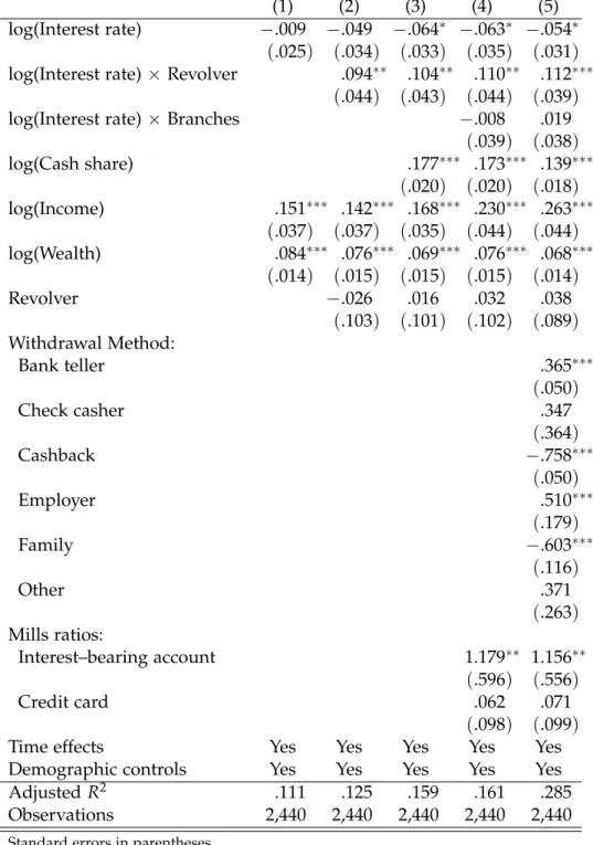
6.2.1 Cash withdrawals
The first two columns highlight the main finding of the paper. The first column in
Ta-ble 5 can be interpreted as a test of the original BT model without distinguishing
be-tween revolvers and convenience users. (All regressions, however, control for demographic
characteristics and include year and month fixed effects.27) The second column controls for
this difference using the “revolver" indicator variable and its interaction with the opportu-nity cost of holding cash.
While the first model finds highly significant effects of income and financial wealth on usual cash withdrawals with the expected positive sign and sensible magnitude, it fails to identify a significant interest elasticity. The second column shows that the failure to do so could be the result of restricting the interest elasticity of convenience users and revolvers
to be the same. As predicted by the model in Section4, the interest elasticity of revolvers
is significantly bigger (not in absolute value) than that of convenience users. While the
interest elasticity of convenience users is never significantly different from zero (at the 5 percent level), the point estimate is remarkably close to what Lippi and Secchi (2009) found on recent data for Italy and is in line with the theoretical model of Alvarez and Lippi (2009), which predicts that the interest elasticity of cash demand goes to zero as the interest rate approaches zero. Remarkably, Daniels and Murphy (1994) estimated a small but significantly positive interest elasticity of cash demand for the United States using data from the mid-1980’s. While they noted that credit card use might explain this finding, their data did not allow controlling for differences in credit card interest rates.
Adding a measure of cash use intensity (share of the number of cash transactions in total transactions) to the list of explanatory variables in the third column changes little of the qualitative results, although the variable itself is highly significant. Correcting for self-selection, in column 4, causes the income elasticity to increase substantially, but has little effect otherwise, mostly because the Mills ratios do not appear to be very significant. This specification also borrows from Lippi and Secchi (2009) and allows for the interest elasticities to differ by the number of bank branches per capita (measured at the state level),
but this seems to make little difference in our sample.28
27While most of the responses for the SCPC arrive in October, some respondents fill out the surveys later. In 2009, in particular, many responses were recorded in November.
28Note that for ATM card holders this variable was also insignificant in Lippi and Secchi (2009) and, as shown in Table2, about 90 percent of our estimation sample have a debit or ATM card.
(1) (2) (3) (4) (5)
log(Interest rate) −.009 −.049 −.064∗ −.063∗ −.054∗
(.025) (.034) (.033) (.035) (.031)
log(Interest rate)×Revolver .094∗∗ .104∗∗ .110∗∗ .112∗∗∗
(.044) (.043) (.044) (.039)
log(Interest rate)×Branches −.008 .019
(.039) (.038) log(Cash share) .177∗∗∗ .173∗∗∗ .139∗∗∗ (.020) (.020) (.018) log(Income) .151∗∗∗ .142∗∗∗ .168∗∗∗ .230∗∗∗ .263∗∗∗ (.037) (.037) (.035) (.044) (.044) log(Wealth) .084∗∗∗ .076∗∗∗ .069∗∗∗ .076∗∗∗ .068∗∗∗ (.014) (.015) (.015) (.015) (.014) Revolver −.026 .016 .032 .038 (.103) (.101) (.102) (.089) Withdrawal Method: Bank teller .365∗∗∗ (.050) Check casher .347 (.364) Cashback −.758∗∗∗ (.050) Employer .510∗∗∗ (.179) Family −.603∗∗∗ (.116) Other .371 (.263) Mills ratios: Interest–bearing account 1.179∗∗ 1.156∗∗ (.596) (.556) Credit card .062 .071 (.098) (.099)
Time effects Yes Yes Yes Yes Yes
Demographic controls Yes Yes Yes Yes Yes
AdjustedR2 .111 .125 .159 .161 .285
Observations 2,440 2,440 2,440 2,440 2,440
Standard errors in parentheses
∗ p<0.10,∗∗ p<0.05,∗∗∗ p<0.01
Finally, the benchmark model in the last column allows for the most preferred cash withdrawal method to have a level effect on the (log of) the amount withdrawn. Com-pared with ATM users (omitted category), people who get cash at the bank teller or from their employer tend to withdraw 36.5 and 51.0 percent more cash, respectively. Getting cash from family members or as cash back at a retail store, on the other hand, leads to smaller withdrawal amounts by 60.3 and 75.8 percent, respectively. These findings extend the results from recent cash demand estimations, such as Lippi and Secchi (2009) and Stix (2004), which found significant negative effects of ATM networks on cash withdrawals and holdings compared with other locations. While adding these variables nearly doubles the
adjustedR2 of the regression, they have very little effect on the income, wealth, or interest
elasticities.
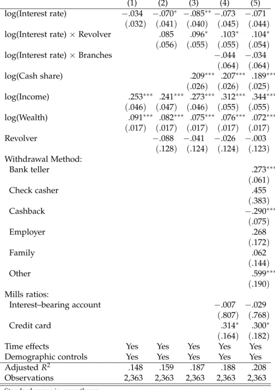
6.2.2 Cash holdings in purse, pocket and wallet
Table 6 shows analogous results with the log of cash in wallet as the dependent variable.
The main difference compared to Table5 is the significance level of the interest elasticity
estimates, primarily due to more imprecisely estimated coefficients. The revolver interac-tion term only turns significant at the 10 percent level once we control for the share of cash transactions, although the point estimates are comparable to those in the withdrawal amount regression. The primary withdrawal location variables seem to matter a little less for cash holdings than they do for withdrawals, possibly showing that respondents use more than one source of cash frequently. In fact, according to the SCPC, about one third of the withdrawals happen at the secondary source. In general, the explanatory power
of these regressions is lower than for primary withdrawals, with the adjusted R2 at 0.208
compared to 0.285 in the specification for withdrawal amount.
6.2.3 Number of withdrawals
Note that in the BT model the interest elasticity of the number of withdrawals is the inverse of the interest elasticity of the withdrawal amount, since the number of withdrawals is the
ratio of total cash expenditure and the withdrawal amount.29 The estimations results are
displayed in Table7. While the estimated interest elasticities have the predicted signs, they
are insignificant. Income and cash share elasticities are in line with the estimates obtained in the other regressions, but the sign of the financial wealth variable is the opposite of what we expected. All in all, this specification performs the worst, consistent with our prior that respondents’ recall of the number of withdrawals is probably less precise than their recall of the usual amount they withdraw.
29This is the source of the welfare cost of inflation: higher nominal interest rates result in more withdrawals, which involve a fixed resource cost.
(1) (2) (3) (4) (5)
log(Interest rate) −.034 −.070∗ −.085∗∗−.073 −.071
(.032) (.041) (.040) (.045) (.044)
log(Interest rate)×Revolver .085 .096∗ .103∗ .104∗
(.056) (.055) (.055) (.054)
log(Interest rate)×Branches −.044 −.034
(.064) (.064) log(Cash share) .209∗∗∗ .207∗∗∗ .189∗∗∗ (.026) (.026) (.025) log(Income) .253∗∗∗ .241∗∗∗ .273∗∗∗ .312∗∗∗ .344∗∗∗ (.046) (.047) (.046) (.055) (.055) log(Wealth) .091∗∗∗ .082∗∗∗ .075∗∗∗ .076∗∗∗ .072∗∗∗ (.017) (.017) (.017) (.017) (.017) Revolver −.088 −.041 −.026 −.003 (.128) (.124) (.124) (.123) Withdrawal Method: Bank teller .273∗∗∗ (.061) Check casher .455 (.383) Cashback −.290∗∗∗ (.075) Employer .268 (.172) Family .062 (.144) Other .599∗∗∗ (.190) Mills ratios: Interest–bearing account −.007 −.029 (.807) (.768) Credit card .314∗ .300∗ (.164) (.182)
Time effects Yes Yes Yes Yes Yes
Demographic controls Yes Yes Yes Yes Yes
AdjustedR2 .148 .159 .187 .188 .208
Observations 2,363 2,363 2,363 2,363 2,363
Standard errors in parentheses
∗ p<0.10,∗∗ p<0.05,∗∗∗ p<0.01
6.3 Robustness
One potential objection to the identification is that the share of cash transactions in total transactions may be endogenous to cash withdrawals or cash holdings. To alleviate these
concerns, Table8 presents the GMM distance statistics for the test of the exogeneity of the
cash share variable, as implemented by the ivreg2 command of Stata; for example, see
Baum, Schaffer, and Stillman (2007).
For both withdrawal amounts and cash in wallet as the dependent variable the test cannot reject the null hypothesis that the (log of) cash share variable is exogenous in our benchmark model. The test compares our benchmark model with one that treats (the log of) the cash share variable as endogenous and instruments it using respondents’ self-reported
assessment of security and cost of cash relative to credit and debit cards (see AppendixB
for details on how these measures were constructed). The Hansen J-test indicates that the instruments were rightfully excluded from the cash demand regressions, while the GMM distance statistics show that the model where cash share is instrumented for yields similar estimates to our benchmark specification, that is, the model that is consistently estimated is not significantly different from the model that was suspected of being inconsistently estimated due to the potential endogeneity of the cash share variable.
7
Implications for the welfare cost of inflation
Our estimation reveals economically and statistically significant differences in the inter-est elasticity of cash demand by credit card users with different borrowing behavior and
opportunity costs. Figure 4 illustrates the results in two ways that portray the potential
implications for the welfare cost of inflation associated with the currency portion of money.
The left panel of Figure 4 plots estimated cash demand functions for revolvers and
convenience users from the regression results for cash in wallet. The demand function for convenience users exhibits the standard, negative, nonlinear shape that is consistent with previous estimation of money demand. As explained in Robert E. Lucas (2000) and Ireland (2009), the welfare cost of inflation associated with this demand equals the total area under this demand curve less seigniorage revenue at the steady-state nominal interest rate (real rate plus expected inflation). In sharp contrast, the estimated function for revolvers is essentially vertical—having a slight positive but statistically insignificant slope—revealing interest-inelastic cash demand. Therefore, the area “under” the revolvers’ demand curve is much smaller, and revolvers do not substitute away from cash when the interest rate (or inflation) increases. Aggregate welfare loss depends on the relative weight of revolvers in
the population, which Table2 showed is nearly one third of U.S. adults based on SCPC
data, so the impact is not trivial.
0
3
6
9
Nominal interest rate
70 80 90 100 110 120 Cash in wallet ($) Revolvers Convenience users 0 3 6 9
Nominal interest rate
70 80 90 100 110
Cash in wallet ($) Combined cash demand Joint estimate
Figure 4: Cash demand function of convenience users and revolvers (left) and average cash demand with and without accounting for revolvers (right)
two estimated cash demand functions stemming from different treatments of the underly-ing heterogeneity in the data. The longer-dashed line represents the weighted average of the demand functions in the left panel, where the weight is the share of revolvers in the estimation sample. The shorter-dashed line is the demand function from a regression that uses the same estimation sample but does not control for the microeconomic heterogeneity of cash behavior. In particular, it restricts the interest elasticity to be the same for revolvers and convenience users, making the homogeneous-consumer regression susceptible to ag-gregation bias. Indeed, the demand function for the homogeneous-consumer regression is shifted significantly to the right of the demand function that accommodates micro hetero-geneity. Here, one can easily see the main implication—accounting for micro heterogeneity lowers the welfare cost of inflation by shifting the cash demand curve to the left and re-ducing the area under the demand curve. Previous studies on the welfare cost of inflation that did not account for different interest elasticities, such as Cooley and Hansen (1991), Gillman (1993), Dotsey and Ireland (1996), and Khan, King, and Wolman (2003), may also have overestimated the welfare cost of inflation.
Our regression results may also have implications for the debate between Robert E. Lu-cas (2000) and Ireland (2009). Estimation of our model using the semi-log specification advocated by Ireland produced insignificant estimates of the interest elasticity and poorer fit overall (results not reported here). This finding, combined with the relative success of our log-log specification, motivates an examination of the model specification issue using