A NEURAL NETWORK APPROACH TO BORDER GATEWAY PROTOCOL PEER FAILURE DETECTION AND PREDICTION
A Thesis Presented to
the Faculty of California Polytechnic State University San Luis Obispo
In Partial Fulfillment
of the Requirements for the Degree Master of Science in Computer Science
by Cory B. White December 2009
c
2009
Cory B. White ALL RIGHTS RESERVED
COMMITTEE MEMBERSHIP
TITLE: A Neural Network Approach to Border
Gateway Protocol Peer Failure Detection and Prediction
AUTHOR: Cory B. White
DATE SUBMITTED: December 2009
COMMITTEE CHAIR: Franz Kurfess, Ph.D.
COMMITTEE MEMBER: Hugh Smith, Ph.D.
Abstract
A Neural Network Approach to Border Gateway Protocol Peer Failure Detection and Prediction
Cory B. White
The size and speed of computer networks continue to expand at a rapid pace, as do the corresponding errors, failures, and faults inherent within such extensive networks. This thesis introduces a novel approach to interface Border Gateway Protocol (BGP) computer networks with neural networks to learn the precursor connectivity patterns that emerge prior to a node failure. Details of the design and construction of a framework that utilizes neural networks to learn and mon-itor BGP connection states as a means of detecting and predicting BGP peer node failure are presented. Moreover, this framework is used to monitor a BGP network and a suite of tests are conducted to establish that this neural network approach as a viable strategy for predicting BGP peer node failure. For all per-formed experiments both of the proposed neural network architectures succeed in memorizing and utilizing the network connectivity patterns. Lastly, a discussion of this framework’s generic design is presented to acknowledge how other types of networks and alternate machine learning techniques can be accommodated with relative ease.
Acknowledgements
I am greatful for having a dedicated and reliable committee of professors who were always willing to discuss my progress and offer constructive suggestions. Thanks specifically to the chair of my committee–my mentor–Dr. Franz Kur-fess. His guidance, interests, and eager enthusiasm provided me with a strong motivation to explore the field of artificial intelligence and machine learning. He has always maintained an optimistic sense of humor and has been understanding and more than willing to work with me through any difficulties. His devotion to the interests and paths of his students–myself being no exception–is exceptional. Thank you for being such a great teacher, mentor, and friend.
Also, a very special thanks to my parents and grandparents. Throughout my college experience, these members of my familiy have provided me with economic stability, confidence, understanding, guidance, and always a listening ear during the tougher times. Their self-sacrifice and selfless continual support have sculpted me into the person I am today and has allowed me to accomplish my college goals and earn this Master’s degree. My accomplishments as a son reflect their successes as a family unit. Thank you for all that you have given.
Contents
Contents vi
List of Tables x
List of Figures xi
List of Code Blocks xiv
1 Introduction 1
1.1 Overview of Problem Statement . . . 1
1.2 Outline. . . 3
2 Related Work and Background 4 2.1 Neural Networks . . . 4
2.1.1 A Brief History . . . 4
2.1.2 Neural Networks As Predictive Tools . . . 6
2.2 The Border Gateway Protocol . . . 7
2.2.1 BGP Monitoring Tools . . . 10
2.2.2 Network Monitoring Tools Utilizing Machine Learning . . 11
3 Domain Details 17 3.1 BGP and SNMP . . . 17
3.2.1 Biological Inspiration . . . 20
3.2.2 The Backpropagation Learning Algorithm . . . 23
3.2.3 Architectural Design Decisions. . . 27
4 Design and Implementation 29 4.1 High-Level Concept Design. . . 29
4.1.1 Utilizing Neural Networks . . . 29
4.1.2 Training Data Collection Methodology . . . 32
4.2 Software Implementation Details . . . 35
4.2.1 The User Interface . . . 35
4.2.2 Relevant Configuration Options . . . 40
4.2.3 Backend Programmatic Details . . . 45
5 Experiments 58 5.1 Test Suite . . . 58
5.2 Experimental Network 1 . . . 59
5.2.1 General Neural Network Implementation . . . 61
5.2.2 Expert Neural Network Implementation . . . 66
5.3 Experimental Network 2 . . . 73
5.3.1 General Neural Network . . . 78
5.3.2 Expert Neural Network . . . 84
5.4 Experimental Network 3 . . . 92
5.4.1 General Neural Network . . . 94
5.4.2 Expert Neural Network . . . 98
6 Results and Conclusions 108
7.1 Extending the BGPNNF . . . 111 7.2 Other Machine Learning Techniques. . . 112 7.3 Other Networks . . . 113
Appendices 119
A Neural Network Comparisons 119
A.1 Neural Networks for Five Router Full Mesh. . . 120 A.2 Neural Networks for Forty Router Full Mesh . . . 120 A.3 Neural Networks for Ten Router Sparsely Connected . . . 123
List of Tables
3.1 Representative BGP Speaker Numbers . . . 18 4.1 XOR Truth Table . . . 52 5.1 Experiment 1 Trained General Neural Network Output for Router
SDND . . . 63 5.2 Experiment 1 Trained General Neural Network Output for Router
EDND . . . 65 5.3 Experiment 1 Trained General Neural Network Output for Router
Completely Down . . . 71 5.4 Experiment 1 Trained Expert Neural Network Output for Router
SDND . . . 72 5.5 Experiment 1 Trained Expert Neural Network Output for Router
EDND . . . 72 5.6 Experiment 1 Trained Expert Neural Network for Router
Com-pletely Down . . . 73 5.7 Experiment 2 Trained General Neural Network Output for Router
SDND . . . 81 5.8 Experiment 2 Trained General Neural Network Output for Router
EDND . . . 82 5.9 Experiment 2 Trained General Neural Network Output for Router
5.10 Experiment 2 SDND Prediction with General Neural Network . . 84 5.11 Experiment 2 EDND Prediction with General Neural Network . . 85 5.12 Experiment 2 Correlated Prediction with General Neural Network 85 5.13 Experiment 2 Expert Training Information . . . 86 5.14 Experiment 2 Expert Neural Network Output for Router SDND . 88 5.15 Experiment 2 Expert Neural Network Output for Router EDND . 89 5.16 Experiment 2 Expert Neural Network Output for Router
Com-pletely Down . . . 90 5.17 Experiment 2 SDND Prediction with Expert Neural Networks . . 91 5.18 Experiment 2 EDND Prediction with Expert Neural Networks . . 91 5.19 Experiment 2 Correlated Prediction with Expert Neural Networks 92 5.20 Experiment 3 Trained General Neural Network Output for Router
SDND . . . 96 5.21 Experiment 3 Trained General Neural Network Output for Router
EDND . . . 97 5.22 Experiment 3 Trained General Neural Network Output for Router
Completely Down . . . 98 5.23 Experiment 3 Trained Expert Neural Network Output for Router
SDND . . . 103 5.24 Experiment 3 Trained Expert Neural Network Output for Router
EDND . . . 104 5.25 Experiment 3 Trained Expert Neural Network Output for Router
List of Figures
2.1 The BGP FSM . . . 9
3.1 Full Mesh vs. Route Reflection iBGP . . . 19
3.2 A Biological Neuron . . . 20
3.3 Connected Biological Neurons . . . 21
3.4 The Biological Neuron and Mathematical Counterpart . . . 21
3.5 The Neuron Core . . . 22
3.6 Activation Functions . . . 22
3.7 Feedforward Neural Network . . . 23
3.8 The Training Loop . . . 24
3.9 Training Error Surface . . . 25
3.10 Exemplary Neural Network Utilization . . . 26
3.11 The Two Neural Network Architectures Utilized . . . 28
4.1 Simple BGP Network . . . 30
4.2 Interfacing the iBGP Network with an Adjacency Matrix . . . 31
4.3 Interfacing the iBGP Adjacency Matrix to a Neural Network . . . 32
4.4 BGP Connection Failure Example . . . 33
4.5 Adjacency Matrix to Neural Net Example . . . 33
4.6 The BGPNNF User Interface . . . 36
4.7 Color Example of the BGPNNF User Interface . . . 37
4.9 Load Dialog User Interface. . . 38
4.10 New Neural Net User Interface. . . 39
4.11 Train Button User Interface. . . 40
4.12 The Input Test Network User Interface . . . 41
4.13 Five-Node Network . . . 42
4.14 The BGPNNF Flow Diagram . . . 46
4.15 XOR Neural Network . . . 52
5.1 The First Experimental Network . . . 60
5.2 Exemplary Patterns Memorized . . . 60
5.3 Correlated Router Down Pattern . . . 61
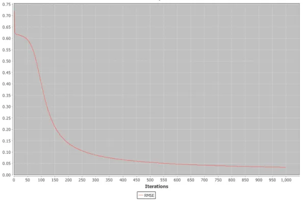
5.4 Experiment 1 General Neural Network Training RMSE . . . 62
5.5 An Example of SDND . . . 64
5.6 An Example of EDND . . . 65
5.7 Example Router Completely Down . . . 66
5.8 Experiment 1 EDND Prediction with General Neural Network . . 67
5.9 Experiment 1 SDND Prediction with General Neural Network . . 68
5.10 Experiment 1 Correlated Prediction with General Neural Network 69 5.11 Experiment 1 RMSE vs. Iterations for Each Expert Neural Network 70 5.12 Experiment 1 EDND Prediction with Expert Neural Networks . . 74
5.13 Experiment 1 SDND Prediction with Expert Neural Networks . . 75
5.14 Experiment 1 Correlated Prediction with General Neural Network 76 5.15 Large Fully-Connected Network. . . 77
5.16 Experiment 2 General Neural Network Failed Training RMSE . . 79
5.17 Experiment 2 General Neural Network Successful Training RMSE 80 5.18 Experiment 2 Expert RMSE Graphs . . . 87
5.20 Experiment 3 First General Training . . . 95
5.21 Experiment 3 Second General Training . . . 96
5.22 Experiment 3 EDND Prediction with General Neural Network . . 99
5.23 Experiment 3 SDND Prediction with General Neural Network . . 100
5.24 Experiment 3 Correlation Prediction with General Neural Network 101 5.25 Experiment 3 RMSE vs. Iterations for Each Expert Neural Network102 5.26 Experiment 3 EDND Prediction with Expert Neural Networks . . 105
5.27 Experiment 3 SDND Prediction with Expert Neural Networks . . 106
5.28 Experiment 3 Correlation Prediction with Expert Neural Networks 107 7.1 Two Exemplary Network Topologies . . . 114
7.2 More Exemplary Network Topologies . . . 114
7.3 Additional Exemplary Network Topologies . . . 115
7.4 Still More Exemplary Network Topologies . . . 116
7.5 Exemplary On-Chip Power Grid Network Model . . . 117
7.6 Three-Phase, Breaker-Oriented IEEE 24-Substation Reliability Test System . . . 118
A.1 Neural Network Training Comparisons for the Five Router Full Mesh121 A.2 Neural Network Training Comparisons for the Forty Router Full Mesh . . . 122
A.3 Neural Network Training Comparisons for the Sparse Network Topology. . . 124
List of Code Blocks
4.1 Example Node XML Element and Contents . . . 42
4.2 Example Router Configuration . . . 43
4.3 Example neuralNet Element for Configuring a General Neural Network 44 4.4 Example neuralNet Element for Configuring an Expert Neural Network 44 4.5 Example Configuration of the historyQueue . . . 45
4.6 NodeInfo Private Variables. . . 46
4.7 SNMP Poller Main Loop. . . 47
4.8 The createNodeDownList Method . . . 49
4.9 The nodeDownCheck Method . . . 50
4.10 The OQueue’s lookback Method . . . 50
4.11 The initNeuralNet Method . . . 51
4.12 The XOR Training Data . . . 52
4.13 Creating the IP Map for the CoreModel’s Internal Matrix . . . 54
4.14 CoreModel Update Method. . . 56
Chapter 1
Introduction
This chapter provides an exposition of the objectives of this thesis and the layout for the remainder of the document.
1.1
Overview of Problem Statement
The size and speed of computer networks continue to expand at a rapid pace, as do the corresponding errors, failures, and faults inherent within extensive networks. With this growth, large Internet-based companies such as Amazon, Google, and Yahoo! and even smaller companies with high reliance upon a com-puting infrastructure depend upon the reliability of such networks in order to earn revenue and remain dominant in competitive markets. Thus, the need grows for network tools and techniques to maintain and monitor such systems in order to quickly and efficiently detect problems and potentially even predict issues before they occur. These tools must therefore ascertain and store knowledge about the network topology and communication between nodes in order to draw inferences about any potential problems that may arise.
The specific protocol of interest is the Border Gateway Protocol (BGP). Ac-knowledged as the de facto interdomain routing protocol of the Internet, if a BGP router becomes jeopardized or goes offline,
An autonomous system can have its traffic black-holed or other-wise misrouted, and packets to or from it can be grossly delayed or dropped altogether. Malfunctioning ASes harm their peers by forcing them to recalculate routes and alter their routing tables...these events can disrupt international backbone networks and have the potential to bring a large part of the Internet to a standstill.[16]
This thesis introduces a novel approach to interface BGP computer networks with neural networks to learn the precursor connectivity patterns that emerge prior to a router failure. Such patterns are collected and then memorized by neural networks which will then be able to detect or, potentially, even predict future node failures if similar connective patterns emerge in the future. The co-founder of the Artificial Intelligence Laboratory of the Massachusetts Institute of Technology Marvin Minsky stated in 1991 that,
To program today, we must describe things very carefully, because nowhere is there any margin for error. But once we have modules that know how to learn, we won’t have to specify nearly so much–and we’ll program on a grander scale, relying on learning to fill in the details.[56]
This thesis demonstrates how neural networks can fill in the details necessary for subset of problems that can emerge within a computer network. Thus, the work presented here takes another step in the direction that Minksy predicted eighteen years ago.
1.2
Outline
This thesis will first acknowledge the background of neural networks, their wide range of application, and their popular use as predictive tools. Next, some relevant details of BGP will be presented along with a survey of current network monitoring tools and techniques that utilize machine learning techniques will be discussed. After the survey, a more in-depth look at BGP and the particular neu-ral network learning algorithm utilized in this thesis will be assessed. Following these details, the specific design applied in this thesis will be presented in both a high-level perspective as well as the details of the lower-level software framework implementation. Next, three representative network topologies will be considered and tested using the written software, which will be followed by corresponding results and conclusions. Lastly, a discussion of a wide range of potential future work stemming from this thesis will be conducted.
Chapter 2
Related Work and Background
This chapter will assess work that is related to the content of this thesis. The following sections will cover a brief history of neural networks, their use as predictive tools, some relevant details on BGP, and network monitoring tools.
2.1
Neural Networks
This section will introduce a brief history of neural networks as well as provide various examples of how neural networks have been used as predictive tools.
2.1.1
A Brief History
Artificial neural networks provide a new approach to solving ill-structured problems that are not easily solved using procedural solutions. Neural networks are composed of nodes, or neurons, that perform in a manner similar to that of the biological neuron along with interconnecting weights between neurons. These components allow neural networks to learn through training, generalize
from previous examples, and abstract characteristics from unclear data.
The epoch of neural network theory started in 1943 with the publication by Warren McCulloch and Walter Pitts, where they considered the case of a network made up of binary decision units (BDNs) and showed that such a network could perform any logical function on its inputs [73]. Then, in 1962, Frank Rosenblatt published his course book Principles of Neurodynamics [65] where he showed that it is possible to train a network of BDNs, which he coined a perceptron network, that could recognize a set of chosen patterns. However, in 1969 Marvin Minsky and Seymour Papert [57] mathematically proved that perceptrons were very limited, showing that they could not solve some very simple pattern classification tasks, such as the XOR function.
Neural networks were then left relatively overlooked for several years until Paul Werbos created the backpropagation algorithm in his 1974 PhD Thesis [79]. This algorithm allows the error of a neural network to be propagated back from the output neurons to earlier layers in the network to make the correct modifica-tion to all the hidden connecmodifica-tions between neruons. An addimodifica-tional stimulus for continued research came from John Hopfield in 1982 where he related the training of BDNs to a gradient optimizations problem, followed by the introduction of the Boltzman learning algorithm by Hinton and Sejnowski in 1983 [73].
As research continued, numerous architectural methodologies emerged and two extremes arose: feedforward networks, where input flows from the input layer neurons through any inner layer neurons and then to the output, and re-current networks, where the neurons of the network provide constant feedback to each other. Training strategies also developed into one of three categories: supervised, where the error output of a network is used to train the network, re-inforcement, which rewards the network for good performance (thereby
strength-ening the corresponding weights), and unsupervised, which increases connection weights whenever two neurons are active together [73].
Along with the advances in the theory of neural networks is the continuous developments in their widespread application. Neural networks have been applied in the fields of vision, speech, signal analysis, robotics, expert systems, computers, and process planning/control, just to name a few [42]. One of the most influential and widely cited neural network papers is on the application of neural networks for face detection [66]. Additionally, the most recent publications in neural networks typically combine the newest training strategies to solve a very specific task, which is often heavily interdisciplinary in nature. This development and future of neural networks is exemplified in the work of Rui Xu and Donald Wunsch II and Ronald Frank [84] as well as Jinmiao Chen and Narendra Chaudhari [17], where uniquely structured and trained networks are used to aid in complex bioinformatics.
2.1.2
Neural Networks As Predictive Tools
Multi-layered feedforward neural networks that learn by the supervised train-ing via the backpropagation algorithm will be utilized in this thesis and will be discussed in further detail in Chapter 3.2.2. This section simply assesses a wide range of recent work that utilizes the predictive power of neural networks.
The implementation and utilization of artificial neural networks dates back to the early 1940s with vast breadth in domain of application. An early survey of wide-spread uses of neural networks [27] is from 1992, which acknowledges research in the prediction of mortgage loan performance among many others. Moreover, a relevant survey of trends in neural network publications up until 1996 can be found in [77], which highlights the diversity of their usage. More
recently, in 2004, another survey on neural networks acknowledged several neural network techniques applied to the prediction of categorization tasks [14].
Within the past year alone, several papers have been published that apply neural networks to a domain that requires a predictive element. For example, both [11] and [62] use feedforward neural networks to predict the failure strength of composite tensile specimens. Additionally, [41] was able to predict defects in castings through the use of backpropagation neural networks. Moreover,[78] utilizes neural networks with temperature weather feature inputs for short-term electricity load forecasting. Further, in [45] neural networks are used to predict the short-term typhoon surge and surge deviation in Taichung Harbor, Taiwan. And, as a last example, [25] employs neural networks as a means for protein structural class prediction–a classic problem that has seen the utilization of neural networks for many years [5, 10, 17,18, 34, 43, 50].
With the surplus of aforementioned examples exploring the wide-range of var-ious neural network publications, neural networks are certainly a popular choice as a predictive tool. Having established this point, the domain in which neural networks will be employed can now be explored.
2.2
The Border Gateway Protocol
The Border Gateway Protocol (BGP) is a protocol that is used to exchange routing information among routers in different autonomous systems (ASs) [40]. An AS, as defined by Juniper Inc. is “a set of routers that are under a single technical administration and normally use a single interior gateway protocol and a common set of metrics to propagate routing information within the set of routers” [39]. To other ASs, an AS appears to have a single internal routing plan and
presents a consistent picture of what destinations are reachable through it. The routing information transmitted in BGP is comprised of the complete route to a desired destination, rather than a simple one-hop step. This routing information is used by BGP to maintain a database of network reachability in-formation, which is exchanged with other BGP systems via peer-to-peer commu-nication through BGP Speakers (routers that implement BGP). A BGP system shares this reachability information with adjacent BGP systems, which are re-ferred to as neighbors or peers. BGP uses the network reachability information to construct a graph of AS connectivity, thus allowing BGP to remove routing loops and enforce policy decisions at the AS level.
Two types of routing information exchange are allowed in BGP: information transferred between two different ASs (external BGP or eBGP) and information transferred within the same AS (internal BGP or iBGP). Thus, for eBGP, when two BGP routers connect, the two routers are located in different ASs, thereby performing inter-AS routing. As for iBGP, on the other hand, both BGP routers exchanging information would be located within the same AS and exchanges of information would be intra-AS routing.
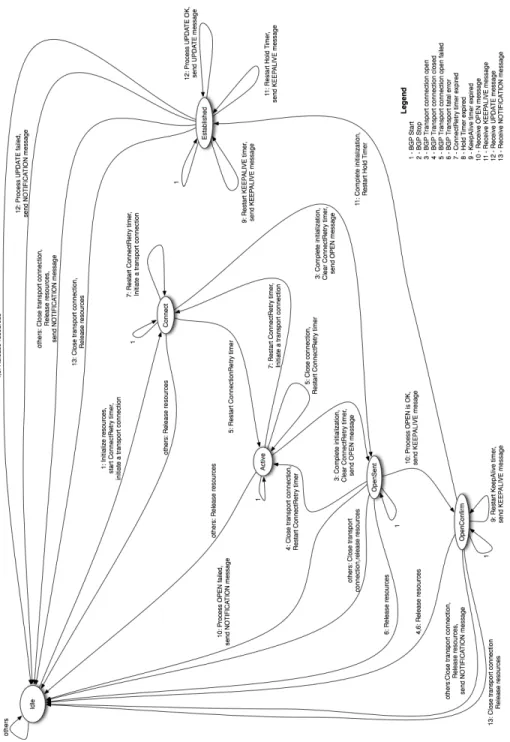
When two BGP peers connect they can exchange four different types of mes-sages to each other: open, update, keepalive, and notification. However, for a connection to first be established, a Transmission Control Protocol (TCP) con-nection must be made between the two BGP peers. With a TCP concon-nection the two routers can then exchange BGP open messages to create a BGP connection between them. The complete connection-making process is described by a Finite State Machine (FSM) as defined in RFC 1771 [63], and is shown in Figure 2.1. Once the connection is established, the two systems can exchange other BGP messages and routing information.
Figure 2.1: The Border Gateway Protocol connection Finite State Ma-chine.
This thesis focuses primarily upon the connectionist perspective of BGP net-works. However, for more information on the routing table and the various attributes associated with BGP paths, see Cisco’s Internetworking Technology Handbook BGP Documentation [22].
2.2.1
BGP Monitoring Tools
This section will first assess the current BGP monitoring tools available, fol-lowed by various network monitoring tools that utilize some form of machine learning for the detection of failures or faults within a network.
In terms of BGP network monitoring tools, each of the most recent tools as listed in the incredibly verbose survey [24] will be briefly assessed. Of the four listed tools, the first is BGPlay [23], which is a Java application that displays animated graphs of routing activity within a specified time interval. Next is BGPMon [75], which can monitor routes and alert in case of an ‘interesting’ path change. Path changing became a high-interest topic when YouTube was taken offline due to false path broadcast [54]. The next tool of interest is iBGPlay [8], which is a free tool that, similar to BGPlay, graphically displays and animates BGP routing data and thereby enables a user the ability to timely identify and diagnose potential routing problems and anomalies. Lastly, LinkRank [44] offers a different approach in visualization by creating graphs that weigh the links between autonomous systems by the number of routing paths going through each link. However, out of all four tools, none contain a machine-learning mechanism.
2.2.2
Network Monitoring Tools Utilizing Machine
Learn-ing
The following is a brief survey of tools and techniques that monitor a network utilizing some form of machine learning.
The first technique is dynamic syslog mining for network failure monitoring, as presented in [85]. In this work, the authors pursue network failure correlation and detection through monitoring syslogs. A syslog is a sequence of events which are collected using the BSD syslog protocol and are used to address a wide range of important issues including network failure symptom detection and event cor-relation discovery. The authors propose a new methodology of dynamic syslog mining in order to detect failure symptoms with higher confidence, to discover sequential alarm patterns among computer devices, and to detect event correla-tions among syslogs for different devices. As stated by the authors, the key ideas of dynamic syslog mining are 1) to represent syslog behavior using a mixture of Hidden Markov Models, 2) to adaptively learn the model using an on-line dis-counting learning algorithm in combination with dynamic selection of the optimal number of mixture components, and 3) to give anomaly scores using universal test statistics with a dynamically optimized threshold. Strictly with respect to machine learning techniques, a mixture of a hybrid Baum-Welch algorithm for learning Hidden Markov Models and a Naive Bayes model to learn patterns were utilized within the syslog data. The validity of this technique has been demon-strated through the use of real syslog data in the scenarios of failure symptom detection, emerging pattern identification, and dynamic correlation discovery.
Another technique is predicting node availability in peer-to-peer networks, as presented in [55]. In this work the authors improve upon the accuracy of
previous peer-to-peer availability models, which are often too conservative to dynamically predict system availability at a fine-grained level. Three types of availability predictors are utilized: 1) A graph-based representation to represent likelihood of traversal, 2) linear prediction (a common statistical technique for predicting time series), and 3) hierarchical accuracy tournaments to dynamically select the most accurate sub-predictor for a particular lookahead interval. Here, the machine learning techniques used are saturating counter predictors and a linear predictor which are trained via availability traces. Though this technique does not consider fault detection, network administrators often need notification of availabilities just as much as for failures.
An additional technique is manifold learning visualization of network traffic data, as presented in [61]. In this work, the authors present a manifold learning-based tool for the visualization of large sets of data and allows for an easy com-parison of data maps over time. This tool emphasizes the unusually small or large correlations that exist within a given data set along with an online Java-based GUI which allows interactive demonstration of the use of the visualization method. Moreover, data collection for visualization is made possible through the use of sensors which are located through a network that measure a chosen traffic statistic and divide traffic by source or destination IP address, port, autonomous system, time period, link, or router. Furthermore, this technique mainly consid-ers monitoring a network for changes over time, across space (at various routconsid-ers in the network), over source and destination ports, IP addresses, or AS numbers. Another technique is detecting anomalies in network traffic using maximum entropy estimation, as proposed in [33]. In this technique, the authors develop a behavior-based anomaly detection method that detects network anomalies by comparing the current network traffic against a baseline distribution. The
maxi-mum entropy learning technique provides a flexible and fast approach to estimate the baseline distribution, which also gives the network administrator a multi-dimensional view of the network traffic by classifying packets according to a set of attributes carried by a packet. By computing a measure related to the relative entropy of the network traffic under observation with respect to the baseline dis-tribution, this technique can distinguish anomalies that change the traffic either abruptly or slowly. Moreover, information is given regarding the type of anomaly detected and has a low false positive rate.
The next technique is an agent-based simulation of behavioral anticipation, specifically with regard to anticipatory fault managment in computer networks, as proposed in [67]. In this work, the authors explore the concept of anticipatory behavior to develop an intelligent agent-based network management model. An anticipatory agent is used to proactively detect occurrence of faults using a pre-dictive model pertaining to network performance. Prediction is possible through the machine learning technique of a Bayesian classifier trained with past data. The agent is therefore an entity which uses the knowledge of predicted future states to decide what actions need to be taken at the present.
Another technique is anomaly detection by finding feature distribution out-liers, as proposed in [71]. Here, the authors develop a means to detect traf-fic anomalies based on network flow behavior. First, baseline distributions for meaningful traffic features are estimated and measures of legitimate correspond-ing deviations are taken. Observed network behavior is then compared to the baseline behavior by means of a symmetrized version of the Kullback-Leibler di-vergence. The achieved dimension reduction enables effective outlier detection to flag deviations from the legitimate behavior with high precision. The actual machine learning mechanism is the application of probability mass functions in
conjunction with Kullback-Leibler divergence for learning the baseline network function. This technique supports online training and provides enough infor-mation to efficiently classify observed anomalies and allows in-depth analysis on demand.
The next technique involves exploring event correlation for failure prediction, as shown in [30]. In this work, the authors develop a spherical covariance model with an adjustable timescale parameter to quantify the temporal correlation and a stochastic model to describe spatial correlation. This is accomplished through the use of failure signatures, which extract the essential characteristics from a system state that are associated with a failure event and consider the hierarchical structure and interactions among components of the system. The authors further utilize the information of application allocation to discover more correlations among failure instances. Failure events are clustered based on their correlations and then used to predict similar future occurrences. The actual tool implemented is a failure prediction framework, called PREdictor of Failure Events Correlated Temporal-Spatially (hPREFECTs, where the ‘h’ stands for hierarchical), which explores correlations among failures and forecasts the time-between-failure of future instances, making use of both a neural network approach and a Bayesian network to learn and forecast failure dynamics based on the temporal and spatial data among the failure signatures.
An additional technique is an adaptive distributed mechanism used against flooding network attacks, as introduced in [9]. Here, the authors focus on early detection and the stop of distributed flooding attacks and network abuses. The framework cooperatively detects and reacts to abnormal behaviors before the target machine collapses and network performance degrades. In this framework, nodes in an intermediate network share information about their local traffic
ob-servations, improving their global traffic perspective. Also, the authors add to each node the ability of learning independently with a Naive Bayesian method to classify different types of traffic, therefore allowing each node to react differently according to its situation in the network and local traffic conditions. The learn-ing component also allows the system to create, adjust, and renew the behavior models. This then frees the administrator from having to guess and manually set the parameters distinguishing attacks from non-attacks; now such thresholds are learned and set from experience or past data.
Another technique involves detecting attack signatures in the real network traffic with ANNIDA (Artificial Neural Network for Intrusion Detection Appli-cation) which is discussed in both [69] and [26]. In these works, a Hamming Net artificial neural network methodology was used with good results where strings in computer network packets are inserted in these neural networks for pattern classification. Test results highlight the high accuracy and efficiency of the appli-cation when submitted to real data from HTTP network traffic containing actual traces of attacks and legitimate data.
Another technique utilizes a cascading neural network (CNN) for traffic man-agement of computer networks, as shown in [19]. In this work, the machine learning component consists of a two-level neural network model where one level (the back-propagation neural model), detects whether the tested network is over-loaded and the second level, a counter-propagation neural model, classifies and excludes the status of congestion derived from the overload of tested network. In this way, if the effect gained from the first level neural model is positive, the second level neural model will be triggered to help reroute the traffic of computer networks. To validate this two-level neural network feasibility, the proposed CNN has been applied to a local area network environment. The experimental results
demonstrate that the developed CNN can efficiently and effectively provide sub-stantial assistance for decision making in network traffic management.
Chapter 3
Domain Details
This chapter will discuss, in further detail, the two domains of interest for this thesis: BGP and neural networks.
3.1
BGP and SNMP
The primary work in this thesis is focused on the rigorously defined connection protocol for two BGP peers to start a session (as shown in the previous chapter), rather than the functionality of BGP in exchanging and storing routing informa-tion. Additionally, the focus of this work is oriented around network management of a single AS of interest, such as the domain that an administrator would have control over changing. Thus, the focus of this thesis is placed on iBGP rather then eBGP since only the network health of a single AS is of concern.
To provide some idea of the number of BGP Speakers in large Internet Service Provider (ISP) networks, see Table 3.1. These numbers will allow for designing representative experiments for scalability purposes in terms of the number of
ASN ISP Name Total Routers BGP Speakers
7018 AT&T 731 46
1239 Sprint 497 56
701 WorldCom/UUNet 4556 235
2914 Verio 865 80
3561 Cable & Wireless 2236 238
3356 Level3 483 61
6461 AboveNet 247 39
3967 Exodus 213 32
Table 3.1: BGP Speaker numbers for representative Internet Service Providers Backbones, as shown in [48].
BGP Speakers in Chapter 5.
One additional detail regarding iBGP is the moderately recent addition of route-reflection (RR), as shown in RFC 2796 [6] and RFC 4456 [7]. Route-reflection serves as an alternative to a fully-meshed iBGP network in that it can drastically reduce the number of required TCP sessions between BGP peers. A fully-meshed set of N BGP speakers must have N(N2−1) unique TCP Sessions, which presents obvious scalability issues when only 40 nodes yields 780 TCP sessions.
The best way to describe how route-reflection works is by example, as dis-cussed in [6]. Given a simple three-node network as shown in Figure 3.1, both Figure 3.1a and Figure 3.1b represent the same three-node BGP network within the same AS and all links are iBGP sessions. In the case of Figure 3.1a, when RTR-A receives an external route that is selected as the best path, it must then advertise that path to both RTR-B and RTR-C. Once received, RTR-B and
(a) Full mesh iBGP (b) Route reflection iBGP
Figure 3.1: Full Mesh vs. Route Reflection iBGP.
RTR-C will not re-advertise this path. However, in the case of Figure 3.1b, when RTR-A receives the same route, it would then advertise only to RTR-C. In the case of route reflection, RTR-C is now allowed to re-advertise (or reflect) the path learned from RTR-A to RTR-B and vice versa. This shows that the need for the additional iBGP session between RTR-A and RTR-C is unnecessary. Thus, the option of route reflection seems appropriate for large-scale networks and a representative topology will be assessed during experimentation.
Lastly, the particular monitoring methodology will be via the Simple Network Management Protocol (SNMP). As stated in [72], “SNMP enables network ad-ministrators to manage network performance, find and solve network problems, and plan for network growth”. Moreover, SNMP is a fairly common methodology for network and BGP monitoring [37], and fits well into the scope of this thesis.
3.2
Neural Network Architecture
3.2.1
Biological Inspiration
The name “neural” network makes a direct connection to that of biological neural structures. Such a connection is very appropriate since the concept of mathematical and computation neural networks were inspired and designed, in part, thanks to the connectionist theories of the brain. For this reason, a brief overview of biological neurons will be considered and translated into the mathe-matical model that is used in this thesis.
First of all, the typical structure of a biological neuron is shown inFigure 3.2. For the purpose of computational neural networks, the key features of the neuron are the dendrites, the axon/axon terminal, and the cell body. In a biological neural network, the dendrites collect neurotransmitters from the axon terminals of adjacent neurons, as shown inFigure 3.3. These signals are accumulated within the cell body and, if a certain level have been ascertained, the neuron will also fire, sending its own signal out through its axon [58]. These high-level functions are translated directly into the mathematical model of a neuron.
Figure 3.3: Two connected biological neurons [31].
To explain the translation from the biological neuron to a computational model, consider Figure 3.4. As shown in 3.4a and 3.4b, the dendrites on the biological neuron are represented by the inputs and synapses of the mathematical model, the cell body is the neuron core, and the axon retains the name axon but is simply the output of the mathematical neuron.
(a) Biological Neuron [60] (b) Mathematical Model [32]
Figure 3.4: The biological neuron and mathematical counterpart.
The internals of the computational neuron’s core contains two things: a sum-mation transfer function which feeds into an activation function. A closer look
at these features can be seen in Figure 3.5. With regard to activation functions, several types are permissible, ranging from a simple step function to a hyper-bolic tangent with output typically constrained within [0, 1] or [-1, 1]. Some representative activation functions are shown in Figure 3.6. And finally, when many mathematical neurons are connected together in layers, a resulting artificial neural network forms, as shown in Figure 3.7.
Figure 3.5: Details on the mathematical neuron core [83].
3.2.2
The Backpropagation Learning Algorithm
As noted in the previous chapter, the backpropagation algorithm was first introduced in 1974 [79] yet is still highly applicable today. All neural networks implemented in this thesis will be trained via this algorithm. The mathematical learning function associated with this algorithm will be described visually followed by a high-level perspective on how this learning technique can be utilized in a simple problem.
Since the purpose of this thesis is to propose a novel utilization of the well-established neural network backpropagation learning algorithm rather than to modify or enhance the learning algorithm itself, the algorithm’s mathematical details will not be assessed in rigor. Rather, for an in-depth exposition on the backpropagation algorithm, see [64]. However, to summarize, the backpropaga-tion learning algorithm is designed for a multi-layered feedforward neural network, as shown in Figure 3.7.
Figure 3.7: This is a standard multi-layered feedforward neural net-work, as shown in [21].
To train a neural network, the end-goal of training would be to have the network map a set of training inputs (input to the first layer of the neural network) where each individual input has a desired corresponding output value (outputs
on the last layer of the neural network). So, given a multi-layered feed-forward neural network such as the one shown in Figure 3.7, along with a set of inputs and corresponding set of outputs, the backpropagation algorithm trains the neural network on the input/output set so that it learns to map each of the inputs with the desired result. This is accomplished through modifying the weights on each of the synapses that inter-connect the neurons. These weights scale the input to a given neuron, which thereby modifies the output from a neuron’s axon. Typically, the weights on a neural network start out randomized, meaning that for each input string the output will be some unmeaningful string since the network has not yet been trained. Therefore, before the backpropagation algorithm runs, an error term can be calculated for each input based upon the current output for that value as compared with the desired output. This (desired result - actual result) error term is precisely what the backpropagation algorithm minimizes–thereby reducing the error discrepancy between the real output and desired output of the current neural network. This feedback loop is shown visually inFigure 3.8.
Figure 3.8: The training loop for a neural network, as shown in [21]. In this case the Training Algorithm is the backpropagation algorithm.
The backpropagation algorithm is also iterative–running a variable number of times, where each iteration is a step closer to the global minimum [21]. Also,
since the error term is slowly being minimized during each training iteration of the backpropagation algorithm, the training error can be visualized as a multi-dimensional error-surface, shown in Figure 3.9, where the current state of the neural network error is shown to be the dot on the error surface. Thus, as this figure shows, the end goal of training would be to reach the global minimum on the error surface, which corresponds to the point at which all the desired inputs map as closely as possible to the appropriate outputs. Furthermore, there are two specific parameters that can be fine-tuned on the backpropagation algorithm: learning rate and momentum. The learning rate parameter essentially represents the ‘speed’ of the virtual point on the error surface, basically specifying the step-size of the point for each iteration. Momentum, on the other hand, represents the ‘inertia’ of the point meaning that the degree of change to the weight of a given edge in the neural network during one training iteration impacts the change to that weight during the next iteration.
Figure 3.9: An example of a three-dimensional error surface for a training neural network, as shown in [52].
One potential problem while training neural networks is the potential for over-training or over-fitting. Over-training occurs when a network has learned
not only the basic mapping associated with input and output data, but also the subtle nuances and even the errors specific to the training set. If too much training occurs, the network essentially only memorizes the training set and loses its ability to generalize to new data input. The result is a network that performs well on the training set but performs poorly on out-of-sample test data.
One exemplary visual example for the utilization of neural networks would be for filling in the blanks on a mathematical function. Consider Figure 3.10. In this example, the graphed training data as shown in Figure 3.10a would be used by a simple neural network to generate the corresponding neural network output as shown in Figure 3.10b. Though a very simple example, this illustrates an inherently beneficial property of neural networks to “fill-in” the blanks between the training data points.
(a) Graphical training data (b) Trained neural network output
3.2.3
Architectural Design Decisions
In deciding on which type of neural network architecture to implement, a traditional feedforward approach was favored rather than recurrent neural net-works, since recurrent neural networks face inherent disadvantages as stated by Alessandro Sperduti:
...it is well known that training recurrent networks faces severe problems (Bengio, Simard, and Frasconi, 1994) and the generaliza-tion ability might be considerably worse compared to standard feed-forward networks (Hammer, 2001). [70]
Moreover, several studies have evaluated the computing capacity of multi-layered feed-forward neural networks [51, 68, 76, 80, 81, 82]. One such study found that
Feed-forward networks with a single hidden layer and trained by least-squares are statistically consistent estimators of arbitrary square-integrable regression functions under certain practically-satisfiable as-sumptions regarding sampling, target noise, number of hidden units, size of weights, and form of hidden-unit activation function. [80]
Essentially, such results have proven that multi-layered feed-forward neural networks with a single hidden layer are capable of approximating any real-valued function to any desired degree of precision.
The primary neural network architecture to be utilized in this thesis is a three-layered feed-forward neural network: one input layer, one hidden layer, and one output layer. However, two neural network versions will be utilized, both of which are shown in Figure 3.11. The neural network shown in Figure 3.11a is defined to be a General neural network, whereas the neural network shown in Figure 3.11b is defined as an Expert neural network. These two architectures
are nearly identical and differ only in the number of output nodes in the output layer. For the purposes of this thesis, the value of output nodes on the neural net-works correspond to the predicted health state of a corresponding router. Thus, these two architectures differ only in the number of routers they are responsible for. Additional details on the specific utilization of these architectures will be discussed in the next chapter.
(a) A General neural network
(b) An Expert neural network
Chapter 4
Design and Implementation
This chapter will go over the high-level conceptual design for constructing a BGP Failure detection and prediction tool as well as the specific details of the software implementation.
4.1
High-Level Concept Design
This section will discuss interfacing a iBGP network with a neural network, followed by the approach utilized in collecting training data.
4.1.1
Utilizing Neural Networks
The objectives of the design are to interface a generic iBGP network with a neural network, train the neural network with relevant past data, and then utilize the trained neural network along with the current iBGP connection statuses to make predictions and detections regarding the health of the BGP nodes. In order to assist the explanation, consider the visualization of a simple iBGP network as
shown in Figure 4.1. Shown in the figure is the iBGP network of interest in AS 4 and R1-R5 represent BGP routers 1 through 5 in a full mesh of connectivity.
Figure 4.1: An example of a simple BGP network.
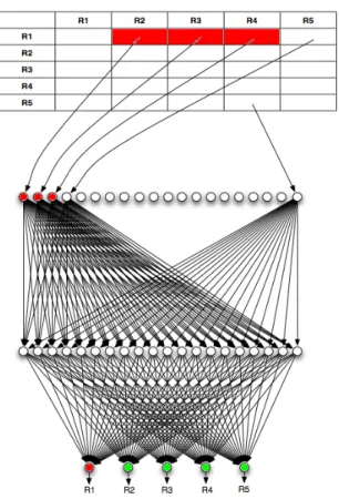
In preparation to interface the iBGP network to a neural network, an adja-cency matrix is utilized to represent each of the edge connections in the full mesh, as shown in Figure 4.2. In the adjacency matrix, the connection from R2 to R5 (as an arbitrary example), would be found by locating the cell whose column is R2 and whose row is R5. Moreover, in the case of this particular matrix, each entry contains a BGP finite state machine that stores the current state of the corresponding connection from one router to another. In this way, each of the six states associated with representing a peer-to-peer connection can be assigned a numeric value between 0 and 1 representing the degree of connectedness for the given session. With numbers assigned to each potential state, these values can then be the inputs to a neural network, as shown in Figure 4.3a. In this case, the neural network is defined to be a General neural network, since it is responsible for outputing the belief states of all nodes in the iBGP network. An alternative to this approach would be to interface the adjacency matrix with five
unique Expert neural networks, as shown inFigure 4.3b.
Figure 4.2: Interfacing the iBGP network with an adjacency matrix.
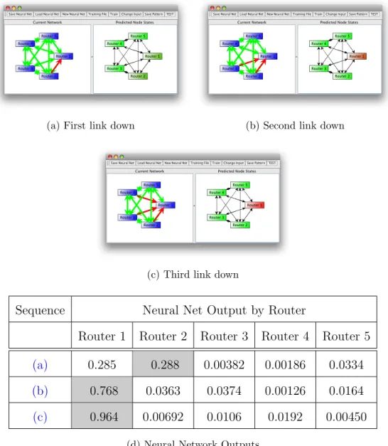
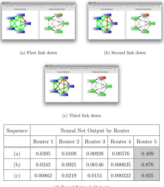
Now, consider the following simple example of how this high-level design should function end-to-end. For this example, the same iBGP network will be utilized with the modification that Router 1 loses connection with three of its neighbors, as shown in Figure 4.4. These lost connections can be followed down into the adjacency matrix and then into the neural network as shown inFigure 4.5. In this example, the neural network sees that even though Router 1 has not lost connection with all of its neighbors, a prediction is made that it is about to go down since the majority of connections has been lost while the other four routers are predicted to remain online. This example, of course, is under the assumption that a similar event has transpired in the past, training data had
(a) Interfacing the iBGP adjacency ma-trix with a General Neural Network
(b) Interfacing the iBGP adjacency ma-trix with an Expert Neural Network
Figure 4.3: Interfacing the adjacency matrix to a neural network.
been collected from the event, and the General neural network had been trained with the relevant data.
4.1.2
Training Data Collection Methodology
Though the methodology for collecting training data is not the focal point of this thesis, the design details are important nonetheless. The end goal in ascertaining representative training data would be to select a connectivity pattern from the network prior to a node being detected as going offline. Thus, the first requirement would be to detect whenever a node goes down.
For the purposes of this work, BGP peer failure is defined to be the case where a given BGP speaker loses connection with other speakers. This is considered
Figure 4.4: Router 1 loses connection to three of its neighbors.
Figure 4.5: The resulting adjacency matrix and neural network output from Router 1 losing three connections.
a failure due to the fact that if a BGP speaker loses connection to its peers, then routing information cannot be transmitted–the BGP peer has failed its job and purpose. More specifically, two types of node-down failure patterns will be considered. First, an “externally-detected-node-down” (EDND) will refer to the case when, given node N, all nodes in the network have lost connection to N. In this case, all routers in the network would be incapable of updating the EDND router’s routing table. On the other hand, a “self-detected-node-down” (SDND) will refer to the case when a given node N is found to have lost connection to all nodes it was previously connected to. In this case, the SDND router would be incapable of updating any other peers in the network. Therefore, some pre-processing must be executed to generate both of these possible node-down signatures and stored for reference when monitoring the corresponding network. With the capability of detecting a node-down established, the next require-ment would be to maintain a pattern history list for the network. An addition would be made to this list (or queue) every time there is some session state change within the network. In this way, all patterns leading up to a node failure would be stored for later access as training data. However, this brings to light the fi-nal requirement: a way to specify where excactly in the queue history to look for appropriate training data. Thus, some particular lookbackvariable must be defined such that when a node-down is detected, the pattern located within the history queue at a distance of lookback will be saved as a pre-cursor predic-tion pattern for the given node-failure. And lastly, this solupredic-tion is appropriate for a single node going offline, but there may be multiple correlated nodes that go down as well, say in the case that two routers are on the same power grid during a black-out. In this special case, a different distance specifier may be de-sired, so acorrelatedLookback variable should also exist and be independently
configurable from the standardlookback variable.
4.2
Software Implementation Details
The Java software written for this thesis is dubbed the BGP Neural Network Framework (BGPNNF). Moreover, note that this software is not designed with the intention of use as a polished tool for a network administrator. Rather, the framework software implementation presented in this section has been designed and written for experimental purposes to prove the hypothesis of this thesis, namely: Neural networks can interface with iBGP computer networks to learn and utilize the precursor connectivity patterns that emerge prior to a node failure. To present the BGPNNF, this section will present the relevant configuration options, the backend programmatic details, and some simple user interface details.
4.2.1
The User Interface
The BGPNNF user interface (UI) is designed solely to assist in the experi-ments for this thesis and provide a visual representation of the neural network inputs and outputs. Therefore, the UI is rather minimal and basic, as shown in Figure 4.6. The interface was implemented using the org.jdesktop.application-.Application and org.jdesktop.application.Action libraries and utilizes JGraph [3] and JGraphT [59] for the graph visualizations. Lastly, line charts are generated through the use of JFreeChart [49].
The major features of the interface are the row of buttons across the top of the main window, along with two network views. The network views are the most important feature of the user interface–the one on the left displays the
Figure 4.6: The BGPNNF User Interface.
current network connection states (which are the inputs to the internal neural network) whereas the view on the right side are the predicted node states (the output from the neural network(s)). An example of these views in action are shown in Figure 4.7. As shown, the red connections in the Current Network view show the links that are down or Idle and the corresponding Predicted Node States view shows which node is predicted to have issues. In terms of coloring, all inputs/outputs of the neural network are contained within the range [0.0, 1.0]. Thus, as for color displays ranging between green (good) and red (bad) for some given state and defining 1 to represent disconnected (0 represents established), the color displays are therefore simplyColor(state, 1 - state, 0), where the three parameters are red, green, and blue, respectively.
With regard to the row of buttons, each one has a specific function relevant to experimentation. Each button will be described in terms of functionality, moving from left to right.
Figure 4.7: Example distinguishing the current view from predicted. In this case, Router 4 has lost the majority of its connections and is therefore predicted to go completely offline by the red coloring in the prediction panel.
question is the netChooser button. This button allows the user to select which Expert neural network will be affected by any of the other buttons shown. As such, this button only appears if a backend Expert neural network implementa-tion is being run.
The next button is the “Save Neural Net” button. This button, as its name implies, serializes the current backend neural network to a file. Upon clicking this button, a standard JFileChooser dialog is displayed to choose the location and file name to save the neural network, as shown in Figure 4.8. This feature is of particular value when, after training a neural network for experimental purposes, it can be stored and returned to at another time. Thus, complementary to the Save button comes the next “Load Neural Net” button. This button functions much like the Save button in that, upon clicking, a JFileChooser dialog is opened, which allows the user to navigate to the previously saved neural network and
Figure 4.8: Save Dialog User Interface.
restore it, as shown inFigure 4.9.
Figure 4.9: Load Dialog User Interface.
Continuing sequentially, the following button is the “New Neural Net” button. This button removes the internal neural network and replaces it with a newly specified neural network. When clicked, this button opens a dialog to specify how many nodes are to be located in the hidden layer (the input and output layers are fixed), as shown in Figure 4.10.
Figure 4.10: New Neural Net User Interface.
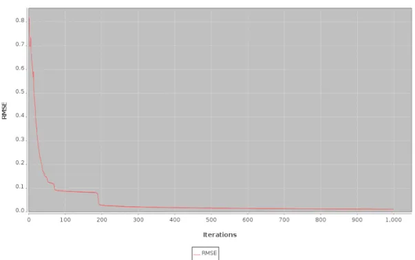
The next button on the user interface is titled “Training File”. When clicked, this button opens a JFileChoose dialog that allows the user to navigate to the directory and file that contains the training data desired for training the internal neural network. The next button “Train” utilizes the training file to train the internal neural network. When clicked, the Train button opens a dialog as shown inFigure 4.11. As shown in the figure, the training parameters of Learning Rate, Momentum, and number of Iterations must be specified prior to training. Also, a lower-bound can be set for the resulting Root Mean Squared Error (RMSE) of the neural network through the “Desired RMSE” setting which will halt training if the RMSE of the network drops below the specified value. This feature helps to ensure that the neural networks do not become over-trained. Moreover, an additional check-box is available in this panel to optionally graph the RMSE versus iterations of the training.
The remaining three buttons are present strictly for testing and debugging purposes. The “Change Input” button stops and starts the internal SNMP polling mechanism. The “Save Pattern” button allows the current state of the neural network to be saved to the current training file. Lastly, the “TEST” button simply runs an internal test method for debugging purposes.
Figure 4.11: Train Button User Interface.
entitled the “Input Test Network Display”, as shown in Figure 4.12. This UI allows a user to manipulate the individual session states between the displayed routers. As shown, a radio button can be selected as either “down” or “up”, corresponding to the session state to be set as either up (established connection) or down (idle connection). Once the radio button has been set to the desired value, the user then clicks one router (session origin) followed by clicking a second router (session destination). The directed session between the two machines is then set to the value of the positioned radio button. This feature will allow for various combinations of testing to be performed separate from when the software is directly connected with and polling the hardware routers.
4.2.2
Relevant Configuration Options
The configuration utility of the BGPNNF parses an XML file that speci-fies the network topology, neural network type, number of nodes in the neural network hidden layer, and the size and lookback options for the historyQueue
Figure 4.12: The input test network user interface.
of pattern changes in the network. The XML parser of the BPGNNF utilizes javax.xml.parsers.Document-Builder, javax.xml.parsers.DocumentBuilderFactory, along with org.w3c.dom.Document, org.w3c.dom.Element, org.w3c.dom.Node, and org.w3c.dom.NodeList. In order to elaborate upon the configuration op-tions specifiable within the configuration file, example XML code in conjunction with visuals will be presented.
By far, the most important configuration option for the BGPNNF is specifying the network topology of interest. In order to specify a topology, a list of nodes (routers) must be defined in terms of name and interface IPs with corresponding lists of adjacent IPs. The resulting design to meet these requirements is shown in Code Block 4.1. In this case, the router name is simply Router 1 and contains two different interfaces with IPs 208.94.60.1 and 208.94.60.15. Within each interface tag are adjacent tags, which represent which peer IPs can be reached from each interface. Thus, 208.94.60.1 has one adjacent peer, namely 208.94.60.2, whereas interface 208.94.60.15 has two peers: 208.94.60.16 and 208.94.60.20. In order
to actually specify a complete network topology, however, many nodes must be defined. One example is shown in Code Block 4.2, which specifies the simple five-node fully-connected network as shown in Figure 4.13.
1 <node name="Router 1"> 2 <interface IP="208.94.60.1"> 3 <adjacent IP="208.94.60.2" /> 4 </interface> 5 <interface IP="208.94.60.15"> 6 <adjacent IP="208.94.60.16" /> 7 <adjacent IP="208.94.60.20" /> 8 </interface> 9 </node>
Code Block 4.1: Example Node XML Element and Contents
With the network topology specified, the next most important configuration option is the type of neural network architecture to use and interface with the defined network topology. For the purposes of this thesis, the type of neural network must be specified as either a General neural network or an Expert neural network within the XML neuralNet element. An example of a General neural network configuration is shown in Code Block 4.3. As shown in the example, to choose a General neural network theexpert attribute of theneuralNet element must be set to false. Moreover, since the neural network contains a hidden layer, the number of nodes in that layer must be specified with thehiddenNodeselement
Figure 4.13: A simple fully-connected five-node network, as specified by Code Block 4.2.
and the number of nodes set to the num attribute. Lastly, the training data for the neural network is stored within an external text file, so the external file is specified within the trainingData element under the file attribute. In this example, the training file is simply set to “trainingData.txt”.
On the other hand, an Expert neural network configuration is shown inCode Block 4.4. In the Expert case, the expert attribute is now set to true, but the biggest differentiating characteristic from the General neural network con-1 <node name="Router 1"> 2 <interface IP="208.94.60.1"> 3 <adjacent IP="208.94.60.2" /> 4 <adjacent IP="208.94.60.3" /> 5 <adjacent IP="208.94.60.4" /> 6 <adjacent IP="208.94.60.5" /> 7 </interface> 8 </node> 9 <node name="Router 2"> 10 <interface IP="208.94.60.2"> 11 <adjacent IP="208.94.60.1" /> 12 <adjacent IP="208.94.60.3" /> 13 <adjacent IP="208.94.60.4" /> 14 <adjacent IP="208.94.60.5" /> 15 </interface> 16 </node> 17 <node name="Router 3"> 18 <interface IP="208.94.60.3"> 19 <adjacent IP="208.94.60.1" /> 20 <adjacent IP="208.94.60.2" /> 21 <adjacent IP="208.94.60.4" /> 22 <adjacent IP="208.94.60.5" /> 23 </interface> 24 </node> 25 <node name="Router 4"> 26 <interface IP="208.94.60.4"> 27 <adjacent IP="208.94.60.1" /> 28 <adjacent IP="208.94.60.2" /> 29 <adjacent IP="208.94.60.3" /> 30 <adjacent IP="208.94.60.5" /> 31 </interface> 32 </node> 33 <node name="Router 5"> 34 <interface IP="208.94.60.5"> 35 <adjacent IP="208.94.60.1" /> 36 <adjacent IP="208.94.60.2" /> 37 <adjacent IP="208.94.60.3" /> 38 <adjacent IP="208.94.60.4" /> 39 </interface> 40 </node>
figuration is the specification of training data files. In the General case, only one training file was specified since there is only a single neural network. In the case of the Experts, alternatively, since there is one expert per node in the network, there must be one training file per node. The trainingData element is utilized once again, but the router element is now utilized to specify which training file correponds to which router, therefore assigning the file to the neural network responsible for the given router. For example, in the case of the first
trainingData element, the neural network responsible for Router 1 would use the expertData1.txt training file.
1 <neuralNet expert="false">
2 <hiddenNodes num="12" />
3 <trainingData file="trainingData.txt" />
4 </neuralNet>
Code Block 4.3: Example neuralNet Element for Configuring a General Neural Network
1 <neuralNet expert="true">
2 <hiddenNodes num="20" />
3 <trainingData router="Router 1" file="expertData1.txt" />
4 <trainingData router="Router 2" file="expertData2.txt" />
5 <trainingData router="Router 3" file="expertData3.txt" />
6 <trainingData router="Router 4" file="expertData4.txt" />
7 <trainingData router="Router 5" file="expertData5.txt" />
8 </neuralNet>
Code Block 4.4: Example neuralNet Element for Configuring an Ex-pert Neural Network
The last configuration options of interest are the settings associated with the historyQueue. A sample configuration is shown in Code Block 4.5. The three configurable settings are as follows: 1) the size of the queue (essentially the length of the sliding-window of retained history), 2) the length of lookback
nodes down. As shown in the example, the size of the queue is set using the
size attribute in the historyQueue element. The second configuration is the lookback number, which, when a node-down is detected, specifies how far back in the queue to look for the pre-cursor pattern to use as training data for the neural network. Again, as shown in the example, this is specified by setting the
lookback attribute in the historyQueue element. Lastly, when multiple nodes go down, a different lookback history may be desired, which can be specified by setting the correlatedLookback attribute, which is set to 4 in the example. 1 <historyQueue size="10" lookback="2" correlatedLookback="4"/>
Code Block 4.5: Example Configuration of the historyQueue
4.2.3
Backend Programmatic Details
The primary points of interest for the backend implementation consist of initi-ating the SNMP polling mechanism, creiniti-ating the signature strings for detecting a node-down, initializing thehistoryQueue, constructing the neural network from the configuration file, and instantiating the CoreModel. The descriptions will follow in line with the high-level flow diagram as shown in Figure 4.14.
Creating the SNMP Poller
The SNMP Poller modual utilizes the Java SNMP4j [28] library to sequen-tially poll each router, as specified in the configuration file. So, the only required information is a list of nodes to poll and this is accomplished through a list of custom NodeInfo objects. The primary components of a NodeInfo object are shown in Code Block 4.6. As shown in the code, the String name
repre-Figure 4.14: The BGPNNF Flow Diagram.
sents the name of the router. The String[] interfaceIPs represent the list of interfaces, ie ethernet ports, by IP on the named router. Lastly, each of the String IP addresses located within the interfaceIPs array serve as a key in the
HashMap<String,String[]> adjacentmap, and the corresponding value is an-otherStringarray comprised of all the external IPs that this router is connected to.
1 private String name;
2 private String[] interfaceIPs;
3 private HashMap<String, String[]> adjacent;
Code Block 4.6: NodeInfo Private Variables.
Once theNodeInfolist is built, then polling can commence when the “ChangeIn-put” button on the UI is clicked. Polling is conducted as shown in Code Block
4.7.
1 private boolean poll; //boolean value for continuous polling
2 while(poll)
3 {
4 for (int i = 0; i < nodes.length; i++)
5 {
6 String[] interfaceIPs = nodes[i].getInterfaceIPs();
7 for (int j = 0; j < interfaceIPs.length; j++) {
8
9 String[] adjacentIPs = nodes[i].getInterfaces().get(interfaceIPs[j]);
10 for (int k = 0; k < adjacentIPs.length; k++) {
11
12 nodeState = pinger.snmpGet(interfaceIPs[j], bgpSNMP.READ_COMMUNITY,
13 bgpSNMP.OID_BGP_PEER_STATE + adjacentIPs[k]);
14
15 //update the CoreModel
16 //’6’ corresponds to Established
17 if (nodeState.equals("6")) {
18 model.update(interfaceIPs[j], adjacentIPs[k], 0);
19 }
20 //If not established, then the session is considered down
21 else { 22 model.update(interfaceIPs[j], adjacentIPs[k], 1); 23 } 24 } 25 } 26 } 27 }
Code Block 4.7: SNMP Poller Main Loop.
Creating the Node-Down Detection Signature Strings
Creating the node-down detection signature strings is the last pre-processing that takes place prior to the start of SNMP polling. This requires only the
NodeInfo array and every possible EDND and SDND pattern is recorded into the nodeDownPatternList private variable of the CoreModel, as shown in Code Block 4.8. These signatures are then utilized during each update if the matrix
has changed. If there is a change, the nodeDownCheck() method is called, which is shown in Code Block 4.9. Note that the goal of nodeDownCheck() is to de-termine if the current matrix pattern is a subset of any of the strings in the
spite of other noise in the network.
History Queue
The private OQueue historyQueue of the CoreModel is a fairly standard queue that maintains a finite interval of history, as specified in the configuration file. In addition
![Figure 3.9: An example of a three-dimensional error surface for a training neural network, as shown in [52].](https://thumb-us.123doks.com/thumbv2/123dok_us/761621.2596412/39.918.269.669.652.897/figure-example-dimensional-error-surface-training-neural-network.webp)