OpenAIR@RGU
The Open Access Institutional Repository
at Robert Gordon University
http://openair.rgu.ac.uk
Citation Details
Citation for the version of the work held in ‘OpenAIR@RGU’: AL MOUBAYED, N., 2014. Multi-objective particle swarm optimisation: methods and applications. Available from
OpenAIR@RGU. [online]. Available from: http://openair.rgu.ac.uk
Copyright
Items in ‘OpenAIR@RGU’, Robert Gordon University Open Access Institutional Repository, are protected by copyright and intellectual property law. If you believe that any material
Optimisation: Methods and
Applications
Noura Al Moubayed
A Thesis submitted in partial fulfilment of the requirements of the
Robert Gordon University for the degree of Doctor of Philosophy
Solving real life optimisation problems is a challenging engineering ven-ture. Since the early days of research on optimisation it was realised that many problems do not simply have one optimisation objective. This led to the development of multi-objective optimizers that try to look at the optimisation problem from different points of view and reach a set of com-promised solutions among the different objectives. The presented research brings together recent advances in the field of multi-objective optimisation and particle swarm optimisation raising several challenges. This is tackled from different aspects including the proposal of new archiving techniques to developing new methods and quality measures. Smart Multi-objective Particle Swarm Optimisation based on Decomposition (SDMOPSO) is first proposed to incorporate multi-objective problem decomposition techniques with PSO. A novel archiving technique is developed using a clustering based mapping approach between the objective and solution spaces and is applied
to general multi-objective optimizers. D2M OP SO is introduced as a new
MOPSO that uses problem decomposition and a new archive utilising dom-inance based mapping between objective and solution spaces. Finally the thesis presents a novel multi-objective quality measure that uses mutual information to compare among solutions generated by different algorithms. The contributions are all tested on standard test suits and are used to solve two real-life problems: a) Channel selection for Brain-Computer Interfaces, and b) Effective cancer chemotherapy treatments. The two problems are real challenges in the two respective fields. Two different modelling ap-proaches of the channel selection problem are presented: one is based on binary representation of the channels, while the other is continuous in a projected space of the channel locations. The results are very competitive with the commonly used methods.
• N. Al Moubayed, A. Petrovski and J. McCall, D 2 MOPSO: Multi-Objective Particle Swarm Optimizer Based on Decomposition and Dominance, Evolutionary Computation, MIT Press.
• N. Al Moubayed, A. Petrovski and J. McCall, Mutual information for
perfor-mance assessment of multi objective optimisers: Preliminary results, The 14th International Conference on Intelligent Data Engineering and Automated Learn-ing (IDEAL’2013).
• N. Al Moubayed, A. Petrovski and J. McCall, D 2 MOPSO: Multi-Objective
Particle Swarm Optimizer Based on Decomposition and Dominance, Evolution-ary Computation in Combinatorial Optimization (EvoCop 2012) Volume 7245 of Lecture Notes in Computer Science, Springer Berlin / Heidelberg, pp 75-86.
• N. Al Moubayed, B. Awwad Shiekh Hasan, J. Q. Gan, A. Petrovski and J.
Mc-Call, Continuous Presentation for Multi-Objective Channel Selection in Brain Computer Interfaces, proceedings of the World Congress on Computational In-telligence, WCCI 2012, Brisbane, Australia, IEEE.
• N. Al Moubayed, A. Petrovski and J. McCall, Clustering-Based Leaders
Selec-tion in Multi-Objective Particle Swarm OptimisaSelec-tion, Intelligent Data Engineer-ing and Automated LearnEngineer-ing (IDEAL 2011), Volume 6936 of Lecture Notes in Computer Science, Springer Berlin / Heidelberg, pp. 100-107.
• N. Al Moubayed, A. Petrovski and J. McCall, Clustering based Framework for
Leaders Selection in Multi-Objective Evolutionary Algorithms, Proceedings of the 13th annual conference on genetic and evolutionary computation (GECCO 2011), Dublin, Ireland, ACM, pp. 96-96.
Symposium on Computational Intelligence in Multicriteria Decision-Making in conjunction with IEEE Symposium Series on Computational Intelligence (SSCI 2011), April 2011, Paris, France, IEEE.
• N. Al Moubayed, A. Petrovski and J. McCall, A Novel Smart Multi-Objective
Particle Swarm Optimisation using Decomposition, In Parallel Problem Solving from Nature (PPSN XI), 2010, volume 6239 of Lecture Notes in Computer Sci-ence, Springer Berlin / Heidelberg, pp. 1-10.
• N. Al Moubayed, B. Awwad Shiekh Hasan , J. Q. Gan, A. Petrovski and J.
McCall, Binary-SDMOPSO and its Application in Channel Selection for Brain-Computer Interfaces, In 10th Annual Workshop on Computational Intelligence (UKCI 2010), September 2010, Colchester, UK, IEEE.
I would like to thank my PhD advisors, Doctor Andrei Petrovski and Pro-fessor John McCall, for supporting me during these past four years. Andrei was always supportive and has given me the freedom to take decisions and follow my research interests. He has always given me his invaluable advice and opinion. Without his support and encouragement I would not have achieved what I have achieved and I definitely would not be able to publish as much. John is a very sweet person, his kindness will make you instantly love him and never forget him. He is very smart, funny, friendly and has a real Scottish spirit. I enjoyed every single discussion and learnt from his great experience.
I will forever be thankful to my beloved husband who was and still is a true and great supporter. Bashar, thank you for standing by me, being positive at all times and most of all thanks for being patient with my, sometimes, irritable mood and stubbornness, and giving me all the love and care in the world. I love you loads and all the words in the world cannot express my appreciation. you are the meaning of my life and with you I am not afraid of anything, The outcome of my PhD is not only a thesis and some papers but also an awesome baby girl. Julie, you made my life bright and beautiful, you are my sunshine. I cannot be anything but happy and excited when you are around.
I especially thank my mom, dad, and brothers. they have never stopped supporting me for a second. They put their faith in me and gave me all the support in the world. Dad and mum, you are great parents and I would not imagine my life without you both. Samer, thank you for your support, advice and funny jokes, thanks for being so loving and caring. Hsnee, my
I thank my lovely dog, Lassie, who kept my feet warm while writing up and accompanied me in my walks and breaks. Lassie you are a piece of my heart.
I dedicate this thesis to my family, my husband, Bashar, my beautiful baby, Julie and my dog, Lassie for their great support and love. I love you all from all of my heart.
Abstract i
List of Publications ii
Acknowledgment ii
List of Figures ix
List of Tables xiv
1 Introduction 1
1.1 Motivation . . . 2
1.2 Aims and Objectives . . . 3
1.3 Methodology . . . 4
1.4 Summary of Contributions . . . 5
1.5 Thesis Outline and Organization . . . 6
2 Literature Review 7 2.1 Introduction . . . 8
2.2 Single Objective Optimisation . . . 8
2.3 Population-based Metaheuristics . . . 10
2.3.1 Initial Population . . . 10
2.3.2 Generation . . . 11
2.3.3 Selection . . . 11
2.3.4 Stopping Criteria . . . 11
2.4 Particle Swarm Optimisation . . . 12
2.4.2 Theoretical analyses and Convergence . . . 18
2.5 Multi-objective Optimisation . . . 20
2.6 Multi-objective Evolutionary Algorithms . . . 23
2.6.1 Algorithms based on Aggregation Functions . . . 23
2.6.2 Non-dominated Sorting Genetic Algorithm (NSGA) and NSGAII 25 2.6.3 Multi-objective Evolutionary Algorithms based on Decomposi-tion (MOEA/D) . . . 25
2.7 Multi-Objective Particle Swarm Optimisation . . . 27
2.8 Archiving in MOPSO . . . 29
2.8.1 Leaders in MOPSO . . . 29
2.8.2 Archiving and Spreading of Nondominated Solutions . . . 30
2.8.2.1 Kernel: . . . 31
2.8.2.2 Adaptive Grid Algorithm . . . 31
2.8.2.3 Niche Count . . . 31
2.8.2.4 Clustering . . . 32
2.8.2.5 −dominance . . . 32
2.8.2.6 Nearest Neighbour Density Estimator . . . 33
2.8.3 Diversification and Avoidance of Local Optima . . . 35
2.8.3.1 Position Update . . . 35
2.8.3.2 Turbulence . . . 36
2.9 Multi-objective PSO algorithms . . . 37
2.9.1 Aggregating Approaches . . . 37
2.9.2 Pareto-based Approaches . . . 38
2.9.3 Combined Approaches . . . 41
2.9.4 Decomposition-based Approaches . . . 42
2.9.5 Convergence Properties of MOPSO . . . 43
2.10 Quality Measures . . . 44
2.10.1 Error Ratio . . . 46
2.10.2 Generational Distance . . . 46
2.10.3 Inverted Generational Distance . . . 46
2.10.4 Hypervolume . . . 47
2.10.5 Indicator . . . 47
3 Methods 50
3.1 Introduction . . . 51
3.2 SDMOPSO . . . 51
3.2.1 The Algorithm . . . 52
3.2.2 Why SDMOPSO? . . . 54
3.2.3 Experiments and results . . . 55
3.2.4 Discussion . . . 56
3.3 Clustering based Framework for Leaders Selection . . . 60
3.3.1 Principal Component Analysis . . . 62
3.3.2 Density Based Spatial Clustering . . . 62
3.3.3 The Algorithm . . . 64
3.3.4 Experiments and Results . . . 67
3.3.5 Discussion . . . 73
3.4 D2M OP SO: MOPSO based on Decomposition and Dominance . . . 74
3.4.1 Archiving based on Crowding Distance in Objective and Solution Spaces . . . 75
3.4.2 The algorithm . . . 77
3.4.3 Novelty of D2M OP SO . . . 82
3.4.4 Selected Test Problem . . . 82
3.4.5 Experimental Setup . . . 83
3.4.6 Performance Metrics . . . 84
3.4.7 Results and Discussion . . . 87
3.4.8 Numeric Comparison . . . 87
3.4.9 Visual Comparison . . . 90
3.4.10 Analysis of Computational Complexity . . . 91
3.4.11 Discussion . . . 92
3.5 Conclusion . . . 93
4 Applications 106 4.1 Introduction . . . 107
4.2 Channel Selection for Brain-Computer Interfaces . . . 108
4.2.1 Modeling Multi-Objective Channel Selection Problem . . . 109
4.2.3 Experiments and Results . . . 111
4.2.3.1 Data Set . . . 111
4.2.3.2 Feature Extraction and Classification . . . 111
4.2.4 Continuous Presentation for Multi-Objective Channel Selection in Brain-Computer Interfaces . . . 117
4.2.5 Experiments and Results . . . 119
4.2.5.1 Sequential Forward Floating Search . . . 119
4.2.5.2 Data Recording and Pre-processing . . . 120
4.2.5.3 Feature Extraction and Classification . . . 121
4.2.5.4 D2M OP SO parameter settings . . . 121
4.2.6 Results . . . 121
4.3 Finding Effective Cancer Chemotherapeutic Treatments: . . . 125
4.3.1 Cancer Chemotherapy . . . 126
4.3.1.1 Medical Aspects of Chemotherapy . . . 126
4.3.1.2 Problem Formulation . . . 127
4.3.2 Customized-SDMOPSO for Cancer Chemotherapy Treatment . . 130
4.3.3 Experiments and Results . . . 131
4.4 Conclusion and Discussion . . . 138
5 Mutual Information for Performance Assessment of Multi Objective Optimisers 142 5.1 Introduction . . . 143
5.2 Measuring Quality of Multi-objective Optimizers . . . 144
5.3 Methods . . . 146
5.3.1 Mutual Information . . . 146
5.3.2 Measuring Quality with Mutual Information . . . 147
5.3.3 Processing Pareto Fronts as Images . . . 148
5.3.4 Handling Outliers: . . . 150
5.4 Experiments . . . 151
5.4.1 Selected Test Problem . . . 151
5.4.2 Experimental Setup . . . 151
5.5 Results and Discussion . . . 152
6 Conclusions 159
6.1 Summary of Contributions . . . 160
6.2 Future Work: . . . 162
6.3 In Conclusion ... . . 163
2.1 Diagram of an empty topology. A circle represents a particle and the
directed arrow represents a direct link indicates a self connection. . . 16
2.2 Diagram of a local best topology. A circle represents a particle and the
directed arrow represents a direct link indicates a self connection, while
the non-directed link represents a two-way link between two particles. . 16
2.3 Diagram of a global best topology. A circle represents a particle and the
directed arrow represents a direct link indicates a self connection, while
the non-directed link represents a two-way link between two particles. . 16
2.4 Diagram of a start topology. A circle represents a particle and the
di-rected arrow represents a direct link indicates a self connection, while
the non-directed link represents a two-way link between two particles. . 17
2.5 Diagram of a tree topology. A circle represents a particle and the directed
arrow represents a direct link indicates a self connection, while the
non-directed link represents a two-way link between two particles. . . 17
2.6 A chart diagram of the general PSO algorithm. . . 19
2.7 An example of a multi-objective optimisation problem: A) the
parti-cles/solutions in the search space B) the corresponding Pareto front. . . 22
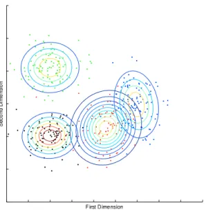
2.8 Example of the result of a clustering algorithm (Gaussian Mixture Model). 33
2.9 To the left, the area dominated, in a minimization problem, by a certain
solution is highlighted. To the right the area being dominated has been
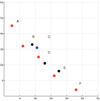
2.10 −dominance in two dimensional objective space. The red dots are the selected particles. In box B the black particle is removed as it is domi-nated by the red one. In box D the red and the black particles are not comparable, i.e. no one dominates the other, so the red particle is chosen as it is more to the left. Box C is discarded because it is dominated by
B and D. . . 34
2.11 Example of nearest neighbour density estimator in two dimensional space. 35 2.12 An example of Sigma-MOPSO. . . 39
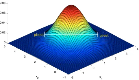
2.13 Illustration of the Gaussian distribution used by dMOPSO for generating a new particle. The personal best and the global best are used to define the mean and variance of the Gaussian distribution. . . 43
3.1 (a, e, i) are the P Ftrue and the rest are the approximated ones . . . 57
3.2 (a, d) are P Ftrue and the rest are the approximated ones . . . 58
3.3 Example of clusters produced by Density Based Spatial Clustering . . . 64
3.4 Example of the algorithm at work while mapping clusters. . . 65
3.5 The two PF approximations for ZDT1. . . 69
3.6 The two PF approximations for ZDT2. . . 69
3.7 The two PF approximations for ZDT3. . . 69
3.8 The two PF approximations for ZDT4. . . 70
3.9 The two PF approximations for ZDT6. . . 70
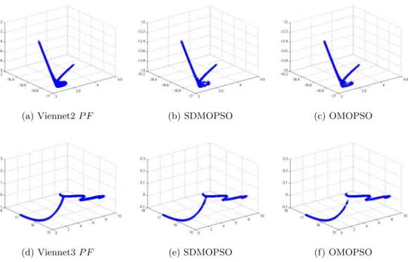
3.10 The two PF approximations for Viennet2. . . 70
3.11 The two PF approximations for Viennet3. . . 71
3.12 Box plots to demonstrate the average distance between each solution of the actual Pareto front and its closest solution in the approximated PF. NSGAII results are at the left of each sub plot, while NSGAII/C results are at the right side. . . 72
3.13 Coverage set results for the two algorithms. For each problem 2 bars are drawn, the left bar represent the percentage of solutions produced by NSGAII that dominate these produced by NSGAII/C, the right bar represents the opposite percentage. . . 72
3.14 Dominance-based ranking for the non-dominated solutions of the leaders’ archive using the crowding distance values in both solution and objective spaces. X-axis is the crowding distance in the solution space, Y-axis is the crowding distance in the objective space. The numbers next to each particle represents its rank. In this example the particles ranked with 3
are the best. . . 76
3.15 Swarm of 20 particles in a sample objective space. When only decompo-sition is used 8 particles are directed to promising regions in the space, the remaining 12 are directed to unpromising ones, i.e. 60% of the swarm is wasting the search effort. . . 78
3.16 Plot of the non-dominated solutions with the lowest IGD values in 30 runs ofD2M OP SO, MOEA/D and OMOPSO for solving Viennet4. . . 84
3.17 Plot of the non-dominated solutions with the lowest IGD values in 30 runs ofD2M OP SO. . . 86
3.18 Plot of the non-dominated solutions with the lowest IGD values in 30 runs ofM OEA/D. . . 87
3.19 Plot of the non-dominated solutions with the lowest IGD values in 30 runs ofdM OP SO. . . 88
3.20 Plot of the non-dominated solutions with the lowest IGD values in 30 runs ofOM OP SO. . . 89
3.21 The evaluation of IGD for the four algorithms. . . 94
3.22 The evaluation of Hyper Volume for the four algorithms. . . 95
3.23 The evaluation of the four algorithms for Viennet4. . . 102
4.1 Solutions obtained by OMOPSO. The approximated Pareto front related to every subject is marked by the corresponding letter. . . 112
4.2 Solutions obtained by MOEA/D. The approximated Pareto front related to every subject is marked by the corresponding letter. . . 114
4.3 Solutions obtained by Binary-SDMOPSO. The approximated Pareto front related to every subject is marked by the corresponding letter. . . 115
4.4 Box plot of the accuracies achieved using the three methods. The average accuracy using each of the method is also shown. . . 116
4.5 Box plot of the number of selected channels achieved using the three methods. The average number of selected channels using each of the
method is also shown. . . 116
4.6 Projected Biosemi 64+2 EEG channel locations. The numbering scheme follows the standard Biosemi numbering. Inclusion circles are drawn around each channel. . . 118
4.7 The structure of the synchronous trials . . . 120
4.8 Frequency of Channels selected via SFFS . . . 122
4.9 Results using D2M OP SO. Results of each subject are plotted with a polynominal fit of degree 2 to show the approximated Pareto Front. . . 123
4.10 Comparison between accuracy results obtained using SFFS andD2M OP SO124 4.11 Frequency of Channels selected via D2M OP SO. . . 125
4.12 Approximated Pareto fronts . . . 134
4.13 The reference set obtained by merging all the non-dominated solutions generated by the three algorithms . . . 134
4.14 Box plot of the IGD achieved using the three methods (the central line in every box represents the median; the average IGD using each of the algorithms is shown as a numeric value) . . . 135
4.15 Drug doses for one of MOEA/D solutions . . . 137
4.16 Drug doses for one of NSGA-II solutions . . . 137
4.17 Drug doses for one of c-SDMOPSO solutions . . . 138
5.1 An example of two unequal PFs with the same histogram. The blue PF (A) is the true PF for ZDT1 and the red PF (B) is a shifted copy of the blue PF.IM I(A,A) = IM I(A,B) = 1. . . 148
5.2 The blue dots belong to a hypothetical true PF. The red dots belong to a hypothetical approximated PF. The dots within the circle belong to the approximated PF and are considered outliers. . . 150
5.3 Results of ZDT1 using three algorithm: NSGAII,SPEAII, and IBEA compared using four indicators: IIGD,I,Ihv, and IiM I. . . 153
5.4 Results of ZDT2 using three algorithm: NSGAII,SPEAII, and IBEA compared using four indicators: IIGD,I,Ihv, and IiM I. . . 154
5.5 Results of ZDT3 using three algorithm: NSGAII,SPEAII, and IBEA
compared using four indicators: IIGD,I,Ihv, and IiM I. . . 155
5.6 Results of ZDT4 using three algorithm: NSGAII,SPEAII, and IBEA
compared using four indicators: IIGD,I,Ihv, and IiM I. . . 156
5.7 Results of ZDT6 using three algorithm: NSGAII,SPEAII, and IBEA
2.1 A comparison among commonly used problems: F1 is the number of objectives. F2 is the geometry of the Pareto Front. F3 does the problem
have any bias (+) or not (-). F4 the number of constraints. . . 49
3.1 Indicators values for the three methods applied on nine test problems: the values are presented as [GD,R-metrics] . . . 58
3.2 Inverted Generational Distance results for the two algorithms . . . 71
3.3 Average Generational Distance results for the two algorithms . . . 73
3.4 A comparison among the decomposition-based MOEA under study . . . 84
3.5 A comparison of computational complexity . . . 92
3.6 Results ofIIGD on unconstrained bi-objective test problems . . . 96
3.7 Results ofIhv on unconstrained bi-objective test problems . . . 97
3.8 Results ofI on unconstrained bi-objective test problems . . . 98
3.9 Results ofIIGD on unconstrained three-objective test problems . . . 99
3.10 Results ofIhv on unconstrained three-objective test problems . . . 100
3.11 Results ofI on unconstrained three-objective test problems . . . 101
3.12 Results ofIIGD on constrained test problems . . . 102
3.13 Results ofIhv on constrained test problems . . . 103
3.14 Results ofI on Constrained test problems . . . 104
3.15 Main Features of the Performance Measures . . . 104
4.1 RESULTS USING OMOPSO . . . 113
4.2 RESULTS USING MOEA/D . . . 114
4.3 RESULTS USING Binary-SDMOPSO . . . 115
4.5 Maximum Results usingD2MOPSO . . . . 124
4.6 The side-effects of the drugs used through the treatment . . . 132
4.7 Drug profiles of the anti-cancer agents used . . . 133
4.8 Inverted Average Generational Distance results for the three algorithms 135
4.9 Cardinality measure results for the three algorithms . . . 136
5.1 Values of the quality indicators with and without outliers in the
approx-imated PF. . . 151
5.2 Statistical significance of the difference between theIIGD values for the
different algorithms applied on the 5 problems. A 4means the method
indicated by the column is significantly better than that indicated by
the raw, i.e. p < 0.05. / mean the raw is significantly better than the
column. - means there is no significant difference, i.e. p > 0.05. The
problems are ordered as follows: ZDT1-ZDT4,ZDT6 . . . 156
5.3 Statistical significance of the difference between the I values for the
different algorithms applied on the 5 problems. A 4means the method
indicated by the column is significantly better than that indicated by
the raw, i.e. p < 0.05. / mean the raw is significantly better than the
column. - means there is no significant difference, i.e. p > 0.05. The
problems are ordered as follows: ZDT1-ZDT4,ZDT6 . . . 157
5.4 Statistical significance of the difference between the Ihv values for the
different algorithms applied on the 8 problems. A 4means the method
indicated by the column is significantly better than that indicated by
the raw, i.e. p < 0.05. / mean the raw is significantly better than the
column. - means there is no significant difference, i.e. p > 0.05. The
problems are ordered as follows: ZDT1-ZDT4,ZDT6. . . 158
5.5 Statistical significance of the difference between theIiM I values for the
different algorithms applied on the 8 problems. A 4means the method
indicated by the column is significantly better than that indicated by
the raw, i.e. p < 0.05. / mean the raw is significantly better than the
column. - means there is no significant difference, i.e. p > 0.05. The
Introduction
“Human beings, viewed as behaving systems, are quite simple. The apparent complexity of our behavior over time is largely a reflection of the complexity of the environment in which we find ourselves.”
1.1
Motivation
In the late 1980s, Eshel Ben-Jacob began to study the self-organization of bacteria in
the hope of understanding more complex biological systems. He developed new
pattern-forming bacteria species,Paenibacillus vortex andPaenibacillus dendritiformis.
P. dendritiformis revealed an intriguing collective ability, which is viewed as a
pre-cursor of collaborative intelligence, the ability to switch between different morphotypes
to better adapt with the environment (Ben-Jacob(2003)). Scientists have only recently
started to understand, how bacteria can quickly adapt to changes in the environment, distribute tasks, learn from experience, prepare for the future and make decisions. Bac-teria in a colony, numbering many times the population on Earth, exchange chemical messages to synchronize their behavior.
Ants were first characterized by entomologist W. M. Wheeleras cells of a single
superorganism . What appears to be independent individuals can actually work so
closely as to become indistinguishable from a single organism (Wheeler(1912)). Later
research regarded some insect colonies as examples of collective intelligence. The
con-cept of ant colony optimization algorithms, introduced by Marco Dorigo, became
a popular theory of evolutionary computation. Colonies allocate workers to different tasks, and workers switch from one task to another in response to changing conditions.
Kennedy & Eberhart(1995) studied the collective behaviour of a flock of birds and showed that they manifest a collective intelligence behaviour in the environment. His simulation of the bird flocks led to a family of optimisation algorithms that can be collectively called: Particle Swarm Optimization (PSO).
Collective intelligence in principle assumes the individuals are simple in nature but the interaction among the individuals yields sophisticated behavior. This principle is exploited in order to solve complex optimisation problems by making the individuals navigate the search space of the problem in order to cover the surface of the function to be optimized. This simple but revolutionary idea lead to great advances in optimisation and metaheuristics with applications in many fields of science and engineering.
However, many real-life applications are far more complicated than the assumption that there is one ultimate goal of the optimisation process. Some problems can have several competing goals, so that getting closer to one goal may lead the individuals further away from the other goals. To tackle these problems a compromise must be
reached among all the goals of the optimisation process. This has shown to be a real challenge to the optimization community.
The motivation of this research is to look at PSO from a multi-objective perspec-tive, i.e. modify the original PSO method so that it can handle complex problems with conflicted optimisation goals. The thesis builds on the state-of-the-art of both PSO and multi-objective optimisation and contributes to both fields on different levels and through the different stages of the optimisation process. As the real judge of an optimizer is its applicability in the real world, the thesis applies the newly developed methods on real-life applications showing the potential of these methods and their impact.
1.2
Aims and Objectives
The main goal of the thesis is to enrich the discipline of multi-objective optimisation with a set of new techniques to tackle challenging problems in the extension of PSO to the multi-objective domain. These new techniques will cover the main steps in a multi-objective PSO from neighbourhood definition of the particles to archiving and quality testing. The thesis builds on recent development in multi-objective optimisation which uses decomposition with genetic algorithms as the way to break down the multi-objective problem into simpler single multi-objective ones and then solve these problems simultaneously. Decomposition is incorporated in the two main algorithms presented
(SDMOPSO andD2M OP SO), in addition to a new concept for archiving which creates
a mapping between objective and solution spaces.
The secondary aim of the thesis is to test the developed techniques on real-life prob-lems. To this end two problems were solved using the new algorithms: 1) The channel selection in Brain-Computer Interfaces 2) The dose regulation in Cancer chemotherapy. The thesis presents several solutions to these two problems in terms of problem design and results interpretation. The work on these two problems was in close collaboration with experts in the respected fields to ensure the quality of the data analysis.
The third, and final, objective of the thesis is to develop a new quality assessment measure for multi-objective optimisers. For the first time, the thesis presents a novel measure that uses mutual information as the basis for an indicator that sees the Pareto
fronts as images and applies mutual information to measure the quality of the approxi-mated PF given the true one. This novel approach is much robust against outliers than the other commonly used measures as demonstrated in the thesis.
It should be stressed that although the thesis uses PSO as the basic optimiser, the developed techniques are general and can be used by other evolutionary optimisers
(e.g. GA) as demonstrated in Section3.3where the new archive is applied on NSGAII
instead of PSO.
1.3
Methodology
The research carried out in this thesis followed a strict procedure to guarantee high quality results and robust conclusions. This is demonstrated by my publications in high impact journals and conferences. The procedure consists of the following steps:
• problem identification: identify interesting research questions to answer and study
the possibility of making significant contribution to address these questions.
• development: a solution(s) of the problem is considered and algorithms and
meth-ods are developed to tackle the problem in hand. The newly developed methmeth-ods are tentatively tested in order to get feedback and adjust the methods accordingly.
• experimental design: to thoroughly test the developed methods experiments are
run using standard problems. The results are compared to those of the state-of-the-art and based on the outcome of the comparison going back to development might be necessary.
• publication: the results are written and submitted to appropriate medium of
publication in order to get feedback from the community to enhance the work. The first identified problem was the definition of particles’ neighbourhood within multi-objective PSO. The state-of-the-art MOPSO used techniques borrowed from the single objective PSO. I , on the other hand, have incorporated the decomposition ap-proach into PSO in order to redefine the neighbourhood in PSO to better solve multi-objective problems. This work resulted in the development of Smart Multi-Objective PSO based on Decomposition (SDMOPSO).
Secondly the issue of archiving the generated solutions was tackled. The commonly used archives rely only on information in the objective space alone without into consid-eration the information in the solution space. Hence, I developed two solutions to map
the two spaces and building an archive based on either clustering or−dominance. This
lead to Clustering based framework for Leaders Selection (CLS), and later the develop-ment of a new MOPSO algorithm: MOPSO based on Decomposition and Dominance
(D2MOPSO).
The last theoretical identified challenge was the assessment of multi-objective opti-mizers. I have introduced a novel measure based on mutual information which is robust towards outliers.
A major evaluation part of any newly developed approach is the choice of evaluation problems. All the newly developed methods and algorithms were tested on commonly used test suits for multiobjective problems and real-life problems.
1.4
Summary of Contributions
The thesis contains four main tracks:
1. Archiving: this is a very important part of any evolutionary algorithm. Maintain-ing the solutions found within the optimisation process, decidMaintain-ing which solutions to dismiss and how to select the current leaders are all very sensitive part of any optimization process especially in the multi-objective paradigm. The thesis pro-poses a novel approach of archiving that maps the search and objective spaces to enhance the output solutions and their diversity.
2. Algorithms: two distinct algorithms are proposed in the thesis, namely
SD-MOPSO and D2M OP SO. They both share the inclusion of the concept of
decomposition, but they differ in how to deploy this concept and integrate it within the framework of PSO.
3. Quality Measures: the thesis proposes a new quality measure of the Pareto Front, i.e. the solution set of the optimiser, in order to compare among different algo-rithms. The measure uses mutual information capable of circumventing a major drawback of most of the trendy measures by using not the distance calculation (Euclidean or otherwise), but statistical information instead.
4. Applications: The real test of an optimisation algorithm is by testing it on real-life problems. Since the beginning of the work, I have collaborate with the Brain-Computer Interfaces (BCI) group in the university of Essex and have applied my algorithms on some technical problems related to selecting the best channels of a BCI system for control. I have also tested part of my work on the problem of deciding the dose of chemotherapy treatment for patients in order to enhance their quality of life while on treatment.
1.5
Thesis Outline and Organization
Next chapter reviews the basic concepts behind Particle swarm optimisation and multi-objective optimisation leading to identifying the problems to be addressed in the
fol-lowing chapters. Chapter 3describes the developed methods in this thesis including a
new archiving technique and new algorithms for MOPSO. Chapter 4 applies some of
the methods developed on real-life problems, while Chapter5introduces novel quality
Literature Review
“Artificial Intelligence, IT’S HERE. ” -Business Week cover, July 9, 1984
2.1
Introduction
Intuitively, optimisation is the selection of the best element, with regard to some cri-teria, from a set of possible elements. In its simplest form, an optimisation problem is about finding the value that minimizes (or maximizes) a given function, i.e. objective
function,(Gershenfeld (1998)). Practically, the shape of the objective function is
un-known and the optimisation is usually restricted with constraints in the search space complicating the optimisation process.
Many optimisation methods have been developed over the years. Rothlauf (2011)
provided detailed taxonomy of optimisation methods and the principles of solving an optimisation problem. Here we focus only on a particular type of optimizers, namely evolutionary algorithms, which are usually seen as metaheuristics. Metaheuristics make few or no assumptions on the problem to be solved which does not guarantee finding the optimal solution(s) to the problem. However, this same property allows for solving complicated optimisation problems.
Many problems in science and engineering require the simultaneous optimisation of more than one objective simultaneously. The challenge of solving multi-objective prob-lems raises from the complexity of these probprob-lems and the difficulty of finding reasonable solutions for all objectives. It is usually the case that enhancing the performance in terms of one objective would result in the deterioration of the other objectives. The solutions generated by the optimizer are then trade-off solutions among the different
objectives (Coello Coello et al. (2007)).
Coello Coelloet al. (2007) argued that the use of evolutionary algorithms (EAs) to solve multi-objective problems is mainly motivated by their population-based nature. This allows the generation of optimal solutions (called Pareto optimal solution as will be discussed later) in a single run. In addition, some multi-objective problems can be very complicated to be solved by conventional deterministic optimizers.
2.2
Single Objective Optimisation
Historically single objective optimisation was first developed in order to solve problems where there is only one goal to optimise. Most, if not all, evolutionary algorithms started by a single objective version and then some where extended to account for the multiobjective case.
A minimisation/maximization single objective optimisation problem is defined as
the minimization/maximization of a function f(x) : Ω ⊆ Rn → R,Ω 6= ∅ subject
to gi(x) ≤ 0, i = {1, . . . , m}, and hj(x) = 0, j = {1, . . . , p}, x = (x1, . . . , xn) ∈ Ω
(Coello Coello et al. (2007)).
gi(x)≤0 andhj(x) = 0 are constraints that must be fulfilled while optimizingf(x).
Ω contains all possiblex that can be used to evaluatef(x) and satisfy its constraints.
The method for finding the global optimum (minimum or maximum) which may not be unique is referred to as global optimisation.
For a minimization problem, the valuef∗ =f(x∗)>−∞is called a global minimum
(or global optima in general) if and only if
∀x∈Ω :f(x∗)≤f(x) (2.1)
x∗ is by definition the global minimum solution , f is the objective function, and
the set Ω is the feasible region ofx.
The shape of f(x) determines the difficulty of the optimisation problem. For a
relatively simple function exact optimisation can be sufficient (e.g. analytical and
numerical methods, Dynamic programming, etc... Rothlauf(2011)). In practice f(x)
can be much more difficult to optimize so heuristic based methods are needed (Rothlauf
(2011)), which in turn can cause the optimizer to fall in what is called a local optima.
The local optima is similar in definition to the global one,f∗, except that it is applied to
a smaller region of the search space. It is worth noting that local optima is not a unique
value forf(x) which could complicate the optimisation problem. Local optima can be
a problem for a lot of optimizers and especially the deterministic ones. Evolutionary algorithms may perform better to tackle this particular issue as they are stochastic in
nature and then may have better chance of getting out of a local optima (El-Ghazali
(2009)).
There is a comprehensive literature on single objective optimisation: numeric linear
algebra (Ciarlet(1989)), Dynamic programming (King(2002)), and many others. Here
we are only interested in a type of approximate optimizers namely the population-based
2.3
Population-based Metaheuristics
Population-based metaheuristics are stochastic optimizers and contain a considerable number of algorithms that are mostly inspired by nature, e.g. Evolutionary Algo-rithms (EAs), Particle Swarm Optimisation (PSO), estimation of distribution algo-rithms (EDAs) and many others. Despite their intrinsic differences these algoalgo-rithms share some common concepts:
• a population of potential solutions is initialized. The population and its members
are called differently in different algorithms.
• a new generation of the population is generated based on the experience of the
previous generation.
• the new generation is integrated with the old one using some selection criteria.
• this search process continues until a stopping condition is met, e.g. a pre-set
number of iterations is reached.
The implementation of these concepts varies significantly among different algo-rithms. Understanding how each of these steps is tuned and implemented is essential to get the best out of any population-based optimizer. These concepts are further discussed in some detail in the following sections.
2.3.1 Initial Population
By definition population-based metaheuristics are exploration search algorithms, i.e. the algorithm starts by exploring large areas of the search space and then narrows down the search throughout the optimisation process.
Maaranen et al. (2007) argued that the initialization step plays a crucial role in the effectiveness of the algorithm. When generating the initial solutions, the most important aspect is the diversity of these solutions. If the initial solutions are not diverse enough, i.e. do not cover large areas of the search space, they could lead the
algorithm to a premature convergence, i.e. falling into a local optima (El-Ghazali
(2009)).
Unlike other approaches, in the context of Evolutionary algorithms and PSO the
(2009)). The random generator is usually performed using pseudo-random numbers
utilising classical generators, e.g. recursive lagged Fibonacci, (Gentle(2003)).
2.3.2 Generation
In this phase, a new population is generated following the adopted generation strategy. There are mainly two generation strategies here:
• Evolutionary based: the solutions are selected and reproduced using a variation
operators (e.g. mutation) acting directly on the current population, so that the newly generated solutions are directly obtained from the variables representing
the solutions in the current population. Evolutionary algorithms and scatter
search are examples of such algorithms (El-Ghazali(2009)).
• Backboard based: In this approach the members of the population contribute to
a shared memory of the system. This share memory is then used to generate the new solutions. Particle swarm optimisation is an example of an algorithm that adopts this strategy. In PSO the best particle in the current population is considered the leader and affects the evolution of the solutions of the future particles in the swarm. The shared memory is then formed by this information
interaction among the particles in the swarm (Section2.4).
2.3.3 Selection
Once the new solutions are generated then the algorithm has to select the new popula-tion from the old populapopula-tion and the generated solupopula-tions. The simplistic method would be to use the generated solutions as the new population. Evolutionary algorithms usu-ally applies a selection mechanism where the best solutions of the two sets are selected to form the new population. In backboard-based heuristics there is not a direct selec-tion mechanism as the informaselec-tion exchange among the populaselec-tions’ members dictates the generation of the new population.
2.3.4 Stopping Criteria
Deciding on the stopping criteria is important as the algorithm should stop when it has converged on one side but it should not continue much after convergence is reached
as it causes wasting computational power. Stopping criteria can be static, i.e. the search ends when a fixed condition is satisfied, e.g. number of iterations, number of objective evaluations, etc. Alternatively an adaptive stopping criteria can be used such as a measure of objective approximation, or some statistics regarding the diversity of the reached solutions so far.
Next the Particle Swarm Optimisation is described in detail as it is the dominantly used algorithm in this work.
2.4
Particle Swarm Optimisation
Kennedy & Eberhart (1995) first proposed the idea of Particle Swarm Optimisation (PSO) as a method to attain computational intelligence based on the social interaction of individuals rather than the cognitive and intelligence competency of one individual. They established this type of intelligence by simulating the behavior of flocks of birds
or fish and then developed a powerful optimisation method, namely PSO, (Eberhart
et al. (1996);Kennedy & Eberhart (1995,1997a)).
In principle PSO distributes a set of entities, called particles, in the search space of an optimisation problem. Each of these particles evaluates the objective function at its current location. In order to determine its next step the particle combines its experience with the locations of the particles with the best fit, i.e. leaders, with some random perturbations. In one iteration all the particles are moved and then the swarm as a whole moves, as a flock of birds converging for food, hopefully towards an optimum value of the function. The first application to PSO was to tune the parameters of a
neural network (Eberhart et al. (1996)) but soon it gained popularity especially in
problems with continuous search spaces (Engelbrecht(2007)), despite a binary version
of the algorithm (Kennedy & Eberhart(1997a)).
Angeline(1998) andEberhart & Shi(1998) compared the mostly used evolutionary algorithms, genetic algorithms (GA) and PSO and two main distinctions can be made between the two:
1. Evolutionary algorithms rely on three main mechanisms: parent representation, selection of individuals, and the fine tuning of parameters. On the other side, PSO does not use an explicit selection mechanism but rather uses leader(s) to
guide the optimisation process. The offspring generation in PSO is different from GA in terms of using the backboard approach rather than the evolutionary one. 2. Another key difference between PSO and evolutionary algorithms is the way the particles are manipulated. PSO direct particles by manipulating their velocity and direction as a result using both the particle’s personal best and the global best (the leader’s). On the other hand EA uses mutation operators that can set the direction of the individual in any direction.
According toReyes-Sierra & Coello(2006) there are two main reasons for the
pop-ularity of PSO:
1. The PSO algorithm is relatively simple. The use of only one operator to create new solutions makes its implementation straightforward. In addition, there are plenty of reliable implementations online.
2. PSO is found to be very effective in many application domains producing com-petitive results at a low computational expense.
To solve a problem in a D dimensional search space using PSO, each particle is
composed of three D dimensional vectors: the current position −→xi, the previous best
position−−−→pbesti, and the velocity−→vi (Kennedy & Eberhart(1995);Poliet al.(2007)). −→xi
is designed to be a point in the search space. During optimisation the particle positions are evaluated after each iteration as solutions to the problem. If a new position is better
than what has been found so far, then it is stored in −−−→pbesti. The goal of the particle
within the optmisation is then to keep enhancing−−−→pbesti. The particle moves to a new
position in the search space by adding −→vi to −→xi. The algorithm adjusts −→vi which in
returns changes the direction and speed of the change in position.
By definition the particle alone can not solve the optimisation problem. It can only operate in collaboration with the other particles in the swarm. The interaction among the particles in the swarm is governed by the neighbourhood definition, usually referred to as topology or social network. Each particle communicates with the other particles in its neighbourhood and is affected by the best particle in this neighbourhood, denoted
Similar to other population-based metaheuristics PSO starts by randomly initializ-ing the particles in the swarm. The position of each particle is then changed accordinitializ-ing
to its own experience and that of its neighbours. The position of particlepi at time t
is changed by adding the velocity−→vi(t) to the current position:
− →x
i(t+ 1) =−→xi(t) +−→vi(t+ 1) (2.2)
The velocity vector reflects the socially exchanged information and is defined in the following way: − →v i(t+ 1) =W−→vi(t) +C1r1(−→xpbesti− − →x i(t+ 1)) +C2r2(→−xleader− −→xi(t+ 1)) (2.3)
wherer1, r2 ∈[0,1] are random values. leader refer to either the global leader or local
leader depending on the topology used. C1, C2 are learning factors, and W is the
inertia weight.
2.4.1 Parameters
PSO has a very few number of parameters to be set. The first parameter is the size of the population. This is usually set empirically and it would normally increase with the increase of dimensionality.
C1,C2 are called the learning factors or acceleration coefficients and represent the
magnitude of the particle in the direction of its personal best and its neighbourhood.
The values ofC1 and C2 can affect the optimization significantly as it can either make
the PSO more responsive to change or unstable. These parameters in short control the exploration exploitation balance of the algorithm and hence must be carefully chosen.
The inertia weight,W ∈[0,1], controls the influence of the previous velocity vectors
on the calculation of the current velocity. W is seen as a friction coefficient (Poliet al.
(2007)), and so can be considered as the fluidity of the medium in which a particle
moves. It might then be useful to start with a relatively highW (e.g. 0.9) which causes
the particles to behave in an explanatory mode, and then gradually reducing W to
around 0.4 where the system would be more exploitive. The strategy of updating W,
or not at all, is very important to the optimisation process. Eberhart & Shi (2000)
used a fuzzy system to adapt W. Zheng et al. (2003) showed that increasing inertia
Eberhart et al. (2001) showed that based on the network topology of the swarm, the movement of the particle can be greatly influenced by the neighbouring particles where the neighbourhood is defined by the swarm’s topology. Following are some of
the commonly used topologies (Engelbrecht(2007)).
• Empty Topology: here the particles are only driven by their experience, pbest,
which means that the particle is isolated from all the other particles. In this case
C2 is set to zero. Fig. 2.1shows an example of such a topology.
• Local best Topology: Each particle is directed by its neighbourhood. The
neigh-bourhood has a fixed size (n) and the movement of each particle is influenced by
the best performing particle in this neighbourhood. Fig. 2.2presents an example
of this network.
• Global best Topology: Also called fully connected topology. Each particle is
influenced by a global leader of the swarm, i.e. the particle with the best perfor-mance, in addition to its own experience. In order to achieve this each particle is
connected to every other particle in the swarm, Fig. 2.3.
• Star Topology: In this case only one particle,f ocal, is considered the head of the
swarm and all other particles are directly connected to it but are isolated from
each other. f ocal compares performance among all particles in the swarm and
adjusts its direction accordingly, Fig. 2.4.
• Tree Topology: All particles are arranged in a tree where each node of the tree
contains only one particle. Each particle is influenced by its own experience,
pbest, and that of the particle just above it in the tree. A child particle will
replace its parent if it had reached a better solution, Fig. 2.5.
There are other network topologies that can be used and these are well discussed in (Poli et al.(2007)).
Figure2.6illustrates the general PSO algorithm (single optimization). In line with
the population-based paradigm, PSO starts with an initialization step which includes
both velocities and positions. The correspondingpbestof each particle is also initialized
and the leader is identified (the leader definition depends on the network topology used). Then and for a maximum number of iterations the particles move in the search space
Figure 2.1: Diagram of an empty topology. A circle represents a particle and the directed arrow represents a direct link indicates a self connection.
Figure 2.2: Diagram of a local best topology. A circle represents a particle and the directed arrow represents a direct link indicates a self connection, while the non-directed link represents a two-way link between two particles.
Figure 2.3: Diagram of a global best topology. A circle represents a particle and the directed arrow represents a direct link indicates a self connection, while the non-directed link represents a two-way link between two particles.
Figure 2.4: Diagram of a start topology. A circle represents a particle and the directed arrow represents a direct link indicates a self connection, while the non-directed link represents a two-way link between two particles.
Figure 2.5: Diagram of a tree topology. A circle represents a particle and the directed arrow represents a direct link indicates a self connection, while the non-directed link represents a two-way link between two particles.
directed by their experience and the leader constrained by the network topology, the
particles then update their velocity, position, and pbest using Eq. 2.2, and Eq.2.3.
Finally the leader is updated and the iterations continue until the maximum number of iterations is reached.
2.4.2 Theoretical analyses and Convergence
Behind the apparently simplicity of PSO, it raises serious challenges for the theoretical understanding of its behaviour. Firstly, PSO consists of a large number of interacting particles. The particles themselves are simple to model but the interaction among these particles makes the modelling of such dynamic a complicated issue. Secondly, the particles has a memory which adds unpredictable factor to the modelling of the particles dynamics. This stochastic nature prevents the use of standard mathematical tools. Thirdly, the fitness functions can vary a lot and with them the behaviour of PSO.
For these reasons there is still no full mathematical modelling of PSO that captures
fully its behaviour, however there are some attempts to tackle this issue (e.g. Blackwell
(2007);Engelbrecht(2005);Kadirkamanathanet al.(2006)). Poliet al.(2007) provides a comprehensive review of these modelling attempts.
Engelbrecht(2005) showed that PSO is sensitive to the choice of control parameters. Most theoretical work on PSO made several simplification assumptions, the swarm is
usually considered consisting of one particle in a one dimensional space,pbestandgbest
are assumed constant throughout the process and so are φ1 = C1r1 and φ2 = C2r2.
Under these conditions the swarm convergence is defined as follows.
Definition 1 Giving the sequence of global best solutions {gbest}∞
t=0, the swarm is
converged iff: limt→∞gbestt=p
wherep is an arbitrary position in the search space.
Ozcan & Mohan(1998) studied PSO under the previous conditions without consid-ering the inertia weight. They showed that the trajectory of the particle can be seen as a sinusoidal wave where the initial conditions and parameter setting dictates the
amplitude and frequency giving that 0< φ <4 where φ=φ1+φ2.
Van Den Berghet al. (2002) built a similar model that accounts for inertia weight
Initialize Swarm
Locate Leader
iteration
<iterMax
iteration=0
Update Particles’ Positions
Evaluate Particles
Update
pbest
Update leader
iteration++
Stop
converges to φ1pbest+φ2gbest
φ1+φ2 . Then he generalized to the case where φ1 and φ2 are not
constant and he concluded that the swarm converges to (1−a)pbest+agbest where
a= C2
C1+C2.
Clerc & Kennedy (2002) presented an analytical analysis of PSO with constriction coefficients to prevent the velocity from growing out of bounds.
The analysis discussed so far prove, under certain assumptions, the convergence of PSO, but to ensure the convergence to the local or global optimum, two conditions
must be met: 1) monotonicity, i.e. gbestat a generationtcan not be worse than gbest
at the previous generation t−1. 2) the algorithm should generate a solution in the
neighbourhood of the optimum from any solution−→x in the search space.
Van Den Bergh et al. (2002) showed that PSO satisfies the first condition but not the second one so the original PSO can not be considered a global, or local, optimizer as there is no guarantee that it will reach a global/local optimum. The solutions suggested for this premature convergence problem of PSO include using mutation operators, or sub-swarms, or the reinitialisation of the swarm when the algorithm is converged. These simple solutions are usually effective enough for PSO to work in practice.
So far the algorithms and methods described are all interested in solving problems with a fitness function containing only one objective. Next section describes a more sophisticated type of problems: multi-objective optimisation problems, where more than one objective is involved in the optimisation problem complicating the job for the optimizer.
2.5
Multi-objective Optimisation
The traditional way of looking at optimisation problems as single objective, i.e. the fitness function is only concerned with one quantity to optimize, can lead in some real-life situations to sub-optimal solutions of the problem due to the misrepresentation of the optimisation problem. An alternative type of optimisation is described as multi-objective optimisation in which there are more than one multi-objective. These multi-objectives are usually conflicting in nature so any improvement in one objective often happens at the expense of deterioration in other objective(s). The optimisation challenge there-fore is to find the entire set of trade-off solutions that satisfy all conflicting objectives (Coello Coello et al. (2007)). Multi-objective optimization has roots in mathematical
optimization with the first multi-objective evolutionary algorithm (MOEA) presented
in 1985,Schaffer (1985). The field has grown rapidly in the last 10 to 15 years and is
now known a dominant area of research within the optimization community.
Coello Coello et al.(2007) presented a sophisticated description of the formal def-inition of multi-objective problems (MOPs). Here I use simplified defdef-initions that is
commonly used in the literature (Reyes-Sierra & Coello (2006)).
MOP is an optimization problem in the solution/search space Ω⊂Rn where an
n-dimensional vector−→x = [x1, x2, . . . , xn]T ∈Ω is defined and is referred to as the decision
variables vector. The problem’s objective is then defined as a vector of objectives in
the objective space: −→f(−→x)∈∆⊂Rm:
− →
f(−→x) = [f1(−→x), f2(−→x), . . . , fm(−→x)]T (2.4)
where m≥2 is the number of objectives, fi :Rn → R, i = 1, . . . , m are the objective
functions. For a minimization problem, without any loss of generality, the goal of the
optimizer is to minimize−→f(−→x) subject to
gi(−→x)≤0, i= 1,2, . . . , k, (2.5)
hi(−→x) = 0, i= 1,2, . . . , p, (2.6)
where gi, hj : Rn → R, i = 1, . . . , k, j = 1, . . . , p are the constraint functions of the
problem. From now on,−→f (−→x) and −→f are used interchangeably.
Definition 2 Given two vectors−→x ,−→y ∈Rm, then−→x is said to dominate−→y if−→x 6=−→y
andf(−→x)≤f(−→y)and is denoted by−→x ≺ −→y. −→x ≤ −→y ⇐⇒ xi ≤yi,for∀i= 1. . . . , m.
Definition 3 A vector of decision variable −→x ∈ Ω is said to be nondominated with
respect to Ωif there does not exist another −→y ∈Ω such that −→f(−→y)≺−→f(−→x).
Definition 4 Let F ⊂Rn be the set of feasible solutions in the search space, i.e. the
solutions do not violate the constraints. −→x∗ ∈F is Pareto optimal if it is nondominated
with respect toF.
The Pareto optimality of a solution guarantees that any enhancement of one objec-tive would results in the worsening of at least one other objecobjec-tive.
Figure 2.7: An example of a multi-objective optimisation problem: A) the parti-cles/solutions in the search space B) the corresponding Pareto front.
Definition 5 The Pareto optimal set P∗ is defined as P∗ = {−→x ∈ F|−→x is Pareto
optimal}.
Definition 6 A Pareto Front P F∗ is the image ofP∗ in the objective space:
P F∗={−→f(−→x)∈Rm|−→x ∈P∗}
The goal of the multi-objective optimizer is then to locate the Pareto optimal set
inF which, in practice might be unachievable or partly undesirable. Fig. 2.7shows an
example of particles (represented in solutions) in the search space ( Fig. 2.7 (A)) and
the Pareto front they form ( Fig. 2.7(B)).
Solving MOPs is highly dependent on the structure of the PF, in addition to the number of objectives as the number of optimal solutions necessary to find a good approximation of the PF tends to grow with the increase in the number of objectives. A multi-objective evolutionary algorithm aims at producing an approximated PF that fully covers the PF.
2.6
Multi-objective Evolutionary Algorithms
MOPs can be solved using a wide range of algorithms and approaches, classified in detail byCohon(2004). However, here we are only interested in multi-objective evolutionary algorithms (MOEA).
The basic algorithm design is based on using the Pareto-based fitness assignment to identity the nondominated individuals of the current population. All MOEAs however, share four abstract goals:
• Preserve nondominated points.
• Progress the current PF towards the true PF.
• Maintain diversity of the points on the approximated PF.
• Prevent loss of good solutions by archiving them and maintaining the archive.
Following is a description of some common MOEAs that are more related to this
thesis with a more detailed description given in (Coello Coello et al. (2007)):
2.6.1 Algorithms based on Aggregation Functions
This is the oldest and probably the simplest approach to solve MOPs (Tucker (1957)).
It is known that a Pareto optimal solution to a MOP can be seen as the optimal solution
of a scalar optimisation problem in which the objective is an aggregation of allfi’s. It
transforms a multi-objective problem into a single objective one using an aggregation
functionA :Rm →R, where m is the number of objectives. The weighted average is
the most commonly used function. A minimization MOP is transformed to the form:
min
m
X
i=1
λifi(−→x) (2.7)
where λi ≥ 0 and Pmi=1λi = 1. Assigning the weights to the objectives can be a
challenging task taking into consideration that unbalanced weights could lead to biased optimisation to the objective with the largest weight.
The weighted average is part of the family of linear aggregation functions. Other
several aggregation functions, the most popular of those include Tchebycheff and the
boundary intersection method (Das & Dennis(1998); Mattsonet al. (2004)).
In the Tchebycheff approach the scalar optimization problem is formed as:
mingte(−→x|λ,−→z∗) =min1≤i≤m{λi|fi(→−x)−zi∗|} (2.8)
where −→z∗ = (z1∗, . . . , zm∗)T is the reference point, i.e. zi∗ = min{fi(−→x)}. For each
optimal point −→x∗ there is a weight vector λ such that−→x∗ is the optimal solution for
Eq. 2.8 so it is possible to obtain Pareto optimal solutions by changing the weight
vectorλ.
Tchebycheff does not generate a smooth enough function for problems with a con-tinuous PF. An approach that is designed for concon-tinuous problems is the Boundary
Intersection (BI) approach (Das & Dennis (1998)). Geometrically BI approaches aim
to find intersection points between the most top boundary and a set of lines radiating from the reference point. If these lines are evenly distributed then a good approximation of PF is expected.
mingbi(−→x|λ,−→z∗) =d (2.9)
subject to−→f(−→x)− −→z∗ =d.λ. The constraint−→f(−→x)− −→z∗=d.λensures that−→f(−→x) is
always on the line with directionλand passing through−→z∗. The goal is to push−→f(−→x)
towards the boundary of the attainable objective set. One difficulty of this approach is solving the equality constraint. An equivalent definition can be used called penalty BI (PBI) as follows: mingpbi(−→x|λ,→−z∗) =d1+θd2 (2.10) subject to −→x, where d1 = ||(−→f(−→x)− −→z∗)Tλ|| λ (2.11) and d2 =|| − → f(−→x)−(→−z∗+d1λ)|| (2.12)
θ > 0 is a preset penalty parameter. If −→y is the projection of −→f(−→x) on line L then
d1 is the distance between −→z∗ and −→y and d2 is the distance between
− →
f(−→x) and L. PBI, and BI, usually produces better distributed approximated PF than Tchebycheff
and usually ensures that if−→x dominates−→y then they do not have the samegpbi value
unlike Tchebycheff (Zhang & Li(2007)).
2.6.2 Non-dominated Sorting Genetic Algorithm (NSGA) and NS-GAII
NSGA (Srinivas & Deb(1994a)), and its extension NSGAII (Debet al. (2002)), is one
of the early and most commonly used MOEAs. NSGA ranks the individuals in several layers. The first of which contains all the non-dominated individuals in the population and considered the highest rank. These are then removed from the optimisation process and then the same ranking procedure is repeated until all the individuals are put into these layers. To maintain the diversity, a dummy fitness function is shared among all individuals in one layer. The individuals in the layers closer to the PF have better ranking, hence they get higher chance of reproduction than the rest of the population. NSGAII is similar in principle to NSGA but uses a different ranking mechanism. The ranking of an individual is determined by the total number of the individuals dominated by it and also the number of individuals dominating it. To maintain the diversity of the points on the PF a crowding distance is utilised in order to spread the points over the whole PF. NSGAII compares two individuals based on the ranking as in NSGA in addition to the crowding distance. If two individuals have the same rank then the one with less crowding distance is selected for mating and producing the next generation.
2.6.3 Multi-objective Evolutionary Algorithms based on Decomposi-tion (MOEA/D)
Following the aggregation function approach the approximation of the PF can be
de-composed into a number of scalar objective optimization sub-problems (Zhang & Li
(2007)). This is the idea behind a family of mathematical programming methods for
multi-objective optimization. In evolutionary algorithms each individual solves one aggregation problem, i.e. different weights for the objectives in the weighted average function, then each individual is assigned a relative fitness that reflects its utility for selection and hence the scalar optimizers can easily be extended to MOPs with their
Zhang & Li (2007) presented MOEA/D which explicitly decompose the MOP into
N scalar optimization sub-problems and then solves them simultaneously by evolving
a population of solutions. The population at any generation is composed of the best solutions found so far for all sub-problems. A neighbourhood relationship is defined
among the individuals based on their aggregation coefficients, i.e. λi in Eq.2.7. An
individual uses the information of its neighbouring sub-problems to optimise its own. In the following description of the algorithm the Tchebycheff approach is used for decomposition.
Letλ1, . . . , λN be a set of evenly spread weight vectors, which are fixed throughout
the optimization process, and−→z∗be the reference point. The problem of approximating
the PF it is decomposed to N scalar sub-problems using the Tchebycheff approach.
Similar to Eq. 2.8the objective function of the jth sub-problem is
gte(−→x|λj,−→z∗) =min1≤i≤m{λji|fi(−→x)−zi∗|} (2.13)
whereλj = (λj1, . . . , λjm)T. MOEA/D minimizes all the N objective functions
simulta-neously in a single run. An important feature of MOEA/D is that if two weight vectors
λi andλj are close thengte(−→x|λi,−→z∗) andgte(−→x|λj,−→z∗) must be close to each other.
The neighbourhood of λi is the set of closest weight vectors which is translated as
the neighbourhood of theithsub-problem consists of the sub-problems with the weight
vectors of the neighbourhood of λi. The population at one generation consists of the
best solution found so far for each sub-problem.
In the initialization phase of MOEA/D the Euclidean distance is measured between
any two weight vectors. Then for each weight vector the closestT weight vectors form
the neighbourhood. The neighbourhoods are used to exchange information among the individuals and used to generate the offspring of the current population. Unlike other MOEA, MOEA/D does not use crowding distances to maintain the diversity of the population (see the next section for more details on diversification) because MOEA/D decomposes the MOP into scalar optimization sub-problems. The diversity among the sub-problems is thought to lead to the diversity in the population, so when the decomposition method and the weight vectors are properly chosen then the resulted
Algorithm 2.1 MOEA/D
1: Initialize external archive EP.
2: Compute the Euclidean distances between any two weight vectors and then work
out the closest T weight vectors to each weight vector.
3: Generate an initial population randomly
4: Randomly Initialize z, the best value found so far for all objectives.
5: forfor each sub-problem i do
6: randomly select two individuals and generate a new solution y using genetic
operators
7: Apply a problem-specific improvement heuristic on the produced solution
8: update z if new solution is better
9: update neighbouring solutions
10: remove all vectors in EP dominated by F(y)
11: add F(y) to EP if no vector in EP dominates F(y)
12: end for
13: Repeat Steps 5-12 until stopping criteria is reached.
MOEA/D, and its extension for expensive problem (Zhanget al.(2010)), has found
a good success in the field and is considered one of the dominant algorithms for the last few years.
Next, the multi-objective PSO is reviewed in detailed as it is the basic algorithm used throughout this thesis.
2.7
Multi-Objective Particle Swarm Optimisation
Applying PSO to multi-objective optimisation problems requires changing some aspects of the original algorithm to adapt to the special requirements of such problems and
hence to achieve the abstract goals defined in Section2.6.
Considering PSO is a population-based metaheuristic, it would be beneficial to generate several distinct nondominated solutions in a single run of the algorithm. In
line with other MOEAs three points must be addressed (Coello Coello et al.(2007)):
• Leaders selection: this is one of the most sensitive issues in multi-objective PSO.
The selection mechanism should give preference to the nondominated solutions over dominated ones.
• Archiving: the nondominated solutions produced throughout the optimization process should be retained , or at least a subset of them, to report the nondomi-nated solutions on several runs and not only the current one. It is also desirable that the kept solutions are well spread over the PF.
• Diversity: the algorithm should maintain a certain level of diversity in the
solu-tions produced throughout the optimization process to avoid converging into a single solution, or a small set of