UCLA
UCLA Electronic Theses and Dissertations
Title
Statistical Analysis of Infectious Diseases in Nursing and Genomic Data Permalink https://escholarship.org/uc/item/0w61m341 Author Toyama, Joy Publication Date 2019 Peer reviewed|Thesis/dissertation
UNIVERSITY OF CALIFORNIA Los Angeles
Statistical Analysis of Infectious Diseases in Nursing and Genomic Data
A dissertation submitted in partial satisfaction of the requirements for the degree
Doctor of Public Health
by
Joy Toyama
c
Copyright by Joy Toyama
ABSTRACT OF THE DISSERTATION
Statistical Analysis of Infectious Diseases in Nursing and Genomic Data
by
Joy Toyama Doctor of Public Health
University of California, Los Angeles, 2019 Professor Christina Michelle Ramirez, Chair
In a variety of settings, including the medical field, it is common for the number of variables gathered to far exceed the sample size. Along with a high dimension, many of these included variables are often correlated. This can pose problems for traditional methods. Much of the time, the data cannot be utilized completely as is, but instead requires previous research to guide researchers to choose relevant predictors prior to model selection. Traditional meth-ods such as logistic regression and mixed models cannot necessarily converge and struggle with identifiability when the number of measurements collected approach or become larger than the number of patients in the study. Machine-learning techniques, including Random Forests and the newly developed Fuzzy Forests method, can accommodate data with high dimensionality. We concentrate on decision trees in particular because of their relative ease of use, availability and predictive ability. Random Forest is a widely used, parallelizable and computationally efficient method; however it does not acknowledge any correlation between variables leading to a preference for correlated predictors. Fuzzy Forest, on the other hand, explicitly explores the correlation structure among the variables, leading to unbiased variable importance measures. Fuzzy Forest, along with Random Forest, is utilized in three applica-tions; smoking cessation in health care workers, re-arrest among homeless ex-offenders and genetic predictors of lithium response in individuals with Bipolar disorder.
The dissertation of Joy Toyama is approved.
Karabi Nandy
David Elashoff
Thomas R. Belin
Christina Michelle Ramirez, Committee Chair
University of California, Los Angeles
To my parents and my sister, for their unwavering faith in me and constant support over the years.
TABLE OF CONTENTS List of Figures . . . x List of Tables . . . xi Acknowledgments . . . xiii Vita . . . xiv 1 Introduction . . . 1 1.1 CART . . . 2 1.1.1 Characteristics of a Tree . . . 2 1.1.2 Growing a Tree . . . 3 1.1.3 Pruning a Tree . . . 5 1.1.4 Variable Importance . . . 6 1.2 Random Forests . . . 7 1.2.1 Bagging . . . 7 1.3 Random Forest . . . 8
1.3.1 Random Forest Algorithm . . . 8
1.3.2 Out-of-Bag Estimates . . . 9
1.3.3 Variable Importance . . . 9
1.3.4 Proximities and Applications . . . 11
1.3.5 GINI bias . . . 12
1.4 Conditional Inference Forests (CIF) . . . 13
1.4.1 Conditional Inference Trees . . . 14
1.4.2 Cforests . . . 15
1.4.3 Cforest Algorithm . . . 16
1.4.4 Partition Grid . . . 17
1.4.5 Variable Importance Bias . . . 18
1.5 Fuzzy Forest . . . 18
1.5.1 Module Selection . . . 19
1.5.2 Recursive Feature Elimination with Random Forests . . . 23
1.6 Fuzzy Forest . . . 25
2.1 Application 1: Recidivism Among Homeless Men . . . 29
2.2 Application 2: Lithium Response Among Bipolar Individuals . . . 30
2.3 Application 3: Willingness to Quit Among Smokers Who are Nurses and Health Care Professionals . . . 31
2.4 Analysis . . . 32
3 Exploring Factors Associated with Re-arrest among Homeless Adults Us-ing Statistical Machine LearnUs-ing Techniques . . . 33
3.1 Abstract . . . 33
3.2 Introduction . . . 34
3.3 Background . . . 36
3.3.1 Features and Arrest . . . 37
3.4 Methods . . . 38
3.4.1 Classification and Regression Trees (CART) . . . 38
3.4.2 Random Forests . . . 39
3.4.3 Fuzzy Forests . . . 41
3.4.4 Module-wise two-step Logistic Regression . . . 42
3.4.6 AUC . . . 43
3.5 Results . . . 43
3.6 Conclusion . . . 46
4 Genetic variants associated with Lithium Response in bipolar Disorder 60 4.1 Abstract . . . 60 4.1.1 Background: . . . 60 4.1.2 Data: . . . 60 4.1.3 Methods: . . . 61 4.1.4 Results: . . . 61 4.1.5 Conclusion: . . . 61 4.2 Introduction . . . 62 4.3 Methods . . . 65 4.4 Results . . . 67 4.5 Discussion . . . 70 4.6 Conclusion . . . 71 4.7 Appendix . . . 77
5 Comparison of Factors Associated with Quitting Smoking in Health Care Workers Using Fuzzy Forests While Adjusting for Self-response Weights . 88
5.1 Abstract . . . 88 5.1.1 Background: . . . 88 5.1.2 Methods: . . . 88 5.1.3 Results: . . . 89 5.1.4 Conclusion: . . . 89 5.2 Introduction . . . 90 5.3 Data . . . 91 5.4 Methods . . . 93 5.5 Results . . . 96 5.6 Discussion . . . 99 5.7 Conclusion . . . 101 6 Conclusion . . . 114
LIST OF FIGURES
1.1 Fuzzy Forest Algorithm . . . 27
3.1 CART . . . 57
3.2 Random Forests . . . 58
3.3 Fuzzy Forests . . . 59
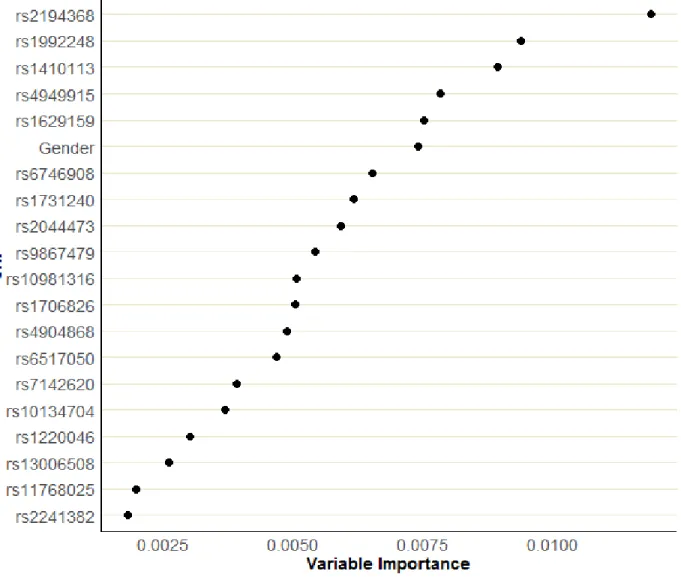
4.1 Variable Importance measures of SNP using the Retrospective Dataset. SNPs are displayed by rank with the most important SNP in the top position. . . 73
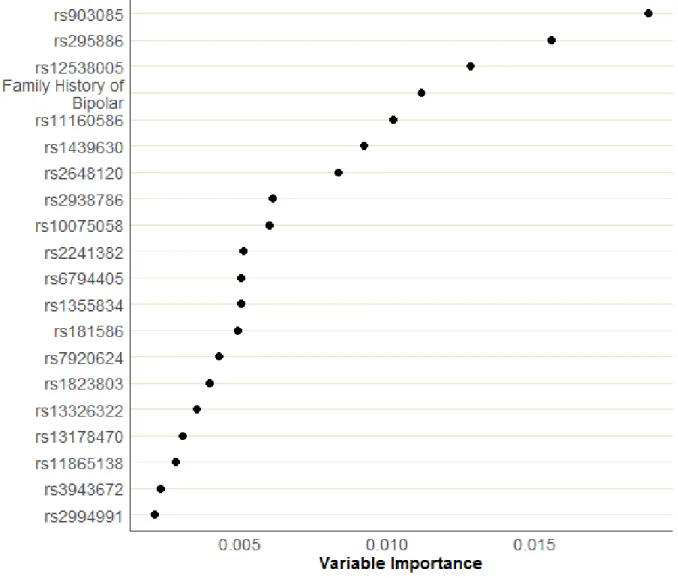
4.2 Variable Importance measures of SNP using the Prospective Dataset. SNPs are displayed by rank with the most important SNP in the top position. . . 74
5.1 Average Variable Importance from Weighted Fuzzy Forests for Diehards . . . . 110
5.2 Variable Importance from Weighted Fuzzy Forests for Tryhards . . . 111
5.3 Weighted logistic odds ratio for Diehards . . . 112
LIST OF TABLES
3.1 Baseline Measurements and Questionnaires . . . 48
3.2 Demographic Table . . . 49
3.3 Comparison of Fuzzy Forests, Random Forests and CART . . . 50
3.4 Results of Module-wise two-step logistic regression and Group LASSO . . . 53
3.5 Comparison of Models using Fuzzy Forests, Random Forests, CART, Module-wise two-step Logistic Regression and group LASSO . . . 55
3.6 Comparison of Models using a 25% hold out sample . . . 56
4.1 Demographic Variables for each cohort by Lithium Response. P values were calculated by Fishers Exact Test . . . 75
4.2 Misclassification rates when subsetting the training datasets by selected demo-graphics . . . 76
4.3 Top 20 Univariate Logistic Regression variables . . . 77
4.4 Full results of univariate logistic regression . . . 77
5.1 Demographic characteristics . . . 102
5.3 Weighted Fuzzy Forests by quitting resolution . . . 106
5.4 Weighted Logistic for Diehards . . . 108
ACKNOWLEDGMENTS
I would like to express my deep gratitude to Professor Christina Ramirez for her support, insight, and endless help in the preparation of this dissertation. I would also like to thank Professor Nandy, Professor Elashoff, and Professor Belin for kindly serving on my doctoral committee and providing suggestions and support during the development of this project.
VITA
2004 B.S. (Mathematics and Statistics), University of Washington, Seattle, WA.
2004-2006 Graduate Student Teaching Assistant, Department of Statistics, Oregon State University, Corvallis, OR.
2006 M.S. (Statistics), Oregon State University, Corvallis, OR.
2006-2008,2013
Special Reader, Department of Biostatistics, UCLA, Los Angeles, CA.
2008 M.S. (Biostatistics), University of California Los Angeles, Los Angeles, CA.
2008–Present Graduate Student Researcher, School of Nursing, UCLA, Los Angeles, CA.
2015–2016 Special Reader, School of Nursing, UCLA, Los Angeles, CA.
PUBLICATIONS
A Nyamathi, B Salem, E Hall, T Oleskowicz, M Ekstrand, K Yadav, J Toyama, S Turner, Susan M Faucette(2017). Violent crime in the lives of homeless female ex-offenders. Issues in mental health nursing, 38(2), 122-131.
A Esguerra-Gonzales, M Ilagan-Honorio, S Fraschilla, P Kehoe, AJ Lee, T Marcarian, K Mayol-Ngo, PS Miller, J Onga, B Rodman, D Ross, S Sommer, S Takayanagi, J Toyama, F Villamor, SS Weigt, A Gawlinski(2013). CNE article: pain after lung transplant: high-frequency chest wall oscillation vs chest physiotherapy. Am J Crit Care22(2):115-124.
A Esguerra-Gonzales, M Ilagan-Honorio, P Kehoe, S Fraschilla, AJ Lee, A Madsen, T Mar-carian, K Mayol-Ngo, PS Miller, J Onga, B Rodman, D Ross, Z Shameem, K Nandy , J Toyama, S Sommer, C Tamonang, F Villamor, SS Weigt, A Gawlinski(2014). Effect of high-frequency chest wall oscillation versus chest physiotherapy on lung function after lung transplant. Appl Nurs Res.27(1):59-66.
K De Azambuja, P Barman, J Toyama, D Elashoff, GW Lawson, LK Williams, K Chua, D Lee, JJ Kehoe, A Brodkorb, R Schweibert, S Kitchen, A Bhimani, DJ Wiley(2014). Validation of an HPV16-mediated carcinogenesis mouse model. In Vivo28(5):761-767.
NA Pike, CA Okuhara,J Toyama, BP Gross, WJ Wells, VA Starnes(2015). Reduced pleural drainage, length of stay, and readmissions using a modified Fontan management protocol. J Thorac Cardiovasc Surg150(3):481487.
SV Godbole, K Nandy, M Gauniyal, P Nalawade, S Sane, S Koyande,J Toyama, A Hedge, P Virgo, K Bhatia, RS Paranjape, AR Risbud, SM Mbulaiteye, RT Mitsuyasu(2016). HIV and cancer registry linkage identifies a substantial burden of cancers in persons with HIV in India. Medicine95(37).
CHAPTER 1
Introduction
Nursing bridges the gap between doctors and patients, not only in terms of care but also of information. Nurses not only help during surgeries and implementing new hospital wide policy changes but are critical to elevating the quality of life of patients. With such a diversity of settings and opportunities to create changes in the medical field, nurses have the potential to create and guide their corresponding specialized fields forward. The wealth of data generated through electronic medical records and through patient responses on ques-tionnaires offer great promise of individualize health care and improved] patient outcomes. This deluge of information often is of high dimension and also is often correlated. This can pose problems with traditional methods. Much of the time, the data cannot be utilized completely as is, but instead requires previous research to guide researchers to choose rele-vant predictors prior to model selection. Traditional methods such as logistic regression and mixed models cannot necessarily converge and struggle with identifiability when the number of measurements collected approach or become larger than the number of patients in the study. Unfortunately this commonly occurs among nursing data. The following explores two situations where a number of measurements were taken and that traditional methods were used, but where alternative methods may have been able to offer additional guidance.
Machine-learning techniques along with traditional techniques can help shed light in these situations. We concentrate on decision trees in particular because of their relative ease of use, availability and predictive ability. Random Forests also have favorable predictive pro-files when compared to other methods such as support vector machines and neural networks
([70], [49]). With the usage of R and SAS that have packages or add on packages available to the user, random forest is widely used, parallelizable and computationally efficient.
The next sections will present selected decision-tree based machine-learning methods, CART, Random Forest, Conditional inference trees, and Fuzzy Forests. Main concepts from each method will be presented from each of these ensemble methods.
1.1
CART
The base learner of our decision tree forest is Classification and Regression Trees (CART). The applications and extensions presented in subsequent chapters will be limited to the situation where the outcome is categorical, although it extends easily to the regression setting with continuous outcomes. When the outcome is categorical and made up of a set of classes, a classification tree can be used to produce a tree or model to predict what outcome class results from each of the branches or partitions in the data. In classification tree based methods, the purpose of a tree is to provide a sequence of decision rules that can be used to partition the observations such that each partition makes observations within the contained area as similar as possible.
1.1.1 Characteristics of a Tree
Each tree is comprised of nodes and branches where each node consists of a subset of the observations and a branch further partitions the data. The starting node, also known as a root node, contains all the observations in the sample and the internal nodes are repeatedly partitioned until a tree is fully grown and a terminal node is reached. The terminal node represents a point where some stopping criteria has been employed, the node only contains one observation, or all the observations in that node all have the same outcome.
Starting at the root node, each node is split into two groups, called daughter nodes, according to some decision rule that consists of a variable and a split point. Both the right and left daughter nodes are split such that each subset of the data at each node contains a high frequency of the same outcome class, ideally with all the observations in a node of the same outcome class (pure node). Each split is interpreted as a condition set on the selected variable, for example if the decision rule for a particular node is Age ≤ 5, then any individual that is age 5 or younger is partitioned into one daughter node and everyone older than 5 is in the other daughter node. Each daughter node then goes through the same process of choosing a variable and split that partitions the data into smaller and smaller subsets. Continuing the example described earlier, if the node made up of those older than 5 is followed by a branch that splits the node by gender, then that branch describes a partition that includes females older than five and another partition of males older than five. The recursive framework keeps going until a terminal node is reached. Since each partition is easily interpreted and the overall tree itself is a combination of decision rules describing a specific set of characteristics, these set of rules that can be a very valuable tool in the decision-making process. The hierarchical nature of a tree naturally include interactions that do not need to be known a prior, allowing for very flexible models.
1.1.2 Growing a Tree
The selection of the variable and split utilizes a multi-step selection method that chooses the best possible variable and split among all the predictors in the data. CART is able to identify among the continuous and categorical predictors, for each node, the optimal variable and split point which results in the largest decrease in impurity. The number of possible splits being considered vary by the type of predictor being considered. The possible number of splits for every categorical variable with q categories is 2(q−1)−1 [42]. If the variable is continuous with k different observed values, there are k-1 midpoints between the observations to be considered before the decision rule can be determined [13]. To determine
which of these possible splits to select, the splitting rules are ranked and the rule that maximizes the decrease in node impurity is selected.
The purity of each node depends on the proportion of each class in the node. The node is pure when a node is entirely composed of one particular class and most impure when the proportion of each class is equal. The resulting splitting rule maximizes the difference between the node impurity in the parent node and the sum of the impurity in both the right and left daughter nodes [42]. There are multiple measures of the node impurity used to make this determination with a few common methods utilizing either the GINI index or other deviance measurements such as entropy. Once the node is split according to the chosen variable and split-point, each of the resulting daughter nodes are partitioned such that the next best variable and split is chosen from among the remaining predictors not already used in that branch. For example if there are X1, X2, X3, X4 predictors and some cutpoint inX1 is chosen at the first split and some cutpoint inX2 splits the subsequent right daughter node then the choice ofX2 is based off the resulting partition created by the split in X1 and any other predictor that would have come before it in that branch. The following equations and related notations are adopted from the text in Hastie et. al. [42]. In growing a classification tree, let Rm represent a node m with Nm observations. Let k(m) represent the majority
class in node m andPm represent the proportion of class k observations in node m, with the
estimated Pm taking the following formula:
ˆ
Pmk = (1/Nm)
X
xiRm
I(yi =k). (1.1)
The GINI index and deviance measure impurity in the node by utilizing the proportions of each of the classes in the following formulas, respectively
X k6=k0 ˆ PmkPˆmk0 = K X k=1 ˆ Pmk(1−Pˆmk). (1.2) − K X k=1 ˆ PmklogPˆmk. (1.3)
Misclassification rates can also be calculated for each tree to measure overall predictive accuracy of the tree and utilizes the majority voting scheme to determine how often an
observation was incorrectly classified to a particular class[42]. The majority voting takes the class representing the highest percentage in the node and assigns it to every observation in that node using the formula
(1/Nm)
X
iRm
I(yi 6=k(m)) = 1−Pˆk(m),m. (1.4)
1.1.3 Pruning a Tree
If the resulting tree is very large, the model complexity may over fit the data and if it is too small it may not grasp the important interactions present. Pruning can prevent a model from overfitting the data by removing selected lower branches in the tree. Hastie et. al [42] describe the following cost complexity function, which if minimized, balances the size of the tree with the goodness of fit to the data. This is better than a hard and fast alternative rule for always removing branches that do not achieve some threshold, which can potentially result in interesting relationships being ignored. Since GINI is more sensitive to changes in node probabilities, it is commonly used while growing the tree, whereas the misclassification rates are commonly used for the cost complexity pruning of the tree where the cost function is defined as follows:
Cα(T) =
|T|
X
m=1
NmQm(T) +α|T| (1.5)
with T indicating any sub tree, |T| denoting the number of terminal nodes in T, α repre-senting the tuning parameter that balances the tree size and its goodness of fit to the data, and Qm signifying the measures of node impurity. Hastie et. al. describe how to minimize
this cost function to produce the optimal tree from the maximal or largest possible tree grown from the data. To minimize the cost function, one must first estimate the tuning parameter α using a 5 or 10 fold cross validation. To do this, either subset the data into 5 or 10 partitions, omitting out one subset at each run on which to test your model. For each run, use the remaining data as a training set to grow the tree and calculate the |T|
test the various values obtained from the test data to determine which α value provides the smallest prediction error. Using these α values, determine the subtree that minimizes the cost function. Subsequently prune the trees so that the values of |T| are reflected and determine which results in the smallest prediction error [42]. In the case where there are missing values and no split point is able to be determined, a surrogate variable may be used. Surrogate variables are predictors and split points that are utilized when there are missing observations in the primary-splitter variable. A surrogate is chosen if they are close to the primary splitter, where the closer they are together, the smaller the information is lost at that split [42].
1.1.4 Variable Importance
Variable importance measurements for the list of parameters are calculated as the decrease in impurity attributed to that variable. The importance of a variable is the sum of the decrease in impurity across all the nodes where that variable was chosen as the primary splitter or as a surrogate splitter[71].
After the tree is grown, the observations in node q are assigned to a class k(q). As a data mining technique, CART is easily utilized for large datasets to classify data into their respective groups. While CART can also handle missing data for its non-parametric and nonlinear categorizations, there are still limitations to this approach [42]. One such limitation is that CART tends to be susceptible to over-parameterization and the resulting prediction can be unstable. This instability is due to the fact that a single tree has high variance, which means that a change in the data may affect which variable is chosen at the first split and then that change is pushed further down the tree [42].
1.2
Random Forests
A single CART tree is known to be unstable, that is small changes in the input data set can lead to difference in prediction. Combining individual models can create ensemble predictors that improve the accuracy and stability of the model. Ensemble predictors, are a supervised learning technique that combines weak classifiers, which can be models that are only slightly better than random guessing, such that the new combined strong classifier has a higher accuracy than each of the individual weaker classifiers[63] .Ensemble predictors display the most improvement when there is high variability between individual models that can be used to smooth out the decisions produced by any single model ([32]).
1.2.1 Bagging
Bootstrap aggregating, also known as bagging, was developed to reduce variance and prevent model over-fitting. Bagging applies a learner to bootstrapped samples of the data, which have been bootstrapped with replacement. If applied to the decision trees, bagging averages the outputs from the repeated bootstrap samples of the data [21]. Averaging produces much more stable estimates, particularly since a bootstrap sample taken with replacement is expected to only have 63.2% of the original data. Through aggregation, Bagging is able to reduce the variance by averaging the prediction over multiple bootstrap samples. In the classification tree setting, B bootstrap samples are selected from the data with B subsequent tree classifiers produced from each tree. The misclassification rate is taken to be the proportion of times the predicted class is different from the true class and averaged across all the classifiers. While bagging works well in increasing precision of highly unstable classifiers, it may potentially result in a worse classifier when the original classifier is already relatively stable[22].
1.3
Random Forest
Random forest is an ensemble classifier developed by Leo Breiman(2001) and is built upon the premise that you can get better performance by de-correlating the trees obtained by Bagging. In Random Forests,B Bootstrap samples are constructed with replacement. To add further randomness and to aid in de-correlating the trees, at each node in building the tree, the best split is chosen from a subset of all possible parameters of size mtry selected at that node. If mtry =pthen, random forest reduces to bagging. Increasing the randomness results in a set of trees that have low correlation and can produce good predictive accuracy and more stable results[23].
It is important to note that each tree contributing to this ensemble classifier is grown without pruning so as to create more variability in the forest. Mtry is an important tuning parameter and locating the optimal mtry is necessary in finding the best model ([23]). This is especially true in high dimensional problems. The size ofmtry must be large enough such that important predictors have a high probability of being chosen within the set.
1.3.1 Random Forest Algorithm
For b = 1 to B:
1. Draw a bootstrap sample of size N from the training data.
2. Grow a random forest tree Tb to the bootstrapped data, by recursively repeating the
following steps until the minimum node sizenmin is reached indicating a terminal node
of the tree.
• Selectmtry variables at random from the p variables.
• Split the node into two daughter nodes 3. Output the ensemble trees TbB1
1.3.2 Out-of-Bag Estimates
Breiman’s Random Forest paper includes explanations on how the prediction error is calculated. Bagging is used in the construction of each tree and corresponding classifier. Given a training set T, the classifiers are constructed from the B bootstrap training sets obtained from T and the resulting bagged predictor is calculated from the majority votes. For each X,Y in T, the combined votes over those classifiers which do not contain X,Y are calculated and are called the out-of-bag(OOB) classifier. The generalization error can then be estimated by calculating the error rate for the out-of-bag classifier. In calculating as such, this prevents the need for a testing data set. Since the bootstrap sample excludes approximately third of the data, the resulting OOB estimate only includes about one-third of the data points, which can lead to overestimating the current error rate. The OOB error estimate takes the proportion of times that the class with the majority votes is not the true class, averaged over all cases. However, unlike in cross validation, the OOB estimate are unbiased if the estimate is calculated well after the test set error converges[23].
1.3.3 Variable Importance
Variable Importance is estimated through the tree-building procedure. There are two common methods for determining variable importance in random
forests: GINI and permutation importance. The first, which is the default for most statistical packages, is for the split at each node to be determined based on the GINI impurity criteria, where 0 or 1 represent a pure node and 50-50 (in the case of a binary variable) represents the most impure node. The GINI variable importance for variable Xi sums across all trees
the decrease in GINI between the parent and the two daughter nodes for those splits made on Xi [6]. However, utilizing this measure does show a preference for predictors with many
possible splits or categories.
This second method is permutation importance, and will be the one that will be focused on in this manuscript. This method uses a permutation framework to calculate the variable importance measurements and changes in prediction accuracy. Calculation of the permutation importance, starts with randomly permuting the OOB cases of Xi in
each tree. The other predictors along with this permuted variable are then used for the OOB observations to predict the response. Then the difference in the number of votes for the correct class in the original sample and the permuted sample is computed with the rational being that accuracy will be diminished when an important variable’s connection with the outcome is obfuscated. The formula and all related variable definitions for the permutation importance is presented from Strobl et. al’s paper on Conditional variable importance for random forests[74] which is illustrated by (equation 1.6). The permutation variable importance measure for Xi is the average permuted difference across all the trees.
The idea is that permuting the Xi variable will break the correlation to the response and
produce a more accurate measure of variable importance. The permutation importance is more commonly used due to the biased variable preferences that the GINI index tends to produce. Also, when building the forest, the size of the forest can affect the stability of the permutation importance and the larger values ofmtry can result in a large permutation importance [87]. Formally, let
V I(t)(Xj) = P iβ¯(t)I(γi =γi(t)) |β¯(t)| − P iβ¯(t)I(γi =γi,πj (t)) |β¯(t)|. (1.6)
Equation 1.6 takes ¯β(t) to be the OOB sample for tree t and γ
i(t) = f(t)(Xi) is
the predicted class for observation i and γi,πj
(t) = f(t)(X
i,πj) is the predicted class after permutation. Using this formula the permutation variable importance measure is calculated as
V I(Xj) = Pntree t=1 V I (t)(x j) ntree (1.7)
This calculation for variable importance looks at the magnitude of the difference between the original prediction error and the prediction error once the values for that variable are permuted [75]. The stronger a signal or the more informative that variable is, the higher in the tree that variable will appear. Since the subsequent branches are conditional on the variables selected higher in the tree, any changes to important variables at the top of the tree can result in a larger effect on the overall prediction accuracy of the tree.
The variable importance averaged across the trees can also be standardized to be used in hypothesis testing. This overall variable importance measure for each variable can be transformed into a scaled variable importance measure by dividing the variable importance by the standard error ˆσ/p(ntree) [75]. This scaled variable importance measure now has a standard normal distribution which can be used in hypothesis testing to determine if the variable importance score is significant at an alpha level.
1.3.4 Proximities and Applications
A useful measure that is calculated from the random forest algorithm is the proximity matrix. The proximity matrix indicates how close two observations are to each other. The (i,j) element in the proximity matrix is the average number of trees that have observations i and j end up in the same terminal node [48].
Random forest also has methods to deal with potentially large amounts of missing data. In Breiman’s seminal paper([23]), he proposed a rough fix to deal with missing values in the data. The proposed method is simplistic and substitutes the median value for the continuous variables and takes the class with the majority votes for the imputed categorical value. Comparatively, a more adaptive method could utilize the proximity matrix that
is already calculated from random forest. To take advantage of this calculation, random forest package in R [61] is grown using the data with the missing values filled in using the simplistic method. In the package, the rough imputed values are then updated using the proximity matrix as weights. For continuous variables, the R function updates the imputed values using the matrix as the weights and taking the weighted average of the non-missing observations. Similarly, the package takes the categorical variables take the maximum value from the proximity matrix that corresponds to that variable.
Along with handling missing data, the proximity matrix is useful in determining outliers. For a specified class, low proximities relative to the others in that class, may be indicative of an outlier [6].
1.3.5 GINI bias
Even though CART and other decision tree methods commonly use the GINI index to determine the best variable and cut-point to use in growing the tree, Strobl’s 2007 paper [73] indicates that the GINI measurement can be biased. In fact, Strobl indicates that the estimate of GINI does not produce an unbiased estimator and results in preferences for correlated and/or continuous predictors. If N represents the sample size and p corresponding to the proportion of the majority class in that node, the estimate of impurity, namely the GINI index, underestimates the true GINI index by a factor of (N −1)/N. Also, the paper indicates that the expected change in GINI( ˆ∆G) between the parent and daughter nodes is equal to 2p(1−p)/N. Therefore, under the null hypothesis that the change in GINI is 0, ˆ∆G has a positive bias that is a function of the sample size. When the predictors have different sample sizes, there is a bias towards those with many missing values (smaller number of non-missing observations). Strobl’s paper also indicates that by testing multiple cutpoints to find the optimal split, a multiple testing situation occurs that serves to increase the type I error rate. For the splitting selection situation, the type I error is when a variable is chosen for splitting even if it is just a noise variable. In the decision tree situation with binary
splits, the number of comparisons that need to be performed to determine the optimal split depends on the number of possible splits of that variable. This means that as a result of all the multiple comparisons, variables with many categories or continuous variables twill be chosen more frequently when the GINI index is used to measure impurity [73]. The next section will deal with this issue.
1.4
Conditional Inference Forests (CIF)
It is known that Random Forest variable importance is biased towards correlated predictors [75]. Highly correlated variables arise in many situations, especially in biologic and genomic studies where variables can be subsets or even linear combinations of vari-ables. Biologic and genomic studies often have many more predictors than observations, thus machine-learning techniques such as Random Forests are often used for feature selection. In Strobl’s paper [75], a conditional variable importance measure was proposed to address this limitation and reduce biased variable importance measures produced by the Random Forest algorithm. Their main focus was on distinguishing between the marginal associations that produce relatively high variable importance and the more informative associations present once conditioning on other predictors. Strobl’s method builds upon the work done to produce CARTscans plots that output marginal influence along with conditional influence plots for categorical predictors. The rationale for conditional variable importance measures stem from the fact that both the permutation importance and the GINI importance measures indicate marginal associations and thus may be misleading. By conditioning on other predictors in the data, insights into the real relationship between the variable of interest and the outcome will be availed. By conditioning on other predictors in the data, the variable importance measure can break free from the preference of correlated predictors to be chosen in early splits, which translates into a higher variable importance score. The situation using decision trees lends itself nicely towards a conditional framework. Since at any node, the prior splits in a branch describe a pattern of predictors and splitting criteria, that node can be thought
of as conditional on only those particular variables seen prior to it in its branch. The only exception is at the first split, when there is no other predictors prior to it to condition on [75].
1.4.1 Conditional Inference Trees
The basis upon which conditional permutation Random Forests is built hinges on the unbiased tree method proposed by Hothorn, Hornik and Zeileis in 2006 [44]. Their method proposes a two-step procedure that separates the variable selection from the cutpoint selec-tion used to partiselec-tion a node into it’s two daughter nodes. Hothorn’s paper illustrates that separation of the variable selection and the cutpoint determination does well in preventing the tree algorithm from preferentially choosing categorical variables with many categories or variables with many missing values. Their paper describes how using hypothesis tests to determine the stopping criteria allows the predictive accuracy to be the same as that from an optimally pruned tree while preventing overfitting. However this aspect of the separation in determining the decision rule is not as important in this situation since averaging the trees takes care of any overfitting that any one individual tree may have[44].
The following description of the steps utilized to determine what variable and split point to use at each node is presented from Hothorn’s paper [44]. A two-step method is described with the variable selection step testing the global hypothesis of independence between any of the covariates and Y. The hypothesis is made up of p partial hypotheses that test the hypothesis that the distribution of Y given the covariate is the same as the marginal distribution of Y, with the global hypothesis looking at all of the covariates. The association is measured by permuting the responses and a function of the covariate being tested. The p-value from each test is obtained using the permutation framework that fixes the covariates and conditioning on all the possible permutations of the outcome. If the global hypothesis fails to be rejected at some αlevel, then the node is not split and becomes a terminal node. If it can be rejected, then the covariate with the strongest association with
the outcome is chosen to split the node. Once the variable is chosen, the next step determines at what cutpoint to split the variable. Once the best predictor is selected, then the cutpoint selection is selected by again doing a permutation test. The potential cutpoint splits the observations in the node to form two subsets of the observations for that node. The split that corresponds to the case where the permutation test maximizes the difference between the prediction permuted for each subset of the node, is the one chosen for the splitting criteria [44].
1.4.2 Cforests
Strobl et. al.’s 2008 paper on conditional variable importance for random forests[75] goes into detail regarding the rationale behind the conditional framework for the permutation variable importance. Since permutation variable importance may lead to spurious associa-tions, consider it in terms of permutation tests. With a global test, the null hypothesis is that Y is independent from all the other predictor variables in the data. This translates into the null hypothesis that the permutation of Y has no effect on f(y) or on f(X1, X2, ...Xp).
This implies that when the permutation importance shows a significant difference in the joint distribution of Y and X1, ...Xp, that either Xj is not independent of Y or that the Xj
is not independent of the other p-1 covariates. In determining how influential Xj is on Y,
the relationship betweenXj and the other p-1 covariates are not of interest. To achieve this,
a conditional permutation scheme only looks at if Xj and Y are independent instead of if
Xj is independent of both Y and the p-1 covariates. This is done by permuting Xj only
among the observations that have the same values in each of the p-1 covariates to maintain the same correlation structure among the predictors. The null hypothesis now is that Xj is
independent of Y given X1, ...Xj−1, Xj+1, ...Xp. If we let Z = X1, ...Xj−1, Xj+1, ...Xp then
Ho: (Xj ⊥Y)|Z. Under this null hypothesis the following conditional results.
If Xj is correlated with Z, then the differences in the distributions are a result of
such correlation and not the relationship of interest and thus leads to the preference in the variable selection and overestimates the permutation importance. Also by permuting within groups of observations with Z = z, this maintains the correlation structure of Xj and the
other covariates. The resulting unbiased conditional permutation trees are used to define the partitions upon which the permutations will be done. This provides a readily available partition grid that has already been determined by the algorithm[75].
1.4.3 Cforest Algorithm
The following algorithm is presented from Strobl’s paper [75].
1. For each conditional permutation tree, compute the OOB prediction accuracy before the permutation of Xi. P iβ¯(t)I(γi = ˆγ (t) i ) |β¯(t)| (1.9)
2. For each of the variables Z to be conditioned on, obtain the cut points that split the variable in the current tree. Then obtain the partition by using each of the cut points sequentially.
3. Within the partition grid, permute the values ofXi and determine the OOB prediction
accuracy using the following formula: P iβ¯(t)I(γi = ˆγ (t) i,πj|Z) |β¯(t)| , (1.10) where ˆγi,π(t) j|Z =f (t)(X
i,πj|Z) is the class that was predicted after permutingXj over the partition structure.
4. The average difference between the prediction accuracy of the unpermuted and the permuted grid, computed across all the trees, results in the permutation variable im-portance.
1.4.4 Partition Grid
To determine what variables to condition on, Strobl’s paper recognizes that a natural choice would be to take advantage of the model already created from each of the individual conditional inference trees grown in the forest. The paper proposes that each of the trees can be thought of as a series of binary splits that produces at least one cutpoint for each variable that can be used of as a partition grid. However since each of these cutpoints are based on nodes within a branch, Strobl notes that bisecting that variable does not necessarily split the sample space but can result in partial planes and can make things too computationally intensive. Instead of using a cutpoint specified at each node, Strobl suggests using the cutpoint, regardless of whether it is based on a continuous or categorical predictor, as a bisector of the sample space to produce a simpler grid. Also as a way to alleviate some of the computational burden, Strobl proposes only using those predictors correlated above a certain threshold with the variable of interest to be conditioned on. The partitioning method could result in a grid that contains some small cell frequencies. Strobl indicates that while this is was not a problem in her simulation studies, the small cell frequencies only add to inducing greater variation for the resulting ensemble predictor[75].
One caveat to this method is that mtry has a strong influence over the effectiveness of this variable importance measure. Selecting an mtry of 1 results in a random variable selection regardless of whether the permutation or conditional importance measures were used [75]. On the other hand, a high mtry will allow a conditional permutation to have the most effect at preventing spurious relationships, it will also result high variability in the values of the importance measurement Strobl [72]. But regardless of whatmtry is chosen, the conditional permutation framework results in a similar pattern but with a lower variability than the permutation importance, which in turn may help with identifiabilityStrobl [72]. The biggest caveat with this method is its computational intensiveness. It is not feasible for even moderate sized datasets.
1.4.5 Variable Importance Bias
Strobl’s 2008 paper also acknowledges that while the conditional permutation results in less biased importance scores as opposed to using the GINI index, the conditional variable importance algorithm still resulted in the uncorrelated predictor variables being selected less often and with a lower importance in the hierarchy of the tree and thus resulting in a low variable importance measure. The tuning parameter mtry, as mentioned before, is also highly influential, with a low value preferentially choosing correlated predictors and a large value increasing the variability of the importance measure.
Another study done by Nicodemus and Malley(2009) also aimed to deal with the issue of variable importance bias. Their study found that Random Forest preferentially selected correlated predictors when the selection was obtained using the GINI index and conditional inference forests tended to overweight the uncorrelated variables. They also found that conditional inference forests were computationally infeasible for moderate to large datasets [53].
1.5
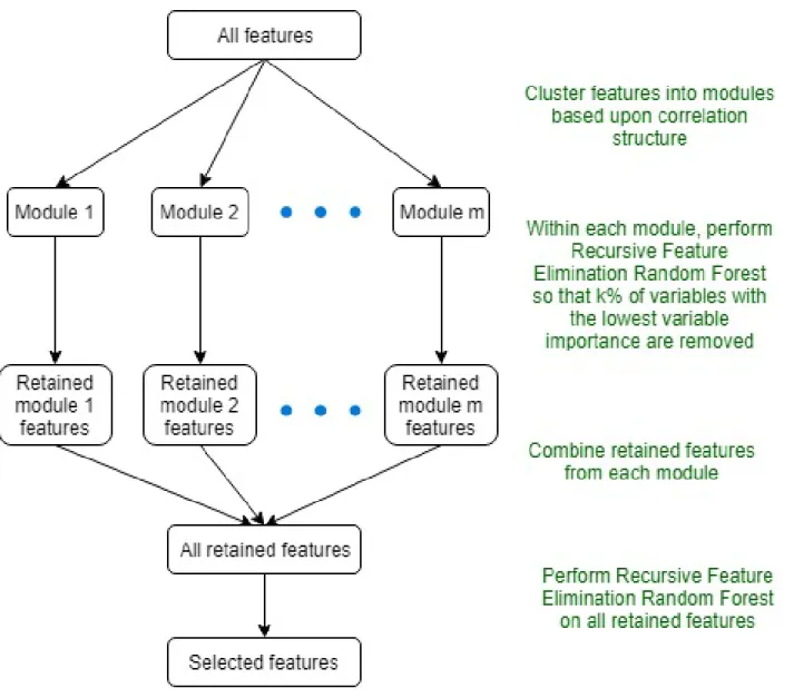
Fuzzy Forest
Fuzzy Forests and all related concepts described below are presented by Conn et. al.’s paper Fuzzy Forests: Extending Random Forests Algorithm for Correlated, High-Dimensional Data [28]. Fuzzy Forests is a screening algorithm to find the most important variables when there exists correlated variables along with independent variables, especially when the number of parameters greatly exceeds the number of observations. Fuzzy Forests is a two-step process that utilized both unsupervised and supervised learning. The process starts with unsupervised learning where a weighted correlation network separates the feature space into modules, such that only the features within a module are highly correlated and there is low correlation between modules [28].
1.5.1 Module Selection
The first step is constructing a weighted correlation network construction or module creation. The discussion requires that some key network concepts be addressed. The first concept that needs to be explained is ”‘approximately scale-free”’ networks. Barabasi and Bonabeau[17] explain that some networks, such as those modeling relationships between sex-ual partners, portray a network that contains some individsex-uals with few partners and others that are hubs with hundreds of partners, are called ”‘scale-free”’. ”‘Scale-free”’ is used to loosely describe some hubs’ ability to have seemingly endless links and no node is typical of the others. In the past, complex networks were thought to be completely random and are characterized by all nodes having approximately the same number of links. In this setting, the distribution of the number of connections for each node follows a Poisson distribution. However, in many real life networks, the ”‘scale-free”’ setting, is more appropriate. These networks indicate that the probability that a node has k links follows a power law distribu-tion and is propordistribu-tional to 1/k. Unlike the Poisson distribudistribu-tion used to describe random networks, which does not allow for hubs, the power law for the ”‘scale-free”’ networks al-lows for networks in which a few hubs dominate. In many real life situations, the random networks ignore hubs and fail to describe what is truly occurring due to the underlying as-sumption that all nodes are equal and existed before the links were made. However, in real life networks that are constantly evolving, older nodes have greater chances to gain more links and preferences are placed on certain nodes(ex. people are only familiar with a small portion of the internet and choose from a tiny subset of the more popular sites because they are easier to locate) [17]. Another simple example are airline networks where most flights originate from several hubs such as LAX, JFK, DFW etc.
Formally, Barabasi describes scale-free networks [60] as any network where the prob-ability of a node having k links to others in the network follows a power law distribution which is Ck−γ, with C being a constant and γ is the degree exponent. Barabasi indicates
smallest k for which the power law holds. When k is continuous, the normalizing constant C is represented by (γ −1)kminγ−1. When k is continuous, p(k) does not indicate the proba-bility that a randomly chosen node has degree k like it does when k is discrete, instead the probability can only be defined within a range ofk1 to k2. In this case, the probability that a node has a γ between k1 and k2 is defined as
Rk2 k1 p(k)dk = (γ−1)k γ−1 min Rk2 k1 k −γdk.
Barabasi also indicates that the natural cutoff or the size of the largest hub is calcu-lated as
kmax=kminn
1
γ−1 (1.11)
where n is the total number of nodes, and indicates that the larger the network, the larger the hubs become. In most real networks,γ is≥2 since γ−11 >1 in thekmax formula whenγ <2.
If this were the case, this would mean that the number of connections to the largest hub would grow faster than the size of the network. γ is usually between 2 and 3. γ in this interval only have finite first degree moments and all higher order moments diverge as limn→∞. When γ
exceeds 3, these networks resemble random networks. As a result, ifγ >3 then the required network size needed for a scale-free network is a transformation of (1.11) to n = (kmax
kminγ−1. For
example if γ = 5, kmin ≈ 1, and kmax ≈ 100 then a scale-free network would require at
minimum 108 nodes, which most networks are not [60]. Zhang and Horvath [86] proposed an easier method usingR2, which is the square of the correlation between log(p(k)) and log(k), to determine if a network approximately has scale-free topology. These network characteristics along with other network concepts will help to determine the groups of variables or modules in the network. Zhang and Horvath use their criteria for approximate scale-free topology along with other network concepts to present an overview of module selection. Zhang and Horvath describes the network topology as a graphical representation of a network, where the vertices are the variable and the edges are the interactions between them. Two variables are connected in a co-expression network if the co-expression, measured using some measure of similarity such as Pearson’s correlation coefficient, is above some threshold. The co-expression network links to an adjacency matrix, which indicates the connection strength between variables. The correlations between corresponding variables are calculated as a
similarity matrix, which is then altered into the adjacency matrix. The adjacency matrix is then used to represent node dissimilarity, which will serve as the input data upon which the variables will be clustered into modules or clusters of variables [86].
Zhang and Horvath describe an adjacency function which uses Pearson’s correlations from the similarity matrix to create the adjacency matrix. The adjacency function can utilize either a strict cut-off, which is known as a hard threshold, or the more flexible, soft threshold. The most common adjacency function for hard thresholding is
aij = 1 ifsij =cor(i, j)≥τ 0 ifsij =cor(i, j)< τ
with τ being the hard threshold. Some suggestions for the estimation of τ utilize the sig-nificance level of a correlation, which in turn thresholds the p-value corresponding to the correlation coefficient. The size of the network decreases as a function of the threshold [86]. An alternative method uses the relationship between the network size and the correlation threshold and sets the network size as a constant [19]. Hard thresholding has an intuitive interpretation since it represents the number of variables that are directly connected with an edge(first order interaction), but the lack of flexibility does not recognize those connections that are close to the threshold cutoff [86].
Zhang and Horvath’s paper describes a soft thresholding function such as the power adjacency function, is given as aij =| sij |β, where β is the soft threshold . The power
adjacency function can be used to express a weighted correlation network. It also has a fac-torization property that preserves the facfac-torization of the correlations such that ifsij =sisj
thenaij =aiaj with ai = (si)β. Estimating the β parameter in the soft-threshold is different
from that for the hard-thresholding. In this case, the soft-thresholding parameter uses the scale-free topology criteria, which only considers networks withR2 > .8. Since β values that result in a R2 value close to 1 may show networks with very few connections. Additional considerations should include a high mean connectivity to ensure enough information for module creation, and that the slope of regression line between log(p(k)) and log(k) should
be close to -1.
Following the adjacency matrix calculation Zhang and Horvath describe how the topological overlap measure is computed. They measure the overlap in the variables with strong connections to both variables i and j. These values populate the topological overlap matrix (TOM) and is calculated as
wij = lij+aij min(ki,kj)+1−aij if i6=j 1 else
In this formula, lij =Puaiuauj and node connectivity is represented by ki =Puaiu,
which represents the variable connectivity by taking the sum of the ith row in the adjacency matrix. Under the hard thresholding,lij represents the number of variables that the ith and
jth variables are both highly correlated with. The topological overlapwij is 0 when there is
no variables common to both the ith and jth variables. Similarly, wij is 1 when all of the
neighbors of the ith node is the same as those of the jth node. As a result of how the wij
is calculated, the TOM is non-negative and symmetric. The TOM is then transformed into a dissimilarity matrix by taking each element in the matrix and subtracting it from 1. The TOM dissimilarity matrix is then used to determine the modules [86].
Once the TOM dissimilarity are computed, the modules with high topological overlap can be determined [86]. The modules are determined using average linkage hierarchical clustering. The following description by Sayad, describes hierarchical clustering creating clusters based on prior clusters ([2]). Hierarchical clustering groups all the variables divisively by starting with one cluster and then recursively partitions the cluster into two groups that are the most dissimilar, until there are n clusters. The agglomerative method is another hierarchical clustering method where each node is its own cluster. Then a similarity measure is computed between each cluster and similar clusters are combined. Successive clusters are combined until a single cluster is formed. Horvath’s book on weighted network analysis
describes clusters being combined using the pairwise dissimilarity measure [43]. The linkage method or inter-cluster dissimilarity is calculated between each pairwise nodes in the clusters. Horvath’s equation on average linkage hierarchical clustering is computed as
daverage(clust.q1, clust.q2) =
P
i∈clust.q1 P
j∈clust.q2di,j
|clust.q1||clust.q2| (1.12)
di,j represents the pairwise dissimilarity between the ith and jth node and | clust.q1 | and
| clust.q2 | is the number of objects in the two clusters. For illustrative purposes, Horvath indicates that the results of agglomerative hierarchical clustering as being represented in a dendrogram, with nodes (x-axis) combined at each step and the height(y-axis) of each step indicates the dissimilarity of the merged nodes. The number of merges is less than n−1, with the heights at each merge increasing. The resulting plot resembles a tree where the branches correspond to clusters and nodes as leaves. The nodes and corresponding branches are organized such that the lines in the dendrogram do not cross [43].
Once the dendrogram is created, Zhang and Horvath [86] describes the module cre-ation where branches in the dendrogram depict the different modules. The TOM plot uses the TOM-based dissimilarity values to create a dendrogram. A Topological Overlap Matrix Plot sorts the nodes by the hierarchical clustering tree and represents the TOM dissimilarity values utilizing complementary colors. Since the TOM-based dissimilarity matrix is sym-metric, as is the TOM plot, the modules are represented by high overlap, which is found along the diagonal [86].
1.5.2 Recursive Feature Elimination with Random Forests
It is important to note that the weighted correlation network in the first step is done without the outcome variable, that is, it is unsupervised learning. Once the modules are formed, variable screening using recursive feature elimination on each module is used to reduce the parameter space of each module.
Diaz-Uriarte and Alvarez de Andres [31] proposed an iterative Random Forest method. Their method entails iteratively building Random Forests and removing those variables with the smallest variable importance, such that the resulting subset of variables produces the smallest OOB error rate. For this procedure, the OOB error is used solely to select the final set of variables and not for estimation purposes, since the usage of the OOB in the iterative approach results in the OOB being biased down. This is similar to the rationale for the ”‘selection bias”’ explained by Ambroise and McLachlan [14]. In it, they describe that a cross validation or the bootstrap method[33] should be utilized to correct for the selection bias resulting from the feature-selection process.
The selection bias described by Ambroise and McLachlan [14] arises from which vari-ables are used to perform feature selection in the training of the classifier. When the data is partitioned into a training and test set, a selection bias results due to the fact that the test error is based on the test set, which is a subset of all the variables used to create the classifier. The end result is that the test error is larger than the prediction error. For example, if three genes are selected, they report that the data is split into a 95/5% for the training and test sets, respectively. Fisher’s linear discriminant rule had an average test error or 10.7 and 0% [14].
Fisher’s linear discriminant function classifies the data into two groups, where each group are classified based on k variables. The data is transformed into univariate observations such that the data from each group are separated as much as possible[84].
The bootstrap method described by Efron and Tibshirani [33] uses the bootstrap error, B1, which predicts the error atxj from only the bootstrap samples that do not contain
xj. The bootstrap sample contains 63.2% of the original data. TheB.632 estimator corrects
for this bias by taking the weighted average of the bootstrap error and the training data error rate (resubstitution error) [33].
.632+ bootstrap method, to determine the prediction error rate, since the weight used in the bootstrap method reflects the amount of overfitting. The bootstrap method is used on the complete procedure which uses samples not selected in the Random Forest or variable selection method to compute the bootstrap error. They go on to describe their method which looks at all forests that are produced from iteratively removing the least important variables. The default is that the lowest 20% are removed. However, this tuning parameter can be adjusted depending on the resolution needed. Lowering the resolution, requires that more variables are removed at each iteration and which speeds up the algorithm. After fitting all the forests, the OOB error rates are compared and the forest producing the smallest number of variables whose error rate is within u standard errors of the forest with the lowest error rate. This can lead to the selection of a smaller subset of variables which would have produced similar error rates [31].
1.6
Fuzzy Forest
Fuzzy Forest described in the paper by Conn et. al. [28] utilizes both the feature selection procedure described by Diaz-Uriarte and Alvarez de Andres and the module clus-tering described by Zhang and Horvath. After the predictor variables are separated into modules based on the weighted correlation network, the important variables are distilled down to a small subset of predictors by iteratively performing feature space and feature elimination Random Forests (RFE) on each of the modules.
Specifically, within each module, the RFE random forest is performed with the least important features being removed after each run, with the process only stopping when a user specified minimum number of predictors are retained. Once the set of reduced predictors from each of the modules are obtained, RFE is again performed using all the important predictors from each module that are still retained, the ”survivors”. This results in the final list of important predictors. The user specifies the number of variables they wish the Fuzzy
Forest to choose and that is what is returned.
Fuzzy Forest reduces the computational cost since only smaller subsets of the predic-tors are used each time Random Forest is built and thus is suitable for large datasets. How-ever, since Fuzzy Forests builds the Random Forests using only variables in the same module and therefore have a similar correlation structure, uncorrelated predictors are no longer in competition with correlated variables as they are in their own module (the grey module by default), resulting is a decrease in the bias towards correlated predictors. Similarly, when the important features from each module are combined in the final overall RFE-RF, this allows for interactions between modules [28].
Steps of the algorithm:
1. Create Modules
(a) calculate correlation between each pair of predictors and raise to the power β (b) transform the similarity matrix into an adjacency matrix that measure connection
strength
(c) use the adjacency matrix to calculate the topological overlap matrix (d) transform TOM into the dissimilarity matrix used
(e) use the dissimilarity matrix to combine nodes based on average linkage hierarchical clustering and form the modules
2. Feature Selection Random Forest on each Module
(a) for each module i:
• perform random forest on that subset of the predictors and remove the lowest k% of the predictors from the variable importance list.
• repeat the random forest on the reduced subset of predictors from the previous step. Continue until the selected subset of variables produces the smallest OOB error rate.
Figure 1.1: Fuzzy Forest Algorithm
3. Feature Selection Random Forest selecting from all ”Important” Variables
CHAPTER 2
Applications to nursing and genomic data
The decision tree methods previously discussed are useful for analyzing complex and high-dimensional datasets, which can be difficult to work with when analyzed using para-metric regression methods commonly used by many researchers. They provide useful alter-native methods that can explore the full range of variables available. Nursing research is a field where on many occasions, multiple questionnaires are employed to garner demographic characteristics and other relevant information based on the theory of the relationship being explored. While there is no limit on the quantity of questions being asked, budget constraints commonly limit the number of individuals’ from whom information being collected. It is not uncommon for the size of a study to include less than thirty subjects while the quantity of variables collected can far exceed that number. This is also commonly the case for genomic data which, if collected on humans, can contain information from about 3 billion bases [8]. In both cases, the number of variables collected can far exceed the number of subjects in the data. The following chapters explore various contexts that utilize decision tree methods, Fuzzy Forests in particular, to explore the relationships between the predictor variables and the outcome.
2.1
Application 1: Recidivism Among Homeless Men
California has high recidivism rates, which have been estimated to be larger than 50% [12]. Identifying factors that influence an individual being re-arrested could have a huge pub-lic health the impact on not only the lives of these individuals but on overcrowding in jails and prisons in California. Recently released individuals from prison and jail are prone to numerous hardships that are impediments to re-acclimating to life outside of incarceration. Hardships including limited access to employment, adequate housing, treatment for drug addiction ([40], [80]), along with substance use and abuse ([58],[59]). Many former prisoners also face homelessness [58]. Indeed many inmates have struggles with mental health disor-ders, previous imprisonment, substance abuse, and poor health status [36] and are associated with homelessness prior to incarceration.
Nursing interventions have been created to study this problem. One such study of homeless men which was collected by Nyamathi et al. [56] utilized nine questionnaires and collected additional information that includes demographic characteristics, sexual behavior, criminal history, general health, and family history. The study was a randomized controlled trial that studied three alternative interventions offered to former inmates in Southern Cali-fornia who were residents of a residential drug treatment program and were homeless at the time of their release from jail/prison between February 2010 to January 2013: (1) peer-coach and nurse case managed (PC-NCM) program; (2) peer coach (PC) program with brief nurse counseling; and (3) a usual care (UC) program with brief PC and brief nurse counseling. The data collected from this study will be explored further utilizing decision tree methods to identify which among the 255 variables from 534 male ex-offenders are predictive of re-arrest within 6- or 12-months post release.
2.2
Application 2: Lithium Response Among Bipolar Individuals
Similar to the situation with the homeless male ex-offenders, decision tree methods can also be useful in identifying Single Nucleotide Polymorphism (SNPs) related to lithium response in those with bipolar disorder. Bipolar disorder is a mental disorder affecting mood and energy/activity levels which are punctuated by recurring episodes of ”highs” and ”lows”. The severity of symptoms varies by person, and the average onset of bipolar is at age 25. Each year, 2.6% of U.S. adults are diagnosed as bipolar with 82.9% classified as severe bipolar [10]. Lithium is a mood stabilizer and is a primary treatment for bipolar disorder. While many patients respond to lithium, approximately 30% of patients are non-responders or partial responders [34]. There is inconclusive evidence of a genetic component to bipolar disorder ([30], [29]). Identifying a genetic link between bipolar disorder and lithium response could allow for effective treatment for those suffering bipolar disorder that would respond to lithium treatment and prevent the unnecessary treatment of patients who will not respond to this form of treatment.
The bipolar data analyzed was collected by the Genetic Association Information Net-work (GAIN), an NIH funded a study of bipolar disorder. Cases and controls were genotyped with a Translational Genomics (TGEN) sample being a subset of this data. The TGEN sam-ple contains 1190 genotyped bipolar disorder cases from the Bipolar Genome Study along with 401 controls. The sample collection from the GWA study included genotyping using the affymetrix genome-wide human SNP array 6.0 [37]. A drug questionnaire was also collected from these subjects and included information on their lithium response. Two subsets of the data, which consist of a subset which contained information on lithium response, were used as a separate training and test set and were analyzed using Fuzzy Forests.
2.3
Application 3: Willingness to Quit Among Smokers Who are
Nurses and Health Care Professionals
Smoking has a dramatic effect on Public Health. Health care professionals are uniquely informed as to the dangers of smoking. While exploring factors associated with smoking is not a novel undertaking, perhaps Fuzzy Forests can provide new insights into rationales behind smoking in the health care worker population. To this end, the 2010-2011 Tobacco Use Supplement of the Current Population Survey (TUS-CPS) data is analyzed. Among the subset of health care professionals, the focus is on current everyday smokers. We assessed subjects who are interested in quitting smoking and have taken active steps to stop (Tryhards) and also those that have stated that they are not interested in quitting smoking (Diehards).
The TUS-CPS uses stratified probability sampling to provide representative estimates of the population by occupation and has been administered since 1992 with data being collected every 3-4 years [4]. The data was subsetted to include only those in health care related occupations, such as dentists, pharmacists, nurses, therapists for example, that are current everyday smokers. The final dataset included 876 individuals with 99 potential covariates being retained from the original set of predictors. The goal of the analysis was to find predictors to determine if a person is likely to be a Diehard or a Tryhard. A Diehard is anyone who indicated that 1) they had not stopped smoking for one day or longer in the past 12 months because they were trying to quit, 2) had never made a serious attempt to stop smoking even for a day, and 3) that they did not indicate that they are seriously considering quitting smoking within the next 6 months, and 4) that their score for interest in quitting was below 7 in a scale of 1 to 10. A Tryhard is a non-Diehard individual that is also very interested in quitting smoking, indicating an 8 or higher out of 10 in their interest scale of quitting smoking.
2.4
Analysis
These three different applications are explored further in the following chapters. In these chapters, various decision tree methods, such as those described in the previous chap-ter are compared. Exploration of the homeless male ex-offenders utilizes CART, Random Forests, Fuzzy Forests, a modified version of logistic regression along with a penalized re-gression model, LASSO. The bipolar dataset, exploring the genetic component of lithium responders, is analyzed using Fuzzy Forests and logistic regression. Lastly, the Diehards and Tryhards are explored using unweighted Fuzzy Forests and weighted Fuzzy Forests followed by a weighted logistic regression using the variables selected via Fuzzy Forests.
CHAPTER 3
Exploring Factors Associated with Re-arrest among
Homeless Adults Using Statistical Machine Learning
Techniques
3.1
Abstract
Background: Homeless adults are at high risk for re-arrest within 6 to 12 months of release. The present study compares alternative statistical prediction methods, including machine-learning techniques, in the context of a study evaluating a nursing intervention that aimed to guard against re-arrest for recently released homeless offenders. The study collected data on a multitude of factors such as subjects demographic characteristics, social support, judicial involvement, physical health, and mental/emotional health.
Purpose: This paper presents a recently developed machine learning technique called Fuzzy Forests and compares its performance to other existing methods such as classification and regression trees (CART) and Random Forests in identifying important variables for modeling re-arrest among homeless adults.
Methods: The variables in the analyses included demographic characteristics, childhood and family background, peer relations, knowledge and attitudes about hepatitis, various tools assessing mental, emotional and physical health, drug and treatment history, sexual behaviors and criminal history. Predictors from decision tree methods, specifically CART, Random Forests and Fuzzy Forests are compared to predictions from a parametric logistic
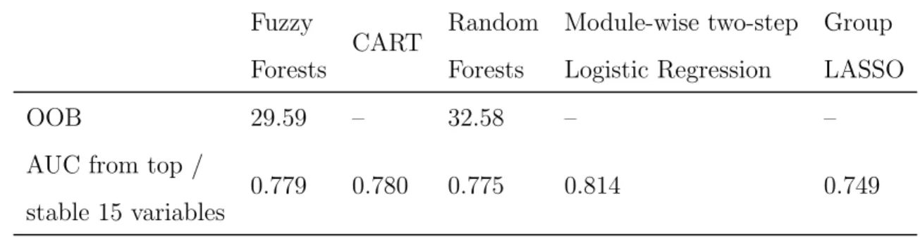
regression model and from a semi-parametric group LASSO procedure. Within each ap-proach, the 15 most important variables (out of 210) related to re-arrests are identified. Due to quasi-complete separation in the data when all of the predictors were considered simul-taneously, logistic regression was implemented using a stepwise procedure within modules identified by the Fuzzy Forests procedure. Area under the curve (AUC), which can be in-terpreted as the probability of correct ranking, along with the misclassification rate are two objective measures that are used to compare the performances of these methods.
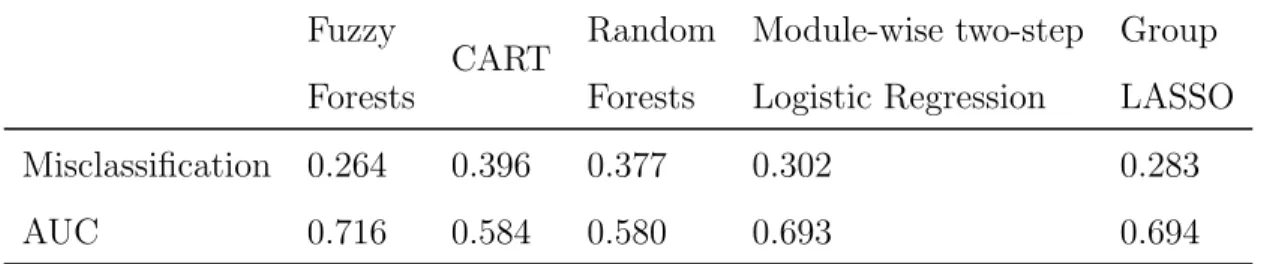
Results: The five methods identified several common variables in their list of the 15 most important variables for re-arrest. The resulting models applied to a hold-out sample indicate that Fuzzy Forests has the lowest misclassification rate and the highest AUC out of these five methods.
Conclusion: Machine learning methods can be very useful in studies with large number of variables by efficient dimension reduction, thereby facilitating comprehensive predictive modeling. A new method called Fuzzy Forests is useful when some of the explanatory vari-ables are correlated, as is likely among items within an instrument such as the CES-D. We found that Random Forests, Fuzzy Forests, CART, and stepwise logistic regression within