Confidence in classification: a Bayesian approach
Wojtek J. Krzanowski, Jonathan E. Fieldsend, Trevor C. Bailey,Richard M. Everson, Derek Partridge, and Vitaly Schetinin School of Engineering, Computer Science and Mathematics,
University of Exeter, Exeter, U.K.
Abstract
Bayesian classification is currently of considerable interest. It provides a strategy for eliminating the uncertainty associated with a particular choice of classifier-model parame-ters, and is the optimal decision-theoretic choice under certain circumstances when there is no single “true” classifier for a given data set. Modern computing capabilities can easily sup-port the Markov chain Monte Carlo sampling that is necessary to carry out the calculations involved, but the information available in these samples is not at present being fully utilised. We show how it can be allied to known results concerning the “reject option” in order to produce an assessment of the confidence that can be ascribed to particular classifications, and how these confidence measures can be used to compare the performances of classifiers. Incorporating these confidence measures can alter the apparent ranking of classifiers as given by straightforward success or error rates. Several possible methods for obtaining confidence assessments are described, and compared on a range of data sets using the Bayesian proba-bilistic nearest-neighbour classifier.
Keywords.
Accuracy-rejection plots; Bayesian classification; confidence measures; MCMC sampling; nearest-neighbour classifiers.
1
Introduction
Bayesian methods have been advocated in principle for many years (Lindley, 1965; DeGroot, 1970), but their application has been hampered in practice by the computational intractability of many of the concomitant (high-dimensional) integrals. This state of affairs has been revolu-tionised in recent years by the development of Markov Chain Monte Carlo (MCMC) methods (see, e.g., the review by Brooks, 1998) and their reversible-jump (RJ) extensions (Green, 1995). These methods allow samples to be drawn from posterior distributions that are known only up to a constant of proportionality, thereby sidestepping the evaluation of the difficult integrals and replacing other integrals by straightforward averages (or related simple summary statistics) of sampled values. The sampling process must usually be run for a very long time to allow the generated Markov Chains to stabilise at the required stationary distributions, but current
computing power makes light of this demand. Consequently, there has been an explosion in the use of RJMCMC methods for statistical modelling in the past ten years.
One specific area of interest in such methods is that of discriminant analysis, or supervised classification. In essence here the problem is to define a suitable function of p features x = (x1, x2, . . . , xp) that will best distinguish betweenga-priorigroups or populations, and that can be used to classify future unidentified individuals most accurately to their correct population. A set of individuals with known population membership is generally available for deriving the function (usually termed the classifier) and assessing its performance. If this set is large enough then it can be split into two independent parts to deal with these two aspects, the first part for training the classifier and the second part for testing its efficacy, but if the set is not large then some form of data resampling (such as jackknifing or bootstrapping) must be employed for the performance assessment. This whole area has now been studied for many years and there are many possible ways of deriving classifiers and determining their efficacies (McLachlan, 1992; Hand, 1997). A full Bayesian approach has only recently become viable, for the reasons outlined above, but the appropriate technology has been rapidly developed (Denison, Holmes, Mallick and Smith, 2002).
However, although the derivation of classifiers and the estimation of their classification per-formance has been worked out for a range of possible models and classifier types, other important aspects have received less attention. One such aspect, namely the confidence that can be ascribed to a particular classification result, is important in general but especially so in safety-critical systems such as medical diagnosis or air-traffic collision alert systems. We therefore focus in this paper on methods for deriving confidence measures about classifications in a Bayesian context. In section 2 we summarise the main features of Bayesian classification, in section 3 we derive several possible confidence measures and compare them on a range of data sets for one particu-lar classifier family, in section 4 we discuss how these measures can be used to choose between competing classifiers, and some concluding remarks are made in section 5.
2
Bayesian Classification
We first assume that the classifier C(x, θ) comes from a family of classifiers depending on the predictorsxas well as on a set of parametersθ = (θ0, θ1, . . . , θq). For example, a linear classifier belongs to the family C(x, θ) = θ0+θ1x1+θ2x2+. . .+θpxp of all linear combinations of the predictors, with coefficients and constant term comprising the set of parameters. Applying
the classifier to an individual x yields the values of one or more classification scores on which the classification of x is made; frequently these scores are the posterior probabilities of group memberships for x. However, in general θ is unknown and must be inferred from a set of individuals whose group memberships as well as predictor values are known. The classical single-classifier approach splits this set of individuals into atraining setD, say, and atest setT, say. Then θ is replaced by an estimate derived from D, and the resulting classifier’s efficacy is assessed by finding the proportion of each group that is misclassified inT. Different methods of estimation make different demands on the data; a common framework involves the assumption of a probability model for the dataD, and hence the use of maximum likelihood as the method of estimation.
Within such a framework, parametric probability models are frequently used for the popu-lations from which the groups are taken. In this case the classifier parametersθare functions of the population model parameters. For example, the earliest linear classifier between two popula-tions was derived empirically by Fisher (1936) and was subsequently formalised by Welch (1939), who modelled the two populations as two multivariate normal distributions having means µ1, µ2 and a common dispersion matrixΣ. The coefficientsθi in the linear classifier are then easily
shown to be functions of µ1, µ2 and Σ. In practice these unknown parameters are replaced by their estimates from the training data D to yield what is commonly termed Fisher’s linear discriminant function (LDF). If this function is denoted by F(x), say, then classification of x depends on whetherF(x)≤tor not, for some thresholdt. This is an example of a classification score that is not an estimate of posterior probability of group membership of x. In other clas-sifiers, e.g. logistic discriminators (McLachlan, 1992), the classification score does yield such a probability estimate.
For a Bayesian approach we need additionally to specify a joint prior distribution π(θ) for the classifier parameters, form the likelihood L(D|θ) of the training data using the chosen probability model, and hence obtain the posterior distribution of the parameters,
π(θ|D) = π(θ)L(D|θ)
π(θ)L(D|θ)dθ.
The Bayesian classifier is then the expected value of C(x, θ) over this posterior distribution, i.e. C(x|D) = C(x, θ)π(θ|D)dθ. This is known as the predictive classification score. If the classification scores are the posterior probabilities of group membership then these predictive values are often denoted byp(y|x, D), wherey is the group label variable.
and posterior distributions are for the latter parameters and the Bayesian classifier is the ex-pected value ofC(x, θ) over this latter posterior distribution. For example, in the case of Fisher’s LDF and multivariate normal assumptions as above, Geisser (1982) shows that on taking the usual reference prior expressing ignorance about the parametersµ1,µ2 andΣ, viz.
π(µ1,µ2,Σ)∝ |Σ|−(p+1)/2,
then the posterior distribution of the parameters is a multivariatetdistribution, and the expec-tation of C(x, θ) over this distribution isF(x) +p(n1−n2)/2n1n2, wheren1, n2 are the group sample sizes in the training data D.
This example involving Fisher’s LDF and multivariate normal assumptions is relatively un-usual, in that analytical derivation of the expectation of C(x, θ) is possible. More usually, evaluating the above two integrals can be very difficult, particularly when the dimensionality of θ is large. However, from its definition the Bayesian classifier will obviously be well approx-imated by the mean of C(x, θ) over a large sample of independent observations from π(θ|D). MCMC will enable such a sample to be drawn without having to evaluate the integral in the denominator of π(θ|D). We just need to ensure that the MCMC acceptance probabilities are chosen so that π(θ|D) is the limiting (stationary) distribution, run the chain for a preliminary (burn-in) period to ensure stationarity has been reached, and then sample (say) every 7th value. This will produce approximate independence of observations, and consistency when estimating higher-order moments. Each value then yields a single observation fromπ(θ|D), so substituting them in turn intoC(x, θ) for the particularxto be classified and averaging the results produces the Bayesian classifier.
This is just an example of Bayesian averaging, which is used much more generally in modelling (Hoeting, Madigan, Raftery and Volinsky, 1999). Of course, the Bayesian approach does not preclude the choice of a single “best” classifier, as one can simply be selected from the set of classifiers generated by the sampling process; the classifier obtained from the “maximum a-posteriori” (MAP) value of θ would be an obvious choice. However, an averaged classifier not only usually produces better overall performance than the single MAP classifier, it is also the optimal decision-theoretic choice when there is no single “true” classifier that is being sought from among the family C(x, θ) (Denison et al, 2002, pp 28-29). So it is the most appropriate one to use in many practical cases. The Bayesian approach has now been implemented for many different families of classifiers, and details may be found, for example, in Denison et al(2002); we use the nearest neighbour family in the illustrations below.
3
Measures of Confidence
3.1 Introduction
An important consideration in many applications, particularly with critical systems such as when air traffic controllers attempt to screen potential aircraft collisions, is the need to attach a measure of confidence relating to any particular classification. Although much effort has been expended in the past on refining classifiers and developing methods of accurate assessment of their overall performance, the estimation of uncertainty in classification prediction has been relatively under-appreciated.
A traditional method of reducing the risk of misclassification is by means of thereject option
(surveyed in Fukunaga, 1990), whereby we do not automatically accept the outcome of the classifier for all points in the sample space, but hold back any points about whose classification we have doubts with the aim of handling these points subsequently by different procedures. If the resultant cost is less than the cost of wrong classification then such a procedure will improve classification reliability. We can label points x held back in this way as having UNSURE classification, and all other points as having SURE classification. Among the latter will be ones that are classified correctly and others that are classified incorrectly by the chosen classifier, so adopting such an approach will lead to three categories of points in a test set: those whose classification is SURE and CORRECT, those whose classification is SURE but INCORRECT, and those whose classification is UNSURE.
We will therefore consider methods that allow us to construct these categories for any chosen classifier. Clearly, there is a scale of “sureness” along along which points are categorised as SURE or UNSURE, and for convenience we will align this scale with a probability scale of 0 to 1 (so that, for example, there will be more UNSURE points at a value of sureness of 0.9 than at one of 0.6). The Bayesian MCMC mechanism gives a good framework for developing the methodology, because consistency or otherwise of classification outcomes among the different classifiers produced by the MCMC sample is an obvious way of judging the uncertainty of the classification. In the next section we consider a number of possible methods.
3.2 Methodology
If we adopt the reject option approach, we need to establish how points should be held back. Various possibilities have been mooted (see, e.g., Bishop, 1995), but Chow (1970) showed that theoretically the optimal rejection rule is to hold back x if its maximum posterior probability
of allocation to any group is less than a thresholdt. Different values of t will lead to different proportions of UNSURE points and will therefore correspond to different levels of the “sureness” scale.
In practice, of course, the posterior probabilities of allocation have to be estimated. If we use the Bayesian approach they are given by the values of p(y|x, D) for each possible setting of y, so x will be held back if maxy{p(y|x, D)} < t. Providing that the classifier is one that delivers posterior probabilities p(y|x,θ, D) as classifier scores, p(y|x, D) is just the expecta-tion of these probabilities over the posterior distribuexpecta-tion π(θ|D) and so is simply estimated by m1 mi=1p(y|x, θi, D) over the m MCMC samples. Choosing a value of t and applying the classifier to all the pointsxin the test set will identify the points to be classified and the points to be held back, thereby generating estimated probabilities of SURE CORRECT, SURE IN-CORRECT and UNSURE classifications for the given populations at the chosen value oft. We will call this procedure the standard reject method.
However, not all classifiers deliver a posterior probability but instead give a classification score C(x, θi) for each classifier making up the MCMC sample, so what should be done here? The obvious possibility is to classify each point in the test data by each of these individual classifiers, and any pointx that is classified to the same group by more than a proportion tof classifiers could be deemed a SURE classification at “sureness” levelt, otherwise the classification is UNSURE. Here we convert each classifier result into a discrete variable (group to which x is classified) and then obtain the average incidence in each category, so the result can still be formally viewed as a posterior probability of allocation and hence falls within the scope of Chow’s result. In effect, if C(x, θi) = y indicates that the ith classifier allocates x to class y, then we are estimating p(y|x, D) by m1 mi=1I(C(x, θi) =y) where I(A) is the indicator function taking value 1 if A is true and 0 if A is false. In the feature space, this method produces a gradually widening envelope of classifications labelled UNSURE astincreases, so we will call it the envelope method.
Note that the envelope method uses consistency of actual classifications, so only labels points as UNSURE if they are unreliable in their classification rather than simply if their posterior probabilities of group membership are not high. It might therefore be a useful competitor to the standard reject method even when the classifier returns a posterior probability rather than just a classification score. However, it is important to see that the two methods deliverdifferent
estimates: the standard reject method estimates the expected value ofp(yi|x, θi, D) for specified class yi over the posterior distribution of the parameters π(θ|D), while the envelope method
estimates the expected value of the tail-area p(y = yi|x, θi, D) > p(y =yj|x, θi, D) ∀ j = i
over the same posterior distribution. The distinction is perhaps clearer in the two-class situation, where we need only look at the probabilities associated with one of the classes,y say. Then the comparison is between the posterior mean ofp(y|x, θi, D), i.e. the predictive distribution of the classification probabilities, and the posterior mean of I(p(y|x, θi, D) >0.5), i.e. the predictive distribution of the classification outcomes.
While there are some very specific situations when these have the same value (e.g. if
p(y|x, θi, D) is approximately constant overθand the posterior distribution is symmetric about 0.5), in general they will be different. We can demonstrate this, and highlight the points of difference in the two approaches, with a very simple example. Suppose that the classification probability p of the datum x to group y is given by a normal distribution with mean 0.6 and variance 0.01 (i.e. standard deviation 0.1), irrespective of the classification parameter values θ. In this case the posterior distribution of these parameters is immaterial, and the MCMC process simply delivers a stream of independent valuespifrom aN(0.6,0.01) distribution. By the strong law of large numbers the mean of this stream converges to 0.6 as the number of values tends to infinity, so the standard reject method delivers an estimated classification probability close to 0.6. By contrast, in the envelope method the value of eachpi is replaced by 1 if it exceeds 0.5 and by 0 otherwise. Thus, the probability that it is replaced by 1 equals the probability that a standard normal deviate exceeds 0.50−.10.6 =−1, which from normal tables equals 0.841. So by the strong law of large numbers again, the average of the 0/1 transformed pi values converges to 0.841 as the number of values tends to infinity. Thus the envelope method delivers an esti-mated classification probability close to 0.841, very different from the standard reject estimate (irrespective of for how long the MCMC process is run).
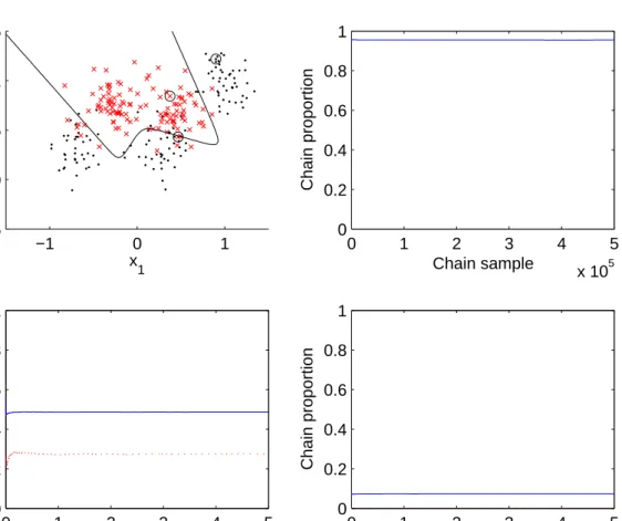
As a practical illustration of the differences, consider a synthetic two-class data set devised by Ripley (1994) and augmented with a further Gaussian function: it thus comprises five Gaussian components, 3 contributing to one class and 2 to the other (full details are given in Fieldsend
et al, 2003). The probabilistick−nearest neighbour classifier described in section 3.3 below was
applied to this data set, and the above two estimates were obtained for three data pointsx. The picture in the top-left corner of Figure 1 shows the data set, with the two classes denoted by circles and crosses respectively and the 0.5 Bayes classification probability contour marked. The three chosen points are highlighted: one is firmly in class 2, one is on the border between the classes, and one is in class 1. The other pictures in Figure 1 then show the two estimates of class 2 probabilities for each point (solid line for standard reject method, broken line for envelope
method) as a function of the number of MCMC samples collected, up to 5×10⁵ samples. The bottom left plot refers to the point on the decision boundary, where the reject estimate settles at about 0.5 while the envelope method settles at around 0.3. The other two plots refer to the points firmly in the two classes; here the envelope values stabilise at close 1 and 0 respectively, while the reject values are around 0.05 different from them.
Figure 1 about here.
Of course, the above two methods are not the only possible bases for estimation of uncer-tainty. A complete Bayesian summary would be to report the full conditional distribution of thep(y|x, θi, D), and to determine the categorisation ofxas SURE or UNSURE depending on the degree of overlap of these posterior distributions over groups. This introduces significantly greater computational effort, particularly if degree of overlap requires calculations of percentiles (and hence rankings of large amounts of data). Summary statistics of these posterior distri-butions would provide a first approximation. One possibility is to report a standard deviation as well as a mean, and then to base membership of the SURE category on whether or not the mean plus or minus a suitable multiple of the standard deviation exceeded the requisite threshold. We will call this the posterior distribution method; note, however, that this method carries an implication of symmetry of posterior distributions which may not be tenable. Another possibility is to compute m1 mi=1I(p(y|x, θi, D)> t), which estimates the posterior probability that p(y|x, θi, D) > t so we could label a point as UNSURE if this estimated probability fell below a thresholds. However, the point may be consistently and correctly classified even when
p(y|x, θi, D) exceeds t on very few occasions, so this criterion may be unnecessarily stringent. Moreover, the major drawback of all these suggestions is that they require the classifier to deliver posterior probabilities. We give some examples of the posterior distribution method below, but concentrate essentially on the standard reject and envelope methods in the main development.
It is also worth noting some connections between the above methods and other (non-Bayesian) multiple classifier systems. It has long been recognised that classification accuracy can be improved if a selection of diverse classifiers is employed, and a consensus view among them is taken when classifying x. One possible consensus is the average posterior probability of class membership ofx, which relates to the standard reject method, while another is the major-ity vote among the separate clssifications of x, which relates to the envelope method. Among majority vote strategies is the idea of “boosting”, which is essentially a weighted system with higher weights accorded to those classifications that have greater probabilities, and this is even
more closely linked to the MCMC scheme. For a recent discussion of all these ideas, together with relevant references, see Kuncheva (2004).
3.3 Applications
In order to conduct empirical investigations, we must first choose a family of classifiers. Many choices are possible, but to maintain flexibility while keeping the parameter dimensionality low we focus on k−nearest neighbour classifiers. To classify an observation x = (x1, . . . , xp) into one of ggroupsy = (1, . . . , g) using the standard (classical) k−nearest neighbour classifier, we:
1. define a metric in thex−space (usually Euclidean distance); 2. find the ktraining set members closest to x;
3. classifyx to the majority group among thesek.
The value of k can either be set by the user or chosen from D by some data-based procedure, e.g. cross-validation.
Holmes & Adams (2002) have given a probabilistic formulation of this process, and this enables a Bayesian approach to be taken. They define the likelihood of the data given parameters
kand β to be L(D|β, k) = n i=1 exp(aijiβ/k) jexp(aijβ/k),
whereaij is the number of theknearest neighbours to theith observation that belong to group
jandjiis the group to which theith observation belongs. Herekis the number of neighbours as above, andβ reflects the influence of neighbours on the group probabilities: the greater the value of β, the higher the probability of belonging to the group that has the majority of neighbours. By assuming some temporal ordering of the data points, Holmes and Adams (2002) then deduce the predictive distribution for the response at a new pointxas
p(y=i|x, β, k) = exp(aiβ/k)
iexp(aiβ/k),
whereai is the number of groupiindividuals among thek nearest training set neighbours ofx (i= 1, . . . , g), so that ai/k is the proportion of such individuals. Thus the predictive scores are given by
p(y=j|x, D) =
p(y=j|x, β, k)π(k, β|D)dkdβ,
Table 1: Data set details and overall classification performances
Data Set p D T % correct
Pima 8 512 256 77.1
Synthetic 2 250 1000 88.6
Sonar 60 138 70 87.1
Ionosphere 33 200 151 94.7 Wisconsin 9 455 228 99.6
We thus need to formulate a prior distribution π(k, β) for the two parameters. In the case of prior ignorance it is suggested that π(k, β) = π(k)π(β) where π(k) is a uniform distribution between 1 and min(n,200) and π(β) is a half-normal distribution (i.e. distribution of |x|when
x is normal) with large variance. Using a symmetric MCMC proposal, any proposed move to a new classifier from the current parameter settings (β, k) to new settings (β, k) is accepted ifu, a draw from aU[0,1] distribution, is less than min
1,LL(D(D|β|β,k,k))ππ((ββ,k,k))
, and otherwise the current values ofβ andkare retained. In all MCMC runs reported in this paper we used 10,000 burn-in and 10,000 post burn-in samples, the latter taken at a sampling rate of one in seven. Thus a total of 10,000 + 70,000 = 80,000 members constituted each chain, and graphical methods were used to verify that each chain had reached a stationary distribution by the end of its burn-in period.
We now apply both the standard reject and the envelope methods to a number of data sets. In order to avoid uncertainty over the lower bound of the threshold t in the reject method for multi-class data, where there are many ways in which posterior probabilities can be distributed among the classes, we consider only two-class sets here and so a lower bound for tis 0.5. One of these sets is the synthetic data described above, while the other four sets are from the UCI Machine Learning Repository; they are the Wisconsin, Ionosphere, Pima, and Sonar data sets respectively. The data-set details are given in Table 1 (number of predictors,p; size of training set, D; size of test set,T). Also shown in the table are the overall classification performances, i.e. the percent correct classification of the test set, for each data set.
To compare the envelope and reject methods we need to compare the proportions each method assigns to the three categories SURE CORRECT (SC), SURE INCORRECT (SI) and UNSURE (U). In order to do this we have found the proportions assigned to each of the three categories by the envelope method at each of three commonly used threshold values (0.80, 0.95 and 0.99). To standardise the two methods we have then found the assignments to the three categories for which the reject method gives the same SI proportion as the envelope method
(apart from the Pima 95% region where we standardised on the SC proportions), together with the reject threshold value that achieves this assignment. In a couple of cases there was a range of such values, and in these cases we have quoted the highest value in the range. We used the same MCMC output on both methods. All the results are given in Table 2 for each of the five data sets.
We also include the posterior distribution method for comparison with these data sets, since the probabilistic k−nearest neighbour classifier delivers posterior probabilities. To standardise
this method with the others we found the multiple of the posterior standard deviation that was needed in order to produce the same SC value as the envelope method, and where there were several possible multiples we chose the one that delivered a threshold value closest to the envelope value. These multiples are given in the column headed “s.d.”in Table 2.
In terms of proportions within each category (SC, U, SI), the envelope and standard reject methods of region construction give very comparable results (although the chosen probability thresholds are rather different). Where values differ between the two methods for a category, the better (i.e. lower SI or higher SC) value is shown in bold. We see that if we require strong consistency of classification (99% envelopes) then success rates (SC) show a fall from the unconditional rates in Table 1, but if we are prepared to tolerate weaker consistency then there is generally a closer match between the rates. Comparing the posterior distribution method with the envelope approach, the UNSURE proportions for the former are either equal to or greater than those for the latter in nearly all cases− but the differences are very small so the methods are very similar when posterior probabilities are produced by the classifier.
One way in which we could reduce the set of values to a single one for each method would be to assign a loss to each outcome (e.g. +2 for sure incorrect, 0 for unsure and−1 for sure correct) and to compare the expected loss across methods. The problem here is that in the absence of substantive knowledge of the particular classification task there is no guidance about suitable loss assignments; many arbitrary choices could be made, resulting in a plethora of comparisons, so we do not pursue this avenue here.
4
Choosing Between Classifiers
4.1 Methodology
Traditionally, classifier system performance has been measured simply by the percentage of test-set allocations that are correct (or by its complement, the error rate, or some simple variant
T a b le 2 : 80% , 95% an d 99% en v elop e m eth o d re gion s p lu s b es t m atc h in g rej ect m eth o d re gion s a n d b es t m a tc h in g p o st er ior d is tr ib u tion re gion s for fi v e d ata sets E n v elop e R egion s Re je ct Re g io n s P o ster ior D istr ib u tion Data # SC U SI # SC U SI s.d. SC U SI 80% 0.7656 0.0260 0.2083 51% 0.7656 0.0260 0.2083 2.0 0.7656 0.0417 0.1927 Pima 95% 0.7552 0.0521 0.1927 53% 0.7552 0.0469 0.1979 2.5 0.7551 0.0521 0.1927 99% 0.7448 0.0677 0.1875 54% 0.7552 0.0573 0.1875 4.0 0.7448 0.0833 0.1719 80% 0.8780 0.0160 0.1060 54% 0.8760 0.0180 0.1060 1.5 0.8780 0.0170 0.1050 Sy n the ti c 95% 0.8740 0.0270 0.0990 57% 0.8710 0.0300 0.0990 2.4 0.8740 0.0240 0.1020 99% 0.8700 0.0320 0.0980 57% 0.8680 0.0340 0.0980 4.0 0.8700 0.0360 0.0940 80% 0.8429 0.0286 0.1286 51% 0.8429 0.0286 0.1286 1.5 0.8429 0.0286 0.1286 So na r 95% 0.8286 0.0429 0.1286 51% 0.8429 0.0286 0.1286 2.0 0.8286 0.0429 0.1286 99% 0.8000 0.0857 0.1143 52% 0.8429 0.0429 0.1143 5.0 0.8000 0.0857 0.1143 80% 0.9470 0.0066 0.0464 51% 0.9470 0.0066 0.0464 1.5 0.9470 0.0066 0.0466 Io no sphe re 95% 0.9470 0.0066 0.0464 51% 0.9470 0.0066 0.0464 2.0 0.9470 0.0066 0.0466 99% 0.9338 0.0199 0.0464 51% 0.9470 0.0066 0.0464 4.0 0.9338 0.0265 0.0397 80% 0.9781 0.000 0.0219 93% 0.9781 0.000 0.0219 1.5 0.9781 0.000 0.0219 W isc o n sin 95% 0.9781 0.000 0.0219 93% 0.9781 0.000 0.0219 2.0 0.9781 0.000 0.0219 99% 0.9781 0.000 0.0219 93% 0.9781 0.000 0.0219 4.0 0.9781 0.000 0.0219
depending on problem-specific variation in the importance of the alternative classifications). Thus whenever a choice has to be made between competing classifiers, either the success rate or the error rate is the criterion on which the decision is based. Within a Bayesian approach to classification, the problem is generally turned into one of model choice and then the optimal model can be chosen on the basis of a criterion such as BIC (Schwarz, 1978). A good example is provided by Lee (2001), who uses this criterion for developing a procedure for model choice in neural network classification. But these statistics carry no information regarding the confidence with which the various classifications have been made. We have argued above for the use of SURE CORRECT, SURE INCORRECT and UNSURE as measures of confidence in classifications, so a better comparison between classifiers should be based on simultaneous use of all these measures. To see how this can be implemented, we draw on the work that has been done in classi-fier acceptance-reject rates (see, e.g., Giacinto, Roli and Bruzzone, 2000, for a summary). In particular, Battiti and Cola (1994) have shown that to compare the performance of different classifiers we need to compare their accuracies over a range of different rejection rates (i.e. dif-ferent threshold valuest), and this can be done by plotting these values in the accuracy-rejection (A-R) plane. In our case the UNSURE proportions at differenttvalues correspond to the rejec-tion rates, while “accuracy” is reflected by either of the SURE categories. We prefer to minimise SURE INCORRECT rather than maximise SURE CORRECT, so to compare different classi-fiers on a data set we compare the curves each produces when SURE INCORRECT is plotted against UNSURE for a range of values of t. The classifier corresponding to the lowest curve on such a plot is the one to be chosen.
4.2 Applications
To illustrate this methodology, we first need a set of classifiers to compare. There is an almost unlimited choice available to us, but to keep within a traditional statistical modelling framework we define a nested set ofk−nearest neighbour classifiers by providing first a simplification and then a generalization of the probabilistic classifier introduced above.
The simplified version is obtained by keeping β fixed at 1.0 throughout, and only sampling over k. Here the probability of x belonging to a particular group is directly proportional to the preponderance of this group among the k nearest neighbours of x, and there is thus no possibility of skewing this probability as the balance of neighbours between groups varies. We call this version the “simple” classifier as opposed to the other “standard” one.
of parameters to reflect scaling and rotation of the variables. This is equivalent to replacing the Euclidean metric d(x1,x2) = {(x1 −x2)t(x1−x2)}1/2 in step 1 of the k−nearest neighbour process by an “adaptive” metric d(x1,x2) = {(x1 −x2)tM(x1−x2)}1/2 where the (positive-definite) matrix M is chosen to optimise the classification with regard to differential scales and orientations of the variables. Various ways can be devised for achieving such an adaptive classifier (see, e.g., Myles and Hand, 1990, or Hastie and Tibshirani, 1996). Our approach is to take M = QΛQt, where Λ is a diagonal scaling matrix and Q = exp(S) with S a skew-symmetric rotation matrix. The proposals are generated by forming M =QΛQt, where quantities ri drawn independently from N(0,0.22) are added to the diagonal elements of Λ to give Λ, and Q = exp(S) where quantities si are drawn independently from N(0,0.12) and added to elements of S to give S. Further details are given by Everson and Fieldsend (2004); we call this version the “adaptive” classifier.
It is evident that the three classifier versions are therefore nested, with the simple one being a special case of the standard one and this in turn being a special case of the adaptive one.
4.2.1 Comparison of envelope and reject methods
To make this comparison as simply and directly as possible, we compare the two methods on just the simple Bayesiank−nearest neighbour classifier (i.e. only one parameterk) and the standard Bayesiank−nearest neighbour classifier (i.e. two parameterskandβ) on the five data sets used above; Figure 2 shows the accuracy-rejection plots for these data sets. The plots obtained using the envelope method are on the left, and those using the reject method are on the right; the curve obtained from the simple classifier is indicated by crosses, that from the standard classifier by open circles.
Figure 2 about here.
The first obvious difference between the envelope plots and the reject method plots is that the latter stretch across the wholex−axis while the former generally stop about half-way across. This is because the envelope plots are determined by the proportion of MCMC classifiers that classify to each group, and in all data sets there will be at least some points for which all classifiers allocate to one group. Such points have posterior group allocation probabilities of 1.0 so can never be categorised as UNSURE whatever the threshold value of t − even if their estimated posterior probabilities of classification are not very high. The reject method plots, on the other hand, are based directly on these estimated posterior probabilities which rarely
approach 1.0 for any data points (which may, in itself, be a recommendation for this method to the Bayesian). Hence the range of possible UNSURE values is much greater for the reject method than for the envelope method, and this feature is borne out by the plots. Indeed for some envelope plots the range of UNSURE values is either very short or nonexistent (e.g. for the Wisconsin data). Reference back to Table 2 shows that for these data sets there are either no or very few UNSURE points at the highest threshold value, so there cannot be any such points at lower threshold values.
With that proviso, it is evident that the differences between the two methods of construction are very slight, and that they both give the same qualitative conclusions regarding the com-parison between the simple and the standardk−nearest neighbour classifiers. Since the simple classifier is nested within the standard one we would expect the latter to have better classifica-tion performance (as the simple classifier is crude and the training samples are large), and this is generally the case in our examples. For the Pima, Synthetic and Sonar data sets the curve for the standard classifier lies distinctly below that for the simple classifier (although there is a small reversal at the lowest UNSURE value of the Sonar data). In the cases of Ionosphere the two classifiers give indistinguishable performances, the two curves virtually coinciding over the range plotted, while the Wisconsin data (as already noted) has virtually no variability for either classifier.
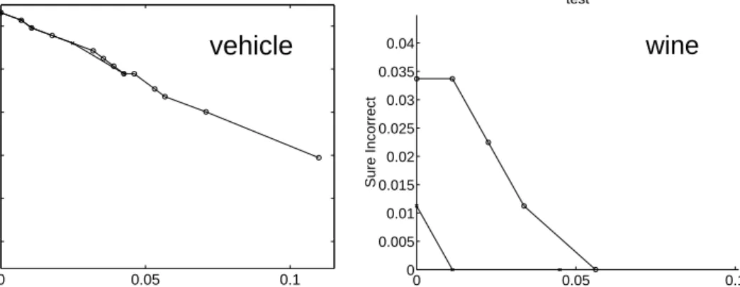
We have stressed earlier the ease of application of the envelope method to multi-class data, since the basic operation is no different from that in the two-class case. We therefore selected two more data sets from the UCI repository: the Wine data with 3 classes (p= 13, D= 89, T = 89, 96.6% correct classification) and the Vehicle data with 4 classes (p = 19, D = 564, T = 282, 67.4% correct classification). The accuracy-rejection plots for these sets are shown in Figure 3 for the envelope method.
Figure 3 about here.
The two classifiers give virtually indistinguishable performances for the vehicle data, the two curves lying more or less on top of each other, but for the wine data we have the apparently surprising result that the simple classifier has better performance than the standard classifier. However, this set of data is one with small data sets, relatively high number of variables and well-separated classes, so a difference of one or two classifications is enough to cause the result observed. We ran five separate MCMC chains and noted that the misclassification rates varied between 0% and 3.5% unpredictably across methods, so the apparent differences are well within
Table 3: Percentage of correct classifications in the test set for each classifier and each data set Classifier
Data Set simple standard adaptive
Pima 76.0 77.1 79.2 Synthetic 87.9 88.6 89.4 Sonar 85.7 87.1 84.3 Ionosphere 94.7 94.7 98.0 Wisconsin 99.6 99.6 98.7 Vehicle 63.8 67.4 77.0 Wine 98.9 96.6 98.9
the MCMC “noise” level for this data set.
4.2.2 Comparison of classifiers
We can now turn to comparison of the three versions of k−nearest neighbour classifier. First, we show in Table 3 the overall classification performances of each of these versions as judged by the percentage of correct classifications in the test setT of each data set.
Although there are one or two exceptions evident in the table, the broad trend of the results suggests that classifier accuracy improves on moving successively from simple to standard to adaptive, i.e. as the complexity of the k-nearest neighbour classifier increases. (Although the details are not shown here, the Bayesian-averaging classifier also generally gives better results than just the single-best MAP classifier.) However, we have argued above that such a way of judging classifier performance is too simplistic, and that we need to examine the SURE INCORRECT versus UNSURE plots of the classifiers over a range of values of t. In Figure 4 we therefore show these plots for the test data portion of each of the seven data sets. In each plot the simple classifier is indicated by crosses, the standard classifier by open circles, and the adaptive classifier by stars.
Figure 4 about here.
The picture now is less clear-cut than the error rate comparisons would suggest. The only data set in which the above trend is definitely supported is the Pima data, where the curve for the simple classifier lies completely above the curve for the standard classifier, and this in turn lies mostly above the curve for the adaptive classifier. Although the standard classifier curve is not completely above that for the adaptive classifier, it is nevertheless so for a sufficient part of the range of UNSURE values, so that we can indeed conclude that for this data set the adaptive
classifer is best, the standard classifier is next best, and the simple classifier is the poorest. We note that the test set for the Pima data is quite large (256 individuals).
The remaining data sets depart from the expected trend to a greater or lesser extent. Closest is the Synthetic data, where the simple classifier is uniformly the poorest again, but there is nothing to choose between the other two types. However, it is possible to establish the optimal Bayes error rate for Synthetic data; in this case both standard and adaptive versions are operating at close to the Bayes level, and such a large test set (1000 observations) permits accurate estimation of classification rates. For the Vehicle data there is in fact nothing to choose between all three types until near the very end of the range of UNSURE values, so by analogy with the Synthetic data result we infer that all three classifiers are operating at close to the Bayes level. We also note that the Vehicle test set is the second largest among our data sets (282 individuals). The Wisconsin data has very little variation across the whole range of classifiers, so can perhaps be discounted, while the Wine and Sonar data exhibit so many “cross-overs” of curves as to make any single conclusion meaningless. However, we note that these latter two data sets have very small test samples (89 and 70 respectively), so these “cross-overs” are a reflection of the large variability in small data sets. The one puzzling outcome is for the Ionosphere data, which show the reverse of the expected trend with the most complex classifier being the poorest until near the end of the UNSURE range. This result is opposite to the one suggested by consideration of the straightforward correct/incorrect dichotomy and would merit further investigation.
We therefore conclude from these experiments that although the addition of a confidence measure to the usual correct/incorrect assessment of classifiers is highly desirable, it carries a penalty in terms of sampling variability. The expected trends show up only generally when samples are large (particularly when test samples are large), and in small samples the picture is considerably less clear.
5
Conclusion
We have shown that Bayesian MCMC methodology can be allied to existing knowledge on the reject option in classification to produce a quantification of the confidence that can be ascribed to particular classification outcomes. One point that can be made here is that a typical Bayesian MCMC classification task gathers a vast amount of information, much of which is thrown away without further use. The envelope method makes use of some of this information;
it is very efficient in that it needs little more computation than is already carried out and has considerable added benefit, but nevertheless there is still information being thrown away by keeping only classifications rather than classification probabilities.
Of the two methods compared in detail, the envelope approach offers some direct advantages over the standard reject approach: interpretability in terms of familiar confidence coefficient ter-minology, guidance in choice of threshold values, and easy applicability to all types of grouping. It has been shown that incorporating confidence measures into a comparison of classifiers via the accuracy-rejection plots can make the comparison less clear-cut than the traditional one based solely on either success or error rates. This is related to the variability inherent in sample-based classifiers, which is often ignored when making error rate comparisons. A more realistic assessment might come from comparisons of confidence regions for error rates (see, e.g., Krzanowski, 2001), but this does not yet seem to be standard practice.
Indeed, it is surprising that classifier confidence has received so little attention, considering the emphasis placed on confidence regions in general statistical practice. The methods described here are easily built in to a standard Bayesian procedure so should be part of the general classification tool kit, especially in such areas as safety-critical applications. However, some aspects remain to be investigated. For example, what can be done if the available data are not extensive enough to be split into a training set D and a test set T? In a fully Bayesian approach, all data would be used without holding any out, and this would be accompanied by a formal model selection. The standard way of proceeding in the single-classifier frequentist case would be to use a data-based method of error rate estimation such as leave-one-out, but in our set-up each unit omission in effect creates a new set D for the MCMC process. So if such a scheme were to be contemplated then an efficient way of organising the computations would be essential. Similar considerations of efficiency are paramount if the variability of the results is to be established using, say, n−fold cross-validation on the (D, T) splits of the data.
While such aspects remain to be investigated, we nevertheless feel that use of the confidence measures described in this paper provide a distinct step forward in classifier technology.
Acknowledgement
This work has been supported by grant no. GR/R24357/01 of the Engineering and Physical Science Research Council. We thank the anonymous reviewers for their helpful comments, which have much improved our presentation.
References
BATTITI, R. and COLLA, A.M. (1994), “Democracy in neural nets: voting schemes for classi-fication,” Neural Networks, 7, 691-707.
BISHOP, C.M. (1995), Neural Networks for Pattern Recognition, Oxford: Clarendon Press.
BROOKS, S.P. (1998), “Markov chain Monte Carlo method and its application,” The Statisti-cian, 47, 69-100.
CHOW, C.K. (1970), “On optimum recognition error and reject tradeoff,” IEEE Transactions
on Information Theory, 16, 41-46.
DE GROOT, M.H. (1970), Optimal Statistical Decisions, McGraw-Hill.
DENISON, D.G.T., HOLMES, C.C., MALLICK, B.K. and SMITH, A.F.M. (2002), Bayesian
Methods for Nonlinear Classification and Regression, Chichester: John Wiley & Sons Ltd.
EVERSON, R.M. and FIELDSEND, J.E. (2004), “A variable metric probabilistic k−nearest neighbours classifier,”Proceedings of the Fifth International Conference on Intelligent Data
En-gineering and Automated Learning (IDEAL’04), Lecture Notes in Computer Science, vol 3177,
pp 659-664, Springer.
FIELDSEND, J.E., BAILEY, T.C., EVERSON, R.M., KRZANOWSKI, W.J., PARTRIDGE, D. and SCHETININ, V. (2003), “Bayesian inductively learned modules for safety critical sys-tems,”Proceedings of the 35th Syposium on the Interface: Computing Science and Statistics, pp 110-125, Salt Lake City.
FISHER, R.A. (1936), “The use of multiple measurements in taxonomic problems,” Annals
of Eugenics, 7, 179-184.
GEISSER, S. (1982), “Bayesian discrimination,” inHandbook of Statistics, Volume 2, Eds. P.R. Krishnaiah and L.N. Kanal, Amsterdam, North-Holland, 101-120.
GIACINTO, G., ROLI, F. and BRUZZONE, L. (2000), “Combination of neural and statistical algorithms for supervised classification of remote-sensing images,” Pattern Recognition Letters, 21, 385-397.
GREEN, P.J. (1995), “Reversible jump Markov chain Monte Carlo computation and Bayesian model determination,” Biometrika, 82, 711-732.
HAND, D.J. (1997), Construction and Assessment of Classification Rules, Chichester: John Wiley & Sons Ltd.
HASTIE, T. and TIBSHIRANI, R. (1996), “Discriminant adaptive nearest neighbor classifi-cation,” IEEE Transactions on Pattern Analysis and Machine Intelligence, 18, 607-616.
HOETING, J.A., MADIGAN, D., RAFTERY, A.E. and VOLINSKY, C.T. (1999), “Bayesian model averaging: a tutorial (with discussion),”Statistical Science, 14, 382-417.
HOLMES, C.C. and ADAMS, N. (2002), “A probabilistic nearest-neighbour method for sta-tistical pattern recognition,” Journal of the Royal Statistical Society Series B, 64, 1-12.
KRZANOWSKI, W.J. (2001), “Data-based interval estimation of classification error rates,”
Journal of Applied Statistics, 28, 585-595.
KUNCHEVA, L.I. (2004), Combining Pattern Classifiers, Methods and Algorithms, New Jer-sey: John Wiley & Sons Ltd.
LEE, H.K.H. (2001), “Model selection for neural network classification,” Journal of
Classifi-cation, 18, 227-243.
LINDLEY, D.V. (1965), Introduction to Probability and Statistics from a Bayesian Viewpoint.
MCLACHLAN, G.J. (1992), Discriminant Analysis and Statistical Pattern Recognition, New York: John Wiley & Sons Ltd.
MYLES, J.P. and HAND, D.J. (1990), “The multi-class metric problem in nearest neighbour discrimination rules,”Pattern Recognition, 23, 1291-1297.
RIPLEY, B.D. (1994), “Neural networks and related methods for classification (with discus-sion),” Journal of the Royal Statistical Society Series B, 56, 409-456.
SCHWARZ, G. (1978), “Estimating the dimension of a model,” Annals of Statistics, 6, 461-464.
0 1 2 3 4 5 x 10⁵ 0 0.2 0.4 0.6 0.8 1 Chain sample Chain proportion 0 1 2 3 4 5 x 10⁵ 0 0.2 0.4 0.6 0.8 1 Chain sample Chain proportion 0 1 2 3 4 5 x 10⁵ 0 0.2 0.4 0.6 0.8 1 Chain sample Chain proportion −1 0 1 −0.5 0 0.5 1 1.5 x 1 x 2
Figure 1: Synthetic data (top left), plus plots of the standard reject (solid line) and envelope (broken line) probability estimates of Pr(x∈class 2) across 5×10⁵ MCMC samples.
0 0.02 0.04 0.06 0.08 0.1 0.12 0.18 0.2 0.22 0.24 0.26 0.28 Unsure Sure Incorrect pima 0 0.02 0.04 0.06 0.08 0.1 0.12 0.18 0.2 0.22 0.24 0.26 0.28 Unsure Sure Incorrect pima 0 0.005 0.01 0.015 0.02 0.01 0.02 0.03 0.04 0.05 0.06 test Unsure Sure Incorrect wisconsin 0 0.005 0.01 0.015 0.02 0.01 0.02 0.03 0.04 0.05 0.06 test Unsure Sure Incorrect wisconsin 0 0.01 0.02 0.03 0.04 0.05 0.06 0.08 0.085 0.09 0.095 0.1 0.105 0.11 0.115 0.12 test Unsure Sure Incorrect synthetic 0 0.01 0.02 0.03 0.04 0.05 0.06 0.08 0.085 0.09 0.095 0.1 0.105 0.11 0.115 0.12 test Unsure Sure Incorrect synthetic 0 0.05 0.1 0.15 0.08 0.1 0.12 0.14 0.16 0.18 0.2 Unsure Sure Incorrect sonar 0 0.05 0.1 0.15 0.08 0.1 0.12 0.14 0.16 0.18 0.2 Unsure Sure Incorrect sonar 0 0.02 0.04 0.06 0.08 0.04 0.06 0.08 0.1 0.12 0.14 0.16 Unsure Sure Incorrect ionosphere 0 0.02 0.04 0.06 0.08 0.04 0.06 0.08 0.1 0.12 0.14 0.16 Unsure Sure Incorrect ionosphere
Figure 2: Accuracy-rejection plots for the 2-group data sets; envelope method on left, reject method on right, circles for general classifier and crosses for simple classifier.
0 0.05 0.1 0.22 0.24 0.26 0.28 0.3 0.32 Unsure Sure Incorrect
vehicle
0 0.05 0.1 0 0.005 0.01 0.015 0.02 0.025 0.03 0.035 0.04 test Unsure Sure Incorrectwine
Figure 3: Accuracy-rejection plots for the multi-group data sets using the envelope method; circles for the general classifier, crosses for the simple classifier.
0 0.005 0.01 0.015 0.02 0.01 0.02 0.03 0.04 0.05 0.06 test Unsure Sure Incorrect
wisconsin
0 0.05 0.1 0.22 0.24 0.26 0.28 0.3 0.32 Unsure Sure Incorrectvehicle
0 0.02 0.04 0.06 0.08 0.04 0.06 0.08 0.1 0.12 0.14 0.16 Unsure Sure Incorrectionosphere
0 0.05 0.1 0.15 0.08 0.1 0.12 0.14 0.16 0.18 0.2 Unsure Sure Incorrectsonar
0 0.01 0.02 0.03 0.04 0.05 0.06 0.08 0.085 0.09 0.095 0.1 0.105 0.11 0.115 0.12 test Unsure Sure Incorrectsynthetic
0 0.05 0.1 0 0.005 0.01 0.015 0.02 0.025 0.03 0.035 0.04 test Unsure Sure Incorrectwine
0 0.02 0.04 0.06 0.08 0.1 0.12 0.18 0.2 0.22 0.24 0.26 0.28 Unsure Sure Incorrectpima
Figure 4: Accuracy-rejection plots for all data sets using the envelope method; crosses for the simple classifier, circles for the general classifier, stars for the adaptive classifier.