Diversity Assessment in Many-Objective
Optimization
Handing Wang,
Member, IEEE,
Yaochu Jin,
Fellow, IEEE,
Xin Yao,
Fellow, IEEE,
Abstract—Maintaining diversity is one important aim of multi-objective optimization. However, diversity for many-multi-objective optimization problems is less straightforward to define than for multi-objective optimization problems. Inspired by measures for biodiversity, we propose a new diversity metric for many-objective optimization, which is an accumulation of the dis-similarity in the population, where an Lp-norm-based (p < 1) distance is adopted to measure the dissimilarity of solutions. Empirical results demonstrate our proposed metric can more accurately assess the diversity of solutions in various situations. We compare the diversity of the solutions obtained by four pop-ular many-objective evolutionary algorithms using the proposed diversity metric on a large number of benchmark problems with two to ten objectives. The behaviors of different diversity maintenance methodologies in those algorithms are discussed in depth based on the experimental results. Finally, we show that the proposed diversity measure can also be employed for enhancing diversity maintenance or reference set generation in many-objective optimization.
Index Terms—diversity, many-objective optimization, metric, evolutionary algorithm
I. INTRODUCTION
Many-objective optimization [1] has become an active research topic in multi-objective evolutionary algorithms (MOEAs) [2], because of the challenges it poses to evolution-ary algorithms and practicability in the real world [3], [4], [5], [6]. Many-objective optimization problems (MaOPs) [1], [7], i.e. multi-objective optimization problems (MOPs) [8] with more than three objectives, are hard to be solved by most existing MOEAs [9], [10].
None of the three main approaches, Pareto-, aggregation-and performance indicator-based MOEAs is able to efficiently produce a solution set for MaOPs with satisfactory conver-gence and diversity [9]. The failure of Pareto-based MOEAs to converge on MaOPs comes from their ineffectiveness in distinguishing the quality of solutions when the number of objectives becomes large [11], [12], which is completely different from their efficiency on MOPs with two or three
This work was supported by two EPSRC grants (No. EP/M017869/1 and No. EP/J017515/1), in part by the National Natural Science Foundation of China (Nos. 61271301, 61329302 and 61590922), and in part by the Joint Research Fund for Overseas Chinese, Hong Kong and Macao Scholars of the National Natural Science Foundation of China (No. 61428302). Xin Yao was supported by a Royal Society Wolfson Research Merit Award.
H. Wang is with the Department of Computer Science, University of Surrey, Guildford GU2 7XH, U.K. (e-mail: [email protected]).
Y. Jin is with the Department of Computer Science, University of Surrey, Guildford GU2 7XH, U.K. (e-mail: [email protected]). He is also affiliated with the State Key Laboratory of Synthetical Automation for Process Industries, Northeastern University, Shenyang, China.
X. Yao is with the School of Computer Science, University of Birmingham, Birmingham B15 2TT, U.K. (e-mail: [email protected]).
objectives (eg. NNIA [13]), even though the speed of the non-dominated sort for MaOPs has been improved by fast sorts [14], [15], [16], [17]. Aggregation-based MOEAs such as MOEA/D [18] decompose an MaOP into a number of single-objective optimization problems using a set of pre-defined weight vectors, thereby avoiding the convergence problem. However, a limited number of weight vectors in the high-dimensional space lead to poor diversity for MaOPs [19], [20]. Indicator-based MOEAs use an indicator as their fitness function to optimize an MaOP, which can be classified into three categories (distance-, hypervolume-, R2-based MOEAs) [10]. Iε+ [21] is the earliest distance-based indicator that
is used in IBEA to improve convergence, but it is not a diversity indicator and leads to poor diversity [12]. In contrast, hypervolume evaluates both convergence and diversity [22], thus many hypervolume-based MOEAs [23], [24], [25] have been developed. Although the computational complexity for calculating the exact hypervolume has been lowered [26], [27], MOEAs rely on on-line hypervolume calculation have not been applied to MaOPs [28]. R2 [29] evaluates both convergence and diversity and R2-based MOEAs for MaOPs have been reported in [30], [31].
Existing research on MaOPs can be roughly divided into four categories, objective reduction [32], [33], incorporation of preferences [34], modified dominance relationships, and introduction of additional selection criteria. In case there is a strong correlation between objectives, some objectives can be removed [35]. To this end, statistical machine techniques, such as feature selection [36], principal component analysis (PCA) [37], [38], and maximum variance unfolding (MVU) [39] can be employed for objective reduction. In practice, users are often interested in only a part of the Pareto optimal solutions [40]. Therefore, if user preferences are available, preference-based approaches can be designed [41], [34], [42], [43]. To improve the effectiveness in distinguishing solutions in many-objective optimization, several modified dominance relations [44], [45], [46], [47], [48] have been proposed. To accelerate the convergence of MOEAs (Pareto-, aggregation-and performance indicator-based) for solving MaOPs, addi-tional selection criteria have been introduced [49]. For ex-ample, NSGA-III [50] employs a set of reference points to maintain population diversity, where the reference points can be considered as a set of preferred solutions. Knee point driven evolutionary algorithms (KnEA) [51] uses the distance of knee points to a hyperplane as an additional selection criterion. Two Arch2 [52] adapts an Lp-norm distance-based selection criterion in addition to its Iε+-based selection. The
aggregation-based techniques.
It is well recognized that performance indicators of MOEAs should be able to account for convergence, diversity and uniformity of the solution set [22], [54], [55]. However, MaOPs may pose serious challenges to existing performance indicators in assessing convergence, diversity and uniformity. For instance, ratio-based performance indicators such as error ratio (ER) [56] and ratio of non-dominated individuals (RNI) [57], and binary performance indicators, including C-metric [58] and Purity [59], require dominance comparisons, which are less effective for MaOPs. In addition, distance-based performance indicators, e.g., maximum Pareto front error (MPFE) [56], generational distance (GD) [56], and GDp[60] need to sample a large set of uniformly distributed reference points sampled from the true Pareto front, which is hard to guarantee for MaOPs. Note that some performance indicators are able to account for both convergence and diversity, such as hypervolume [22], R2 [29], inverted generational distance (IGD) [61], and averaged Hausdorff indicator∆p [62].
Unlike uniformity metrics such as distribution (UD) [57], spacing (SP) [63], and minimal SP [59], diversity is less straightforward to characterize mathematically. Existing di-versity metrics view didi-versity from different perspectives. For examples, maximum spread (MS) [58] uses the spread of a solution set, whereas both number of distinct choices (NDC) [64] and entropy-based metric suggested in [65] em-ploy divided grids in the objective space. By contrast, sigma diversity metric (SDM) [66] assigns several reference lines and diversity measure (DM) [67] adopts a reference set. In addition, there are some metrics that can assess both diversity and uniformity, such as ∆ [68] and diversity comparison indicator (DCI) [55]. However, the above-mentioned metrics may encounter difficulties in assessing diversity for MaOPs due to the following two reasons. First, spread will no longer be able to fully characterize the diversity of the whole Pareto front in a high-dimensional space. Second, parameters in the diversity metrics are harder to specify for MaOPs.
This paper aims to address the difficulties the existing diversity metrics encounter in many-objective optimization. We propose a new diversity metric inspired by a measure for biodiversity. We show that the proposed new diversity metric is able to more accurately measure the diversity of solutions in high-dimensional spaces. Furthermore, our results indicate that the proposed diversity metric can enhance the diversity performance of evolutionary algorithms for solving MaOPs replying on a pre-defined reference set or weight vectors.
The rest of this paper is organized as follows. The dif-ficulties in assessing diversity for MaOPs are discussed in Section II. To address these difficulties, Section III presents a new diversity metric, together with empirical comparative analysis of its ability to measure diversity and the influence of convergence on the diversity measure. In Section IV, we employ the proposed metric to assess the diversity perfor-mance of four popular MOEAs for MaOPs and discuss the theoretical rationale behind these empirical results. In Section V, the proposed diversity measure is adopted for maintaining diversity or generating a reference set, which is shown to be able to enhance the diversity of solutions obtained by the
MOEAs under comparison. Section VI concludes the paper. II. DIVERSITY INEVOLUTIONARYMULTI-OBJECTIVE
OPTIMIZATION
Diversity is an important topic in multi-objective optimiza-tion, which provides decision makers information for choosing preferred solutions. When clear user preferences are not avail-able, it is highly desirable that a limited number of solutions can be obtained that uniformly spread over the whole PF and are as diverse as possible. However, unlike convergence, a well established definition for diversity of solutions obtained by MOEAs still lacks.
Diversity and uniformity are two related aspects for e-valuating the distribution of an obtained solution set. More often than not, researchers are confused about the meanings of these two measures. It should be stressed that a solution set with good uniformity does not necessarily mean that it also has good diversity, and vice versa. Generally speaking, solutions in a set with good uniformity should have the same dissimilarity with their neighbors, whereas solutions in a set with good diversity should provide decision makers the maximum amount of information. Mathematically, diversity and uniformity can be described as in Equations (1) and (2), whereX is a solution set andsis a solution inX. It is worth noting that dissimilarity(s, X−s)is the dissimilarity of s
to the rest of X (or the diversity contribution to X), which measures the different degree ofsto other solutions inX. In the existing research, there are different metrics to describe the dissimilarity between solutions, such as various distances. Therefore, the sum of dissimilarity(s, X−s) indicates the diversity ofX, while the variance ofdissimilarity(s, X−s)
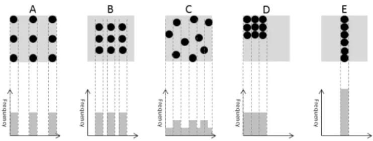
specifies the uniformity. diversity(X) =∑ s∈X dissimilarity(s, X−s) (1) unifomity(X) = var s∈X (dissimilarity(s, X−s)) (2) In order to better understand Equations (1) and (2), we use Fig. 1 to illustrate the differences between diversity and uniformity. Solution sets in panels A, B, D and E of the figure show good uniformity but relatively poor diversity. Solutions in panels D and E are of obviously poor diversity, because they are distributed only in small parts of the whole PF. Solutions in panel B loses information of the boundary of the PF. Although solutions in panel A are distributed over the whole PF with perfect uniformity, there is redundancy in the information on each objective, resulting in worse diversity than those in panel C. From these examples, we can see that a solution set with good diversity means that it contains the maximum amount of information for decision makers.
A. Challenges in Diversity Assessment for MaOPs
The high-dimensional objective space in MaOPs does not only make it very hard for decision makers to intuitively judge the diversity of the solution set, but also creates difficulties in quantitatively assessing the diversity. As we know, a solution
Fig. 1. Illustration of the differences between diversity and uniformity.
set of a limited size can distribute only very sparsely in a high-dimensional space [69], which is known as “curse of dimensionality”. In other words, a solution set of a limited size is hard to describe a PF in high dimensions, which causes trouble to decision makers in solving MaOPs. Therefore, diversity maintenance and assessment pose a serious challenge to many-objective optimization.
B. Existing Diversity Metrics
Existing diversity metrics can be divided into two classes, mixed and unmixed diversity metrics. Unmixed metrics mea-sure the diversity only, but mixed metrics try to capture more aspects of the distribution of a solution set (convergence for instance).
Table I provides a summary of widely used existing diversity metrics.
TABLE I
EXISTING DIVERSITY METRICS AND THEIR CHARACTERISTICS. Metric Mixed Parameter Needed Reference Needed
MS [58] N N N NDC [64] N Y N Entropy [65] N Y N SDM [66] N Y Y DM [67] N Y Y ∆[68] Y N N DCI [55] Y Y N Hypervolume [22] Y N Y IGD [61] Y N Y R2 [29] Y N Y ∆p[62] Y N Y
The first five metrics are unmixed, which can characterize diversity only, and their disadvantages are obvious. MS [58] uses the spread of a solution set as a measure of diversity, which is incomplete to evaluate the diversity of the whole solution set. NDC [64] and Entropy [65] divide the objective space into a number of grids (b divisions for each objective), NDC counts the number of grids having solutions in them and Entropy calculates the entropy of all the non-empty grids. They both require a pre-determined parameterb, which greatly affects the assessment result. SDM [66] assigns several reference lines to determine whether solutions are located near the lines by a distance thresholdd, thus the diversity based on reference lines can be obtained. DM [67] uses the projection of the solution set to reference (m-1)-dimensional grids for measuring diversity, which requires both the number of grids and the reference set.
The rest six metrics are unmixed, which evaluate more than diversity. Consequently, it is hard to single out the performance on diversity only from the value of these metrics.∆ assesses the distribution of the solution set [68].∆is a combination of the spread (measured by distances to the extreme points) and uniformity (measured by distances to the nearest neighbors). DCI [55] also employs a grid environment to assess both spread and uniformity, so the number of grids needs to be pre-defined. Hypervolume calculates the volume that the obtained solution set dominates respect to a reference point [70], but it cannot be applied to MaOPs in practice due to its prohibitively high computational complexity [27]. IGD is the average distance from a reference set (samplings on the true PF) to the obtained set. The idea of R2 is similar to IGD, where the reference set used is a set of weights, and the distance from the reference set to the solutions is calculated using the Tchebycheff function.∆p is the Hausdorff distance between the obtained solution set and the reference, which evaluates both convergence and diversity and has been applied to both MOPs [71], [72] and MaOPs [73]. However, a reference set is still needed to calculate ∆p.
Ideally, a diversity metric should assess diversity only and should be independent of any parameters or references. The main reason is that parameters or references may reduce the level of objectivity. Unfortunately, none of the existing diversity metrics fully satisfy the above requirements.
III. PROPOSEDPUREDIVERSITYMETRIC
A widely accepted definition for diversity still lacks in the area of evolutionary multi-objective optimization. By contrast, measures for biodiversity has been extensively studied in biology. Among various measures for biodiversity, the pure diversity has been proposed for measuring the diversity of species [74] as follows. PD(X) =max si∈X (PD(X−si) +d(si, X−si)) (3) where, d(s, X) =min si∈X (dissimilarity(s, si)). (4) In the above equations, d(si, X−si) denotes the dissimi-laritydfrom one speciessi to a communityX.
We can find that Equations (3) and (1) are equivalent except for the difference in the defining the sum, if s is viewed as a solution in the solution set X. In addition, Equation (3) does not require any reference, nor any parameters. Thus, pure diversity in Equation (3) can be a promising measure for population diversity in multi-objective optimization.
Fig.2 provides an illustrative example of how pure diversity is calculated. In the left panel of the figure, solution si and other solutions X −si are considered as two communities. Their diversity is the sum of diversity ofX−si (black dots) and the dissimilarity of si to X−si. With the recursion in Equation (3), the dissimilarity of every single solution to the whole population can be evaluated, with each solution being linked to its nearest unreplicated neighbor. Then, the sum of those dissimilarity results in the diversity of the whole
population, which can be seen as the structure ofX, as shown in panel B of Fig. 2 (where the darker lines are connected earlier than the lighter lines).
Fig. 2. Illustration of the pure diversity metric. A:d(si, X−si)is calculated
by the dissimilarity ofsito its nearest neighbor. B: the PD value ofXis the
sum of the linked dissimilarity.
To calculate the value of pure diversity (PD) of a population with n solutions, an n×n dissimilarity matrix D for every two solutions is needed. Details of the calculation of PD are given in Algorithm 1. In each accumulation, solution i with the maximal dissimilarity to its nearest unmarked neighbor
j is chosen by line 5, where d = min(D,[],2) means the smallest elements along the second dimension (the row of D). In order to avoid repeated choice ofi, we updateD(i,:)
to -1. Furthermore, any connected subgraph is avoided in PD, because a connected subgraph implies the dissimilarity of those solutions is repeatedly evaluated. When i and j
can be connected via previously assessed solutions, we let D(i, j) = Dmax and D(j, i) = Dmax, thus dissimilarity i and j cannot be used. If we skip line 8 in Algorithm 1, the connected subgraphs cannot be linked by other solutions, the dissimilarity from the subgraphs cannot be measured.
Algorithm 1 Pseudo code for the calculation of PD.
Input: D-dissimilarity matrix of every two solutions.
1: SetDmaxas the maximal element ofD.
2: Dmax=Dmax+ 1,P D= 0.
3: Set the diagonal elements ofD asDmax.
4: fork= 1 :n−1 do
5: d=min(D,[],2).//Find the nearest neighbor to each solution according toD in each row.
6: Find solutioniwith the maximaldi to its neighbor j.
7: while iand j is connected by previous assessed solu-tionsdo
8: D(i, j) =Dmax andD(j, i) =Dmax.// Mark the connected subgraph.
9: d=min(D,[],2).
10: Find solution i with the maximaldi to its neighbor
j.
11: end while
12: P D=P D+di.
13: D(i,:) =−1.//Mark the chosen solutioni.
14: D(j, i) =Dmax.// Mark the used dissimilaritydi.
15: end for Output: P D;
A. Dissimilarity
The evaluation of dissimilarity plays an important role in calculating PD. Usually, the distance between two solutions is adopted as their dissimilarity. Note however, that the Euclidean distance is not well suited for measuring neighborhood in a high-dimensional space [75], [76]. Since solutions of MaOPs are distributed in a high-dimensional objective space, the Euclidean distance (L2-norm-based) is not suited for
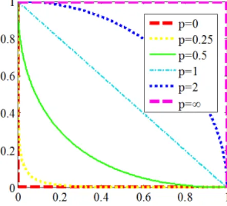
dissim-ilarity calculation in PD. To address this issue, Lp -norm-based distances have been suggested for diversity maintenance in solving MaOPs [76], [52], [77]. Fig. 3 illustrates the differences between variousLp-norm-based distances.
Fig. 3. Contour lines of different unit lengthLp-norm. The smallerpis, the
more sensitiveLpis to 0 in each dimension.
From Fig. 3 we can clearly see that the smaller p is, the more sensitive Lp is to 0 in each dimension. In contrast, the
Lp-norm-based distance measures are not good for measuring dissimilarity of high-dimensional data forp≥1. Therefore, it is necessary to setp < 1 for measuring diversity in MaOPs. It has been shown that the effectiveness of the measure is not sensitive to p as long as p < 1 [75]. Therefore, p is not a parameter in PD and we setpto 0.1 in this paper.
B. Behavior Study
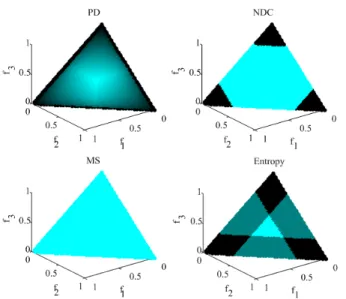
Indicators use a single scalar value to describe an m -dimensional distribution, thus some information will be lost no matter whichever indicator it is. Therefore, it is hoped that some key information is captured, although different indicators may capture different information. In the case that three extreme points of the PFf1+f2+f3= 1are obtained,
the values of diversity metrics vary with different solutions added to the set of three extreme points. Fig. 4 is the changing values of PD, MS, NDC (b= 4), and Entropy (b = 4) when another solution from the PF is added to the set of three extreme points, where the color shows the size of metrics (the darker points have lower values than the lighter ones). If one solution is selected based on those metrics to increase diversity, the lighter parts in Fig. 4 have priority over the darker parts. Once the extreme points have been obtained, the MS value reaches its maximum. Thus, no solution is able to improve MS anymore. Although the middle part is promoted by NDC and Entropy, solutions cannot be distinguished within
their grids. For PD, the middle part is promoted and the values change continuously. From Fig. 4, we find that PD can generally promote diverse solutions.
Fig. 4. Changing values of PD, MS, NDC (b= 4), and Entropy (b= 4) when another solution from the PFf1+f2+f3= 1is added to the set of
three extreme points, where the color shows the size of metrics (the darker points have lower values than the lighter ones).
To further understand PD, we calculate the PD values of six sets of solutions with different PF distributions (f1+f2+f3=
1) shown in Fig. 5, where red dots are solutions, lines are the dissimilarity accumulated in PD, and the colors of lines denote the chosen order (the darker lines are chosen earlier than the lighter lines). From Fig. 5, we can see that set A spread very well over the whole PF, while sets B, C, and D do not. Thus, the diversity of sets B, C and D should be worse than that of A, which is also reflected by the PD values.
Distinguishing sets A, E, and F from sets B, C, and D is the first step of PD, which comes from the aspect of spread. Further to spread to the whole PF, any repeated objective values are redundant to decision markers. Comparing A with E and F, we believe that A has better diversity than E and F, because A shows perfect uniformity. However, as the bar chart of the frequency of A shows, solutions in set A has many repeated objective values on f1, whereas E has no repeated
objective values on f1. Fig. 6 also shows that A has repeated
objective values onf1,f2, andf3, but E does not. Therefore,
E can provide more information to decision markers than A, which is therefore considered to have better diversity than A. The PD values of these solution sets indicate that it is able to detect the subtle differences in diversity between these solution sets.
So far we have revealed some promising properties of PD using illustrative examples. To further examine the usefulness of PD in diversity maintenance in many-objective optimiza-tion, we will perform a few additional experiments in the following, where we use an m-objective problem whose front can be characterized by∑mi=1fi= 1, as shown in Fig. 5. We use two different solution sets, one uniformly distributed set
U(n, m)denoted by A, and the other randomly distributed set
Fig. 5. Six different solution sets and their PD values.
R(n, m) denoted as E, where nis the size of the set and m
is the number of objectives.
To show the influence of the number of objectives on PD, we conduct the following experiments:
• Generate the test datasetR(100, m)for 30 times form= [2, ...,10], respectively.
• Calculate their PD values.
Fig. 7 shows the average values of PD on a randomly dis-tributed set with different numbers of objectives. Given a fixed number of solutions, the higher the dimension of the objective space, the more sparse the distribution of the solutions will be, the higher the degree of diversity will probably be. Therefore, MOEAs tend to achieve a set of solutions of a high degree of diversity but poor convergence [10]. Because of that poor balance of convergence and diversity, most MOEAs fail on many-objective optimization problems. That is the reason why the PD value increases dramatically with the increased number of objectives.
Fig. 7. Average PD values of a randomly distributed set with 100 solutions and different numbers of objectives.
To show the effects of spread on PD, we conduct the following experiment:
• Generate the test datasetR(100, m)for 30 times form= 3,10, respectively.
• Randomly remove different numbers of solutions in each dataset to change the spread, then calculate their PD values.
Fig. 8. Average PD values of randomly-distributed set with different numbers of dropped solutions for the 3 and 10-objective problems.
Fig. 8 shows the average PD values of randomly distributed sets with different numbers of solutions being removed for a 3- and 10-objective problems. As the number of solutions to
be removed increases, the PD value decreases on all the test datasets with different numbers of objectives. The results show that PD is able to detect diversity loss resulting from the loss of solutions.
Taking Fig. 9 as an example, when solution C is added to set A,B, the PD value increases due to the dissimilarity of A and C. However, when solution D is added to set A,B, the PD value is not improved, because there is no more dissimilarity added. Therefore, we find that the number of solutions is not directly related to PD. The PD value increases only if the additional solutions bring more dissimilarity to the solution set, which can be shown in Fig. 10. Even the set of 3 solutions can have a larger PD value than the set of 20 solutions, because the former spreads more widely than the latter.
Fig. 9. Example of the effect of the number of solutions on PD.
Fig. 10. PD values of two sets of 3 and 20 solutions.
To study the the impact of solutions having repeated objec-tive values on PD, we conduct the following experiments:
• Generate datasets U(n, m) andR(n, m) for m= 3,10, respectively, wheren=Cmq+q−1. For 3-objective and 10-objective problems,nequals 105 and 220, respectively.
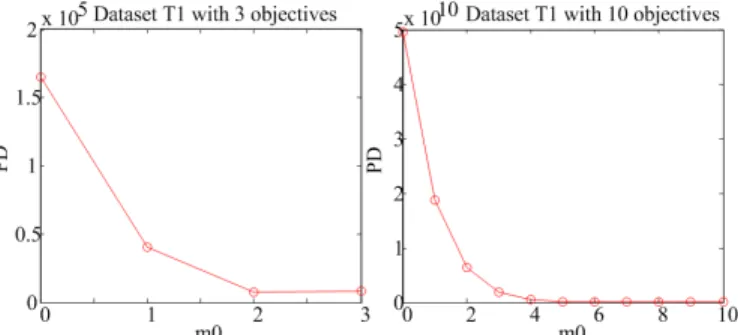
• Construct datasets T1(n, m, m0) with m0 objectives
fromU(n, m)and other objectives randomly sampled for 30 independent times, wherem0 increases from 1 to m.
Calculate their PD values.
• Construct datasets T2(n, m, K) with K randomly sam-pled fromU(n, m)and n−K randomly-sampled from
R(n, m) for 30 independent times, where K increases with a step of 10 solutions. Calculate their PD values. Fig. 11 shows the average PD values of dataset
T1(n, m, m0)with 3 and 10 objectives. When m0 increases,
the diversity of T1 decreases, because there are more ob-jectives having repeated values. As expected, the PD values decrease as m0 increases. Fig. 12 shows the average PD
values of datasetT2(n, m, K)with 3 and 10 objectives. AsK
Fig. 11. Average PD values of dataset T1(n, m, m0) with 3 and 10
objectives.
Fig. 12. Average PD values of datasetT2(n, m, K)with 3 and 10 objectives.
values, which decrease the diversity. Therefore, the PD value drops as K grows.
Solution sets with different degrees of convergence might have an impact on PD, because they might have different spreads. Taking a sampling set R from a true PF as an ex-ample, setsY1(g) =R+gandY2(g) =Rgare dominated by
R as shown in Fig. 13.Y1is shifted fromR, the dissimilarity
between solutions is not changed from R. Therefore, the PD value of Y1 equals to that of R. However, the scale of
Y2 is changed from R, Y2 has a larger spread than R, the
dissimilarity between solutions isg times as much asR, thus, the PD value of Y2 isg times as much asR.
Fig. 13. Illustration of setsY1 andY2.
From the above example in Fig. 13, it is clear that PD is a sole metric that measures diversity only, which cannot show any information about convergence. Convergence and diversity are two important aspects to evaluate the obtained solution set of MOPs. Unlike the mixed metrics such as IGD, sole metrics such as GD and PD cannot compare solution sets for convergence and diversity at the same time. Sole
metrics play a role of analyzing the reason why a solution set has poor performance. For example,Y2 has an IGD value
worse than R, which is hard to know the reason only from the IGD value. With the values of GD and PD, we can know that Y2 distributes far from the true PF and has a
larger spread than the true PF. As mentioned in [78], metrics compress the solution set into a single value to capture a certain characteristic. Multiple metrics should be employed to analyze the experimental results. Therefore, a combination of sole metrics for convergence and diversity as well as mixed metrics should be adopted to objectively evaluate solution sets, for instance, the combinations (GD, IGD, PD) and (∆p, PD) are highly recommended.
IV. DIVERSITYASSESSMENT OFMOEASUSING
PROPOSEDMETRIC
Not much work has been reported on comparing the di-versity maintenance performance of existing MOEAs. In this section, we use the proposed metric, PD to analyze the diversity maintenance performance of four MOEAs for solving MaOPs.
A. Test Problems and MOEAs under Comparison
DTLZ [79] and WFG [80] are two widely used MaOP test suites. We study the diversity of MOEAs on those problems with 2-10 objectives. The simulation includes four MOEAs for solving MaOps, including Two Arch2 [52], NSGA-III [50], IBEA (with Iε+) [21], and MOEA/D (T = 50)[18].
These MOEAs represent four different approaches in solving MaOPs. Two Arch2 is a hybrid method combining Pareto dominance and performance indicators; NSGA-III is a Pareto dominance based method with an additional mechanism for maintaining diversity with respect to a reference set; IBEA is a performance indicator based algorithm, and MOEA/D is a decomposition approach. To conduct a fair comparison, we use the same crossover (SBX with η = 15) and mutation (polynomial mutation withη= 15) for the compared MOEAs. 30 independent runs are performed for each MOEA with a maximum of 90000 function evaluations.
B. Performance of MOEAs in terms of PD
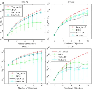
Each MOEA obtains a total of 100 solutions for compar-ison on the DTLZ and WFG problems. The PD values of Two Arch2, NSGA-III, IBEA, and MOEA/D on the problems with 2-10 objectives are shown in Figs. 14 and 15.
In Figs. 14 and 15, IBEA (with Iε+) has the worst PD
values on all low-dimensional problems. IBEA exhibits a clear advantage on convergence over others in solving MaOPs [12]. However, the diversity of the solution set obtained by IBEA is poor, because there is hardly any explicit diversity maintenance mechanism in IBEA. As shown in Fig. 16, IBEA performs the worst in terms of diversity on two multi-modal MaOPs, DTLZ1 and DTLZ3, as the solutions it has achieved cannot spread over the whole PF. For other MaOPs, the solutions achieved by IBEA spread randomly on the whole PF and the resulting PD values keep increasing as the number of objectives increases, as shown in Fig. 7.
Fig. 14. PD values of Two Arch2, NSGA-III, IBEA, and MOEA/D on the DTLZ problems with 2-10 objectives.
MOEA/D and NSGA-III perform differently from IBEA, as illustrated in Figs. 14, 15, and 16. On the multi-modal test functions, DTLZ1 and DTLZ3, the PD values of the solution sets obtained by MOEA/D and NSGA-III are better than that of the solutions achieved by IBEA because their solutions have better spread than those of IBEA. On the other MaOPs, MOEA/D and NSGA-III perform worse in terms of PD values than IBEA, which can be attributed to the fact that their solutions contain many repeated objective values, which is clearly observed in Fig. 16. Note that both MOEA/D and NSGA-III rely on a similar diversity maintenance mechanism. The former is based on a pre-defined set of weight vectors, whereas the latter is based on reference points. As a result, the diversity performance of both algorithms heavily depends on the pre-defined reference set. Very typically, these reference sets contain a large number of solutions having repeated values on each objective, which degrades the diversity in terms of PD values.
By contrast, Two Arch2 performs relatively poorly in terms of the PD values on 2- or 3-objective MOPs but performs the best in terms of the PD values on MaOPs having more than three objectives, as shown in Figs. 14 and 15. This is due to the fact that Two Arch2 adopts a different mechanism for diversi-ty maintenance from MOEA/D and NSGA-III. TheL p-norm-based diversity maintenance mechanism without any reference set that Two Arch2 employs can avoid the disadvantages of the reference set based diversity maintenance mechanism both MOEA/D and NSGA-III use. Note however that Two Arch2 is not best suited for solving MOPs with 2-3 objectives.
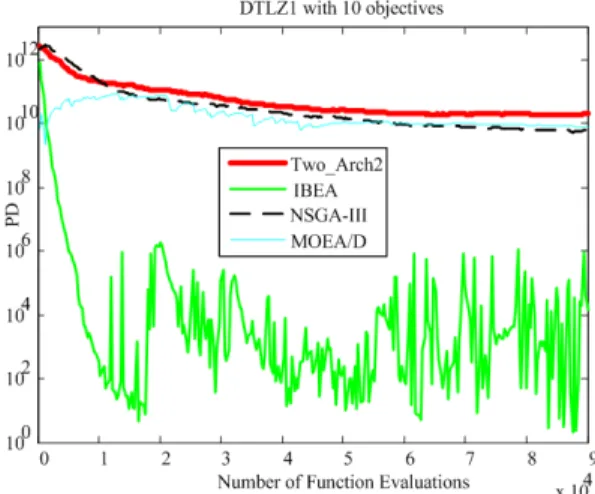
To show the diversity changes during the search of MOEAs in solving MaOPs, Fig.17 plots the average PD values over the generations of Two Arch2, NSGA-III, IBEA, and MOEA/D on DTLZ1 with 10 objectives. At the very beginning, the four
Fig. 15. PD values of Two Arch2, NSGA-III, IBEA, and MOEA/D on the WFG problems with 2-10 objectives.
Fig. 16. Parallel coordinates of the solution set with the best PD values by Two Arch2, NSGA-III, IBEA, and MOEA/D on DTLZ1 with 10 objectives.
Fig. 17. Average PD values over generations of Two Arch2, NSGA-III, IBEA, and MOEA/D on DTLZ1 with 10 objectives.
algorithms all have a large PD value, because the solutions they obtain are distributed randomly in the high-dimensional space, resulting in good diversity in terms of PD. In the late generations, the population converge towards the true PF, reducing the PD values. It is noticed that IBEA performs the worst in terms of the PD value during the whole evolutionary research, while Two Arch2 obtains the best PD value. NSGA-III and MOEA/D show similar PD values that are better than those of IBEA but worse than Two Arch2.
V. PD-BASEDDIVERSITYMAINTENANCE AND
REFERENCESETGENERATION
The above empirical results suggest that PD is an effective and subject diversity metric independent of a reference set. In this section, we test the idea of using PD for diversity maintenance in selection, wherensolutions need to be selected from a population (Pc) having N candidate solutions. The PD-based selection in essence chooses the solution having the maximal degree of dissimilarity to the selected population in each iteration. The details of the PD-based diversity mainte-nance scheme are given in Algorithm 2.
Algorithm 2Pseudo code of the PD-based diversity mainte-nance scheme.
Input: Pc-population ofNcandidates,D-dissimilarity matrix of Pc,n-required size.
1: Set the index set of Pc asIc= [1 :N].
2: Set P andIs empty.
3: Move the first candidate fromPc toP and index 1 from
Ic toIs.
4: fork= 1 :n−1do
5: A = D(Ic, Is) // dissimilarity from candidates to selected solutions.
6: Find the nearest solution in Pc to each candidate inP according toA in each row.
7: d=min(A,[],2).
8: Find candidatei with the maximaldi.
9: Move thei-th solution from Pc toP and indexifrom
Ic toIs.
10: end for Output: P.
A. Simulation for PD-Based Diversity Maintenance Scheme In this subsection, we simulate the situation that MOEAs may encounter in maintaining diversity. We assume the PF is defined by ∑mi=1fi = 1, set P with n randomly generated solutions on the PF is considered to be the parent set, and setQ with3n random samplings is viewed as the variations ofP. We employ the PD-based diversity maintenance scheme on P ∪Q to selectn solutions Pn as the parent set for the next generation for 30 times. We compare the PD values of P and Pn in Table II, where the results are analyzed using Wilcoxon signed-rank tests [81]. In the population with 100 solutions, the PD-based diversity maintenance mechanism significantly improves the diversity of the population for the next generation except for the 2-objective case, because of the small number of objectives and the small population size n. When the population sizenincreases to 200, the improvement becomes greater than the case of n = 100. To conclude, the PD-based diversity maintenance scheme is effective for MOEAs in solving MaOPs.
B. Simulation for PD-Based Reference Set Generation As the results in Section IV-B show, the diversity perfor-mance of the reference-based MOEAs in solving MaOPs is limited in terms of PD values. Consequently, if the reference set used in these algorithms is generated based on PD, their performance on diversity can be improved. The reference points can be selected by maximizing the PD value from a much larger initial set that is generated either randomly or using an existing method such as the one proposed in [18].
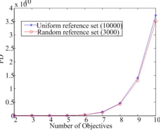
In this experiment, 100 solutions are selected from a random reference set with 3000 points and a uniform reference set with 10000 points, respectively. Fig. 18 shows the PD values of reference sets with 2-10 objectives using the PD-based reference set generation scheme. We find that a uniformly selected reference set containing 10000 points can achieve the same diversity level of a randomly generated reference
TABLE II
PDVALUES OFP(PARENT POPULATION)ANDPn(SELECTED POPULATION BY THEPD-BASED DIVERSITY MAINTENANCE SCHEME). RESULTS ARE ANALYZED USINGWILCOXON SIGNED-RANK TEST.
n= 100 n= 200
Obj # P Pn P Pn
2 1.6162e+03±2.1099e+02 1.7339e+03±2.3570e+02 1.8129e+03±2.4503e+02 1.9489e+03±2.1205e+02
3 1.5928e+05±1.0169e+04 2.2184e+05±5.6274e+03 2.1922e+05±9.8770e+03 3.0502e+05±3.8101e+03
4 3.2375e+06±1.5822e+05 4.6241e+06±1.0429e+05 5.0011e+06±1.5294e+05 7.1498e+06±1.1297e+05
5 3.0798e+07±9.1594e+05 4.3179e+07±9.3915e+05 4.9674e+07±1.4424e+06 6.9709e+07±7.3509e+05
6 1.8432e+08±4.8132e+06 2.5407e+08±3.2081e+06 3.1189e+08±6.3874e+06 4.2528e+08±4.1760e+06
7 8.2660e+08±2.4181e+07 1.1120e+09±1.4090e+07 1.4230e+09±3.1177e+07 1.9016e+09±1.6540e+07
8 3.0117e+09±8.1670e+07 3.9801e+09±4.7710e+07 5.2839e+09±1.0238e+08 6.9010e+09±5.3581e+07
9 9.4154e+09±1.9182e+08 1.2056e+10±1.5229e+08 1.6523e+10±2.3478e+08 2.1191e+10±2.0042e+08
10 2.5594e+10±4.2749e+08 3.2446e+10±3.0182e+08 4.5737e+10±7.0830e+08 5.7618e+10±4.0182e+08
set containing 3000 points. Fig. 19 presents the reference set after the PD-based selection for 3-objective problems. Both sets have good diversity. Thus, a reference set selected based on the PD value can enable reference-based MOEAs to achieve solutions of better diversity.
Fig. 18. PD values of reference sets with 2-10 objectives after the selection by PD guidance.
Fig. 19. Reference sets with 3 objectives after the selection by PD guidance from a random reference set with 3000 points and a uniform reference set with 10000 points.
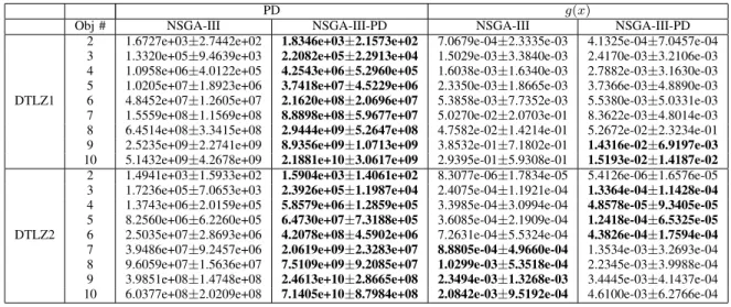
We replace the reference set generation method in NSGA-III with the PD-based method, which is termed NSGA-NSGA-III-PD for convenience. We compare NSGA-III and NSGA-III-PD on DTLZ1 and DTLZ2 with 2-10 objectives. We use g(x) that is a part of the DTLZ problems to show the performance of convergence as [39] and PD to assess diversity. The results are shown in Table III, which are analyzed using the Wilcoxon signed-rank test [81]. It is clear that the new reference set generated using the PD-based scheme significantly improves the diversity performance of NSGA-III on all the test prob-lems. Furthermore, the PD-based reference set generation has
no negative effect on the convergence of DTLZ1 with 2-8 objectives, but improves the convergence of DTLZ1 with more than 8 objectives and DTLZ2 with 2-6 objectives. Note that the PD-based reference set generation degrades the convergence performance of NSGA-III on DTLZ2 with more than 6 objec-tives, which remains unclear. Nevertheless, we can conclude that the PD-based reference set generation scheme can improve the diversity of reference-based MOEAs for MaOPs.
VI. CONCLUSIONS
A bio-inspired diversity metric, termed pure diversity (PD), is proposed to assess the performance of diversity of MOEAs for solving MaOPs. PD is a sum of the dissimilarity of solutions to the rest of the population in a greedy order, and the solution with the maximal dissimilarity has the highest priority to accumulate its dissimilarity. Thus, the diversity can be presented by the main dissimilarity in the population.
Through experiments on synthetic datasets, we show that PD is able to properly indicate the diversity of the population. Consequently, we used PD to assess the diversity of four MOEAs for solving MaOPs and analyze the characteristics of their diversity maintenance mechanisms. From the experi-mental results, we find that IBEA cannot achieve an adequately diverse solution set for MaOPs. Neither MOEA/D nor NSGA-III is able to maintain a large degree of diversity because their solution sets contain many solutions whose objective values heavily overlap. Independent of a reference set, theL p-norm-based diversity maintenance in Two Arch2 outperforms MOEA/D and NSGA-III in terms of PD values.
A PD-based diversity maintenance is also proposed for MOEAs, which is shown to be able to significantly improve solution diversity. Further, the PD-based diversity maintenance can be employed for the reference set generation in reference-based MOEAs, such as NSGA-III and MOEA/D, if the refer-ence set is selected from a much larger referrefer-ence set using the PD-based diversity maintenance scheme. It is shown that the diversity of NSGA-III is improved after embedding the new PD-based reference set generation method.
Although it can assess the diversity of the population of MOEAs for solving MaOPs, PD cannot be solely used to compare two solution sets for both convergence and diversity. A combination of different metrics should be adopted to completely evaluate the performance of MOEAs.
Much work remains to be done in the future. First, the com-plex relationship between convergence and diversity in
many-TABLE III
PDANDg(x)VALUES OFNSGA-IIIANDNSGA-III-PDONDTLZ1ANDDTLZ2WITH2-10OBJECTIVES. RESULTS ARE ANALYZED BY THE
WILCOXON SIGNED-RANK TEST.
PD g(x)
Obj # NSGA-III NSGA-III-PD NSGA-III NSGA-III-PD
DTLZ1
2 1.6727e+03±2.7442e+02 1.8346e+03±2.1573e+02 7.0679e-04±2.3335e-03 4.1325e-04±7.0457e-04 3 1.3320e+05±9.4639e+03 2.2082e+05±2.2913e+04 1.5029e-03±3.3840e-03 2.4170e-03±3.2106e-03 4 1.0958e+06±4.0122e+05 4.2543e+06±5.2960e+05 1.6038e-03±1.6340e-03 2.7882e-03±3.1630e-03 5 1.0205e+07±1.8923e+06 3.7418e+07±4.5229e+06 2.3350e-03±1.8665e-03 3.7366e-03±4.8890e-03 6 4.8452e+07±1.2605e+07 2.1620e+08±2.0696e+07 5.3858e-03±7.7352e-03 5.5380e-03±5.0331e-03 7 1.5559e+08±1.1569e+08 8.8898e+08±5.9677e+07 5.0270e-02±2.0703e-01 8.3622e-03±4.8014e-03 8 6.4514e+08±3.3415e+08 2.9444e+09±5.2647e+08 4.7582e-02±1.4214e-01 5.2672e-02±2.3234e-01 9 2.5235e+09±2.2741e+09 8.9356e+09±1.0713e+09 3.8532e-01±7.1802e-01 1.4316e-02±6.9197e-03
10 5.1432e+09±4.2678e+09 2.1881e+10±3.0617e+09 2.9395e-01±5.9308e-01 1.5193e-02±1.4187e-02
DTLZ2
2 1.4941e+03±1.5933e+02 1.5904e+03±1.4061e+02 8.3077e-06±1.7834e-05 5.4126e-06±1.6576e-05 3 1.7236e+05±7.0653e+03 2.3926e+05±1.1987e+04 2.4075e-04±1.1921e-04 1.3364e-04±1.1428e-04
4 1.3743e+06±2.0159e+05 5.8579e+06±1.2859e+05 3.3985e-04±3.0994e-04 4.8578e-05±9.3405e-05
5 8.2560e+06±6.2260e+05 6.4730e+07±7.3188e+05 3.6085e-04±2.1909e-04 1.2418e-04±6.5325e-05
6 2.5035e+07±2.8693e+06 4.2078e+08±4.5902e+06 7.2631e-04±5.5324e-04 4.3826e-04±1.7594e-04
7 3.9486e+07±9.2457e+06 2.0619e+09±2.3283e+07 8.8805e-04±4.9660e-04 1.3534e-03±3.2693e-04 8 9.6059e+07±1.5636e+07 7.5109e+09±9.2085e+07 1.0299e-03±5.3518e-04 2.2345e-03±3.9988e-04 9 3.9851e+08±1.4748e+08 2.4613e+10±2.8665e+08 2.3494e-03±1.3268e-03 3.4445e-03±4.1437e-04 10 6.0377e+08±2.0209e+08 7.1405e+10±8.7984e+08 2.0842e-03±9.5192e-04 4.6100e-03±6.2766e-04
objective optimization needs better understanding. Second, more experiments need to be done to verify the effectiveness of PD on MaOPs having complex PFs. Finally, the impact of
p in Lp-norm based distance on the dissimilarity of MaOPs needs further investigation.
REFERENCES
[1] V. Khare, X. Yao, and K. Deb, “Performance scaling of multi-objective evolutionary algorithms,” inEvolutionary Multi-Criterion Optimization, ser. Lecture Notes in Computer Science, C. Fonseca, P. Fleming, E. Zitzler, L. Thiele, and K. Deb, Eds. Springer Berlin / Heidelberg, 2003, vol. 2632, pp. 376–390.
[2] K. Deb, Multi-objective optimization using evolutionary algorithms. Wiley, 2001, vol. 16.
[3] P. Fleming, R. Purshouse, and R. Lygoe, “Many-objective optimization: An engineering design perspective,” in Evolutionary Multi-Criterion Optimization. Springer, 2005, pp. 14–32.
[4] J. O. Jansen, J. J. Morrison, H. Wang, R. Lawrenson, G. Egan, S. He, and M. K. Campbell, “Optimizing trauma system design: The GEOS (geospatial evaluation of systems of trauma care) approach,”Journal of Trauma and Acute Care Surgery, vol. 76, no. 4, pp. 1035–1040, 2014. [5] Y. Lei, M. Gong, J. Zhang, W. Li, and L. Jiao, “Resource allocation model and double-sphere crowding distance for evolutionary multi-objective optimization,”European Journal of Operational Research, vol. 234, no. 1, pp. 197–208, 2014.
[6] Y. Chi and J. Liu, “Learning of fuzzy cognitive maps with varying densities using a multiobjective evolutionary algorithm,”Fuzzy Systems, IEEE Transactions on, vol. 24, no. 1, pp. 71–81, 2016.
[7] K. Praditwong and X. Yao, “How well do multi-objective evolutionary algorithms scale to large problems,” inEvolutionary Computation, 2007. CEC 2007. IEEE Congress on. IEEE Press, 2007, pp. 3959–3966. [8] K. Miettinen,Nonlinear multiobjective optimization. Springer, 1999. [9] T. Wagner, N. Beume, and B. Naujoks, “Pareto-, aggregation-, and
indicator-based methods in many-objective optimization,” in Evolution-ary Multi-Criterion Optimization. Springer, 2007, pp. 742–756. [10] B. Li, J. Li, K. Tang, and X. Yao, “Many-objective evolutionary
algorithms: A survey,”ACM Computing Surveys (CSUR), vol. 48, no. 1, p. 13, 2015.
[11] H. Ishibuchi, N. Tsukamoto, and Y. Nojima, “Evolutionary many-objective optimization: A short review,” inEvolutionary Computation, 2008. CEC 2008. IEEE Congress on. IEEE Press, 2008, pp. 2419–2426. [12] D. Hadka and P. Reed, “Diagnostic assessment of search controls and failure modes in many-objective evolutionary optimization,” Evolution-ary Computation, vol. 20, no. 3, pp. 423–452, 2012.
[13] M. Gong, L. Jiao, H. Du, and L. Bo, “Multiobjective immune algorithm with nondominated neighbor-based selection,”Evolutionary Computa-tion, vol. 16, no. 2, pp. 225–255, 2008.
[14] K. Deb and S. Tiwari, “Omni-optimizer: A procedure for single and multi-objective optimization,” inEvolutionary Multi-Criterion Optimiza-tion. Springer, 2005, pp. 47–61.
[15] K. McClymont and E. Keedwell, “Deductive sort and climbing sort: New methods for non-dominated sorting,”Evolutionary Computation, vol. 20, no. 1, pp. 1–26, 2012.
[16] H. Wang and X. Yao, “Corner sort for Pareto-based many-objective optimization,”Cybernetics, IEEE Transactions on, vol. 44, no. 1, pp. 92–102, 2014.
[17] X. Zhang, Y. Tian, R. Cheng, and Y. Jin, “An efficient approach to nondominated sorting for evolutionary multiobjective optimization,” Evolutionary Computation, IEEE Transactions on, vol. 19, no. 2, pp. 201–213, 2015.
[18] Q. Zhang and H. Li, “MOEA/D: A multiobjective evolutionary algorithm based on decomposition,”Evolutionary Computation, IEEE Transactions on, vol. 11, no. 6, pp. 712–731, 2007.
[19] H. Ishibuchi, Y. Hitotsuyanagi, H. Ohyanagi, and Y. Nojima, “Effects of the existence of highly correlated objectives on the behavior of MOEA/D,” in Evolutionary Multi-Criterion Optimization. Springer, 2011, pp. 166–181.
[20] I. Giagkiozis, R. C. Purshouse, and P. J. Fleming, “Generalized decom-position and cross entropy methods for many-objective optimization,” Research Report No. 1029, Department of Automatic Control and Systems Engineering, 2012.
[21] E. Zitzler and S. K¨unzli, “Indicator-based selection in multiobjective search,” inParallel Problem Solving from Nature-PPSN VIII. Springer, 2004, pp. 832–842.
[22] E. Zitzler and L. Thiele, “Multiobjective evolutionary algorithms: A comparative case study and the strength Pareto approach,”Evolutionary Computation, IEEE Transactions on, vol. 3, no. 4, pp. 257–271, 1999. [23] J. Bader and E. Zitzler, “HypE: An algorithm for fast hypervolume-based many-objective optimization,”Evolutionary Computation, vol. 19, no. 1, pp. 45–76, 2011.
[24] ——, “A hypervolume-based optimizer for high-dimensional objective spaces,” inNew Developments in Multiple Objective and Goal Program-ming. Springer, 2010, pp. 35–54.
[25] N. Beume, B. Naujoks, and M. Emmerich, “SMS-EMOA: Multiobjec-tive selection based on dominated hypervolume,”European Journal of Operational Research, vol. 181, no. 3, pp. 1653–1669, 2007. [26] L. While, L. Bradstreet, and L. Barone, “A fast way of calculating
exact hypervolumes,”Evolutionary Computation, IEEE Transactions on, vol. 16, no. 1, pp. 86–95, 2012.
[27] K. Bringmann, “Bringing order to special cases of Klee’s measure problem,” in Mathematical Foundations of Computer Science 2013. Springer, 2013, pp. 207–218.
[28] L. Bradstreet, L. While, and L. Barone, “A fast many-objective hypervol-ume algorithm using iterated incremental calculations,” inEvolutionary Computation, 2010. CEC 2010. IEEE Congress on. IEEE, 2010, pp. 1–8.
R2 indicator,” inProceeding of the 14th annual conference on Genetic and evolutionary computation conference (GECCO). ACM, 2012, pp. 465–472.
[30] A. Diaz-Manriquez, G. Toscano-Pulido, C. Coello, R. Landa-Becerra et al., “A ranking method based on the R2 indicator for many-objective optimization,” in Evolutionary Computation, 2013. CEC 2013. IEEE Congress on. IEEE, 2013, pp. 1523–1530.
[31] R. Hernandez Gomez and C. Coello Coello, “MOMBI: A new meta-heuristic for many-objective optimization based on the R2 indicator,” in Evolutionary Computation, 2013. CEC 2013. IEEE Congress on. IEEE, 2013, pp. 2488–2495.
[32] D. Brockhoff and E. Zitzler, “Objective reduction in evolutionary mul-tiobjective optimization: theory and applications,”Evolutionary Compu-tation, vol. 17, no. 2, pp. 135–166, 2009.
[33] H. Wang and X. Yao, “Objective reduction based on nonlinear cor-relation information entropy,” Soft Computing, pp. 1–15, 2015, dOI: 10.1007/s00500-015-1648-y.
[34] D. Cvetkovic and I. C. Parmee, “Preferences and their application in evolutionary multiobjective optimization,” Evolutionary Computation, IEEE Transactions on, vol. 6, no. 1, pp. 42–57, 2002.
[35] D. Brockhoff and E. Zitzler, “Are all objectives necessary? on di-mensionality reduction in evolutionary multiobjective optimization,” in Parallel Problem Solving from Nature-PPSN IX. Springer, 2006, pp. 533–542.
[36] A. L´opez Jaimes, C. Coello Coello, and D. Chakraborty, “Objective reduction using a feature selection technique,” inProceeding of the 10th annual conference on Genetic and evolutionary computation conference (GECCO). ACM Press, 2008, pp. 673–680.
[37] K. Deb and D. Saxena, “On finding Pareto-optimal solutions through dimensionality reduction for certain large-dimensional multi-objective optimization problems,”Kangal report, vol. 2005011, 2005.
[38] D. Saxena and K. Deb, “Non-linear dimensionality reduction procedures for certain large-dimensional multi-objective optimization problems: Employing correntropy and a novel maximum variance unfolding,” in Evolutionary Multi-Criterion Optimization. Springer, 2007, pp. 772– 787.
[39] D. K. Saxena, J. A. Duro, A. Tiwari, K. Deb, and Q. Zhang, “Ob-jective reduction in many-ob“Ob-jective optimization: Linear and nonlinear algorithms,”Evolutionary Computation, IEEE Transactions on, vol. 17, no. 1, pp. 77–99, 2013.
[40] J.-H. Kim, J.-H. Han, Y.-H. Kim, S.-H. Choi, and E.-S. Kim, “Preference-based solution selection algorithm for evolutionary multi-objective optimization,”Evolutionary Computation, IEEE Transactions on, vol. 16, no. 1, pp. 20–34, 2012.
[41] R. Wang, R. Purshouse, and P. Fleming, “Preference-inspired coevo-lutionary algorithms for many-objective optimization,” Evolutionary Computation, IEEE Transactions on, vol. 17, no. 4, pp. 474–494, 2013. [42] K. Sindhya, A. B. Ruiz, and K. Miettinen, “A preference based inter-active evolutionary algorithm for multi-objective optimization: PIE,” in Evolutionary Multi-Criterion Optimization. Springer, 2011, pp. 212– 225.
[43] L. Thiele, K. Miettinen, P. Korhonen, and J. Molina, “A preference-based evolutionary algorithm for multi-objective optimization,”Evolutionary Computation, vol. 17, no. 3, pp. 411–436, 2009.
[44] K. Bringmann, T. Friedrich, F. Neumann, and M. Wagner, “Approximation-guided evolutionary multi-objective optimization,” inProceedings of the Twenty-Second international joint conference on Artificial Intelligence-Volume Two. AAAI Press, 2011, pp. 1198–1203. [45] M. Wagner and F. Neumann, “A fast approximation-guided evolutionary multi-objective algorithm,” inProceeding of the 15th annual conference on Genetic and evolutionary computation conference (GECCO). ACM Press, 2013, pp. 687–694.
[46] H. Sato, H. E. Aguirre, and K. Tanaka, “Controlling dominance area of solutions and its impact on the performance of MOEAs,” inEvolutionary Multi-Criterion Optimization. Springer, 2007, pp. 5–20.
[47] S. Kukkonen and J. Lampinen, “Ranking-dominance and many-objective optimization,” in Evolutionary Computation, 2007. CEC 2007. IEEE Congress on. IEEE Press, 2007, pp. 3983–3990.
[48] M. K¨oppen, R. Vicente-Garcia, and B. Nickolay, “Fuzzy-Pareto-dominance and its application in evolutionary multi-objective optimiza-tion,” inEvolutionary Multi-Criterion Optimization. Springer, 2005, pp. 399–412.
[49] M. Li, S. Yang, and X. Liu, “Pareto or non-Pareto: Bi-criterion evolution in multi-objective optimization,” Evolutionary Computa-tion, IEEE Transactions on, vol. PP, no. 99, pp. 1–21, 2015, dOI: 10.1109/TEVC.2015.2504730.
[50] K. Deb and H. Jain, “An evolutionary many-objective optimization algo-rithm using reference-point-based nondominated sorting approach, part I: Solving problems with box constraints,”Evolutionary Computation, IEEE Transactions on, vol. 18, no. 4, pp. 577–601, 2014.
[51] X. Zhang, Y. Tian, and Y. Jin, “A knee point-driven evolutionary algorithm for many-objective optimization,”Evolutionary Computation, IEEE Transactions on, vol. 19, no. 6, pp. 761–776, 2015.
[52] H. Wang, L. Jiao, and X. Yao, “Two Arch2: An improved two-archive algorithm for many-objective optimization,”Evolutionary Computation, IEEE Transactions on, vol. 19, no. 4, pp. 524–541, 2015.
[53] K. Li, S. Kwong, and K. Deb, “A dual-population paradigm for evo-lutionary multiobjective optimization,” Information Sciences, vol. 309, pp. 50–72, 2015.
[54] G. Yen and Z. He, “Performance metric ensemble for multiobjective evolutionary algorithms,”Evolutionary Computation, IEEE Transactions on, vol. 18, no. 1, pp. 131–144, 2014.
[55] M. Li, S. Yang, and X. Liu, “Diversity comparison of Pareto front approximations in many-objective optimization,” Cybernetics, IEEE Transactions on, vol. PP, no. 99, pp. 1–17, 2014, dOI: 10.1109/TCY-B.2014.2310651.
[56] D. A. Van Veldhuizen, “Multiobjective evolutionary algorithms: classi-fications, analyses, and new innovations,” DTIC Document, Tech. Rep., 1999.
[57] K. C. Tan, T. H. Lee, and E. F. Khor, “Evolutionary algorithms for multi-objective optimization: performance assessments and comparison-s,”Artificial Intelligence Review, vol. 17, no. 4, pp. 251–290, 2002. [58] E. Zitzler, K. Deb, and L. Thiele, “Comparison of multiobjective
evolutionary algorithms: Empirical results,”Evolutionary Computation, vol. 8, no. 2, pp. 173–195, 2000.
[59] S. Bandyopadhyay, S. Pal, and B. Aruna, “Multiobjective GAs, quantita-tive indices, and pattern classification,”Cybernetics, IEEE Transactions on, vol. 34, no. 5, pp. 2088–2099, 2004.
[60] O. Schutze, X. Esquivel, A. Lara, and C. A. Coello Coello, “Using the averaged hausdorff distance as a performance measure in evolutionary multiobjective optimization,”Evolutionary Computation, IEEE Transac-tions on, vol. 16, no. 4, pp. 504–522, 2012.
[61] Q. Zhang, A. Zhou, S. Zhao, P. Suganthan, W. Liu, and S. Tiwari, “Multiobjective optimization test instances for the CEC 2009 spe-cial session and competition,” University of Essex, Colchester, UK and Nanyang Technological University, Singapore, Special Session on Performance Assessment of Multi-Objective Optimization Algorithms, Technical Report, pp. 1–30, 2008.
[62] G. Rudolph, O. Sch¨utze, C. Grimme, C. Dom´ınguez-Medina, and H. Trautmann, “Optimal averaged Hausdorff archives for bi-objective problems: theoretical and numerical results,”Computational Optimiza-tion and ApplicaOptimiza-tions, pp. 1–30, 2015.
[63] D. A. Van Veldhuizen and G. B. Lamont, “On measuring multiobjective evolutionary algorithm performance,” in Evolutionary Computation, 2000. CEC 2000. IEEE Congress on, vol. 1. IEEE, 2000, pp. 204–211. [64] J. Wu and S. Azarm, “Metrics for quality assessment of a multiobjective design optimization solution set,” Journal of Mechanical Design, vol. 123, no. 1, pp. 18–25, 2001.
[65] A. Farhang-Mehr and S. Azarm, “Diversity assessment of Pareto optimal solution sets: an entropy approach,” in Computational Intelligence, Proceedings of the World on Congress on, vol. 1. IEEE, 2002, pp. 723–728.
[66] S. Mostaghim and J. Teich, “A new approach on many objective diversity measurement,”In Practical Approaches to Multi-Objective Optimization, vol. 04461, pp. 1–15, 2005.
[67] K. Deb and S. Jain, “Running performance metrics for evolu-tionary multi-objective optimizations,” in Proceedings of the Fourth Asia-Pacific Conference on Simulated Evolution and Learning (SEAL’02),(Singapore). Proceedings of the Fourth Asia-Pacific Con-ference on Simulated Evolution and Learning (SEAL’02),(Singapore), 2002, pp. 13–20.
[68] Y.-N. Wang, L.-H. Wu, and X.-F. Yuan, “Multi-objective self-adaptive differential evolution with elitist archive and crowding entropy-based diversity measure,”Soft Computing, vol. 14, no. 3, pp. 193–209, 2010. [69] L. Parsons, E. Haque, and H. Liu, “Subspace clustering for high dimensional data: a review,” ACM SIGKDD Explorations Newsletter, vol. 6, no. 1, pp. 90–105, 2004.
[70] A. Auger, J. Bader, D. Brockhoff, and E. Zitzler, “Theory of the hypervolume indicator: optimal µ-distributions and the choice of the reference point,” in Proceedings of the tenth ACM SIGEVO workshop on Foundations of genetic algorithms. ACM, 2009, pp. 87–102. [71] G. Rudolph, H. Trautmann, S. Sengupta, and O. Sch¨utze, “Evenly
triangulation,” inEvolutionary Multi-Criterion Optimization. Springer, 2013, pp. 443–458.
[72] C. Dominguez-Medina, G. Rudolph, O. Schutze, and H. Trautmann, “Evenly spaced pareto fronts of quad-objective problems using PSA partitioning technique,” inEvolutionary Computation (CEC), 2013 IEEE Congress on. IEEE, 2013, pp. 3190–3197.
[73] C. A. Rodr´ıguez Villalobos and C. A. Coello Coello, “A new multi-objective evolutionary algorithm based on a performance assessment indicator,” inProceeding of the 14th annual conference on Genetic and evolutionary computation conference (GECCO). ACM, 2012, pp. 505– 512.
[74] A. Solow, S. Polasky, and J. Broadus, “On the measurement of biolog-ical diversity,”Journal of Environmental Economics and Management, vol. 24, no. 1, pp. 60–68, 1993.
[75] C. C. Aggarwal, A. Hinneburg, and D. A. Keim, On the surprising behavior of distance metrics in high dimensional space. Springer, 2001.
[76] R. Morgan and M. Gallagher, “Sampling techniques and distance metrics in high dimensional continuous landscape analysis: Limitations and im-provements,”Evolutionary Computation, IEEE Transactions on, vol. 18, no. 3, pp. 456–461, 2014.
[77] E. Carreno Jara, “Multi-objective optimization by using evolutionary algorithms: The p-optimality criteria,”Evolutionary Computation, IEEE Transactions on, vol. 18, no. 2, pp. 167–179, April 2014.
[78] H. Wang, L. Jiao, R. Shang, S. He, and F. Liu, “A memetic optimization strategy based on dimension reduction in decision space,”Evolutionary Computation, vol. 23, no. 1, pp. 69–100, 2015.
[79] K. Deb, L. Thiele, M. Laumanns, and E. Zitzler, “Scalable multi-objective optimization test problems,” in Evolutionary Computation, 2002. CEC 2002. IEEE Congress on. IEEE Press, 2002, pp. 825–830. [80] S. Huband, P. Hingston, L. Barone, and L. While, “A review of multiob-jective test problems and a scalable test problem toolkit,”Evolutionary Computation, IEEE Transactions on, vol. 10, no. 5, pp. 477–506, 2006. [81] M. Hollander and D. Wolfe,Nonparametric statistical methods.
Wiley-Interscience, 1999.
Handing Wang (S’10-M’16) received the B.Eng. and Ph.D. degrees from Xidian University, Xi’an, China, in 2010 and 2015, respectively.
She is currently a research follow with the De-partment of Computer Science, University of Surrey, Guildford, UK.
Dr. Wang is a member of IEEE Computa-tional Intelligence Society. Her research interest-s include nature-ininterest-spired computation, multiobjec-tive optimization, multiple criteria decision mak-ing, surrogate-assisted evolutionary optimization, and real-world problems.
Yaochu Jin(M’98-SM’02-F’16) received the B.Sc., M.Sc., and Ph.D. degrees from Zhejiang University, Hangzhou, China, in 1988, 1991, and 1996 respec-tively, and the Dr.-Ing. degree from Ruhr University Bochum, Germany, in 2001.
He is a Professor of Computational Intelligence, Department of Computer Science, University of Sur-rey, Guildford, U.K., where he heads the Nature Inspired Computing and Engineering Group. He is also a Finland Distinguished Professor funded by the Finnish Agency for Innovation (Tekes) and a Changjiang Distinguished Visiting Professor appointed by the Ministry of Education, China. His science-driven research interests lie in the inter-disciplinary areas that bridge the gap between computational intelligence, computational neuroscience, and computational systems biology. He is also particularly interested in nature-inspired, real-world driven problem-solving. He has (co)authored over 200 peer-reviewed journal and conference papers and been granted eight patents on evolutionary optimization. His current research is funded by EC FP7, UK EPSRC and industry. He has delivered over 20 invited keynote speeches at international conferences.
He is the Editor-in-Chief of the IEEE TRANSACTIONS ON COGNITIVE AND DEVELOPMENTAL SYSTEMS and Complex & Intelligent Systems. He is also an Associate Editor or Editorial Board Member of the IEEE TRANSACTIONS ON EVOLUTIONARY COMPUTATION, IEEE TRANS-ACTIONS ON CYBERNETICS, IEEE TRANSTRANS-ACTIONS ON NANOBIO-SCIENCE, Evolutionary Computation, BioSystems, Soft Computing, and Natural Computing.
Dr Jin was an IEEE Distinguished Lecturer (2013-2015) and Vice President for Technical Activities of the IEEE Computational Intelligence Society (2014-2015). He was the recipient of the Best Paper Award of the 2010 IEEE Symposium on Computational Intelligence in Bioinformatics and Com-putational Biology and the 2014 IEEE ComCom-putational Intelligence Magazine Outstanding Paper Award. He is a Fellow of IEEE.
Xin Yao(M’91-SM’96-F’03) received the B.Sc. de-gree from the University of Science and Technology of China (USTC), Hefei, China, in 1982; the M.Sc. degree from North China Institute of Computing Technology, Beijing, China, in 1985; and the Ph.D. degree from the USTC, Hefei, in 1990.
He was an Associate Lecturer and Lecturer with the USTC, from 1985 to 1990; a Postdoctoral Fellow with the Australian National University, Canberra, Australia, and Commonwealth Scientific and Indus-trial Research Organization, Melbourne, Australia, from 1990 to 1992; and a Lecturer, Senior Lecturer, and Associate Professor with the University of New South Wales, the Australian Defence Force Academy (ADFA), Canberra, from 1992 to 1999. Since April 1999, he has been a Professor (Chair) of Computer Science with the University of Birmingham, U.K., where he is currently the Director of the Centre of Excellence for Research in Computational Intelligence and Applications.
Mr. Yao is an IEEE CIS Distinguished Lecturer and a former EIC of the IEEE TRANSACTIONS ON EVOLUTIONARY COMPUTATION. He was a recipient of the 2001 IEEE Donald G. Fink Prize Paper Award, the 2010 IEEE TRANSACTIONS ON EVOLUTIONARY COMPUTATION Outstanding Paper Award, the 2011 IEEE TRANSACTIONS ON NEURAL NETWORKS Outstanding Paper Award, and several other best paper awards.