Kent Academic Repository
Full text document (pdf)
Copyright & reuse
Content in the Kent Academic Repository is made available for research purposes. Unless otherwise stated all content is protected by copyright and in the absence of an open licence (eg Creative Commons), permissions for further reuse of content should be sought from the publisher, author or other copyright holder.
Versions of research
The version in the Kent Academic Repository may differ from the final published version.
Users are advised to check http://kar.kent.ac.uk for the status of the paper. Users should always cite the published version of record.
Enquiries
For any further enquiries regarding the licence status of this document, please contact: [email protected]
If you believe this document infringes copyright then please contact the KAR admin team with the take-down information provided at http://kar.kent.ac.uk/contact.html
Citation for published version
Oliveira, Luiz O.V.B. and Otero, Fernando E.B. and Miranda, Luis F. and Pappa, Gisele L. (2016)
Revisiting the Sequential Symbolic Regression Genetic Programming. In: Brazilian Conference
on Intelligent System (BRACIS 2016), 9-12 October 2016, Recife, Brazil. (In press)
DOI
Link to record in KAR
http://kar.kent.ac.uk/59290/
Document Version
Author's Accepted Manuscript
Revisiting the Sequential Symbolic Regression
Genetic Programming
Luiz Otavio V. B. Oliveira
∗, Fernando E. B. Otero
†, Luis F. Miranda
∗, Gisele L. Pappa
∗ ∗ Computer Science Department, Federal University of Minas Gerais, Belo Horizonte, Brazil{luizvbo,luisfmiranda,glpappa}@dcc.ufmg.br
† School of Computing, University of Kent, Chatham Maritime, UK [email protected]
Abstract—Sequential Symbolic Regression (SSR) is a technique that recursively induces functions over the error of the current solution, concatenating them in an attempt to reduce the error of the resulting model. As proof of concept, the method was previ-ously evaluated in one-dimensional problems and compared with canonical Genetic Programming (GP) and Geometric Semantic Genetic Programming (GSGP). In this paper we revisit SSR exploring the method behaviour in higher dimensional, larger and more heterogeneous datasets. We discuss the difficulties arising from the application of the method to more complex problems, e.g., overfitting, along with suggestions to overcome them. An experimental analysis was conducted comparing SSR to GP and GSGP, showing SSR solutions are smaller than those generated by the GSGP with similar performance and more accurate than those generated by the canonical GP.
I. INTRODUCTION
The divide and conquer strategy is a successful computa-tional paradigm that allows difficult problems to be solved by dividing them into smaller and more feasible problems. The area of machine learning employs this paradigm into a variety of algorithms, including decision trees [1] and rule learning [2]. These learning algorithms decompose a problem into subproblems, find solutions to these subproblems and use them to generate the solution for the original problem. A similar strategy is used by many rule induction algorithms, where a sequential covering strategy is used to transform the problem of finding a list of classification rules into a sequence of smaller problems of finding a single rule. After a rule is created, the training cases classified by the rule are removed from the training set, reducing the size of the dataset for the next iteration of the procedure.
Since the introduction of Genetic Programming (GP) [3], researchers have been interested in exploring the regularities and modularity of its search space [4]. One of the main motivations to identify these regularities is to decompose the problem at hand into more tractable subproblems, similarly to what the sequential covering and divide and conquer strategies do. One of the first attempts in GP to explore these regularities is the use of Automatic Defined Functions (ADFs) [3], [4]. ADFs provide a mechanism by which the evolutionary process can evolve reusable components—the ADFs—along with the main tree, and these components can be added to the tree as if they belong to the primitive set of functions used to initially generate the trees.
Other approach to deal with this problem was proposed by [5], which presented the Sequential Covering Genetic Pro-gramming (SCGP), a strategy based on the sequential covering to decompose a boolean problem into smaller subproblems. Each subproblem is then solved by a traditional GP and the individual solutions are combined using a geometric semantic crossover [6]. The geometric semantic crossover and mutation operators [6] are search operators that act on the syntax of the individuals producing an expected semantic outcome. The SCGP uses a property of the geometric semantic crossover for the boolean domain: individuals are combined using a boolean mask, which acts as a selector to inform when a particular individual solution should be used. While this strategy is successful for boolean domains, there is not a straightforward way to adapt it to the real domain, since the operation of the geometric semantic crossover is different.
The Sequential Symbolic Regression (SSR) [7] introduces a different strategy to employ the geometric semantic crossover in order to incrementally solve symbolic regression problems. The method starts with an empty solution that is iteratively constructed by combining new functions through a geometric semantic crossover operator. These functions are induced from the error relative to the difference between the solution found so far and the expected output. SSR employs a GP to search for function approximations and the geometric semantic crossover operator [6] to find the expected semantics of the complementary functions and combine them. The method was tested in eight polynomial functions, as a proof of concept, and presented a significant improvement in terms of the size of the solutions in relation to the original GSGP.
This paper extends SSR by investigating important aspects unanalysed in the original work. When applied to more complex datasets, SSR manifests overfitting and anomalous functioning. We discuss the origin of these undesired be-haviours and present simple solutions in order to reduce them. This paper also presents an experimental analysis in higher dimensional and larger datasets and the impact on the resulting solution of increasing the number of SSR iterations.
The remainder of this paper is organized as follows. Section II reviews previous works that combines regression models induced from the model’s error in an attempt to improve the final solution. Section III revisits the SSR method and proposes extensions to cope with problems arising from its application
to more complex datasets, including numeric overflow due to concatenation of expressions and overfitting. Section IV presents the experimental analysis in twenty different datasets followed by conclusions and research directions in Section V.
II. RELATEDWORK
The work presented in this paper is related to ensemble learning, in particular togradient boosting[8]. Ensembles are methods that generate several weak models that are combined to generate stronger classification or regression models [9]. The main principle behind gradient boosting is to learn new models with highest correlation to the negative gradient of the loss (error) function associated to the final ensemble output. Given a training set T ={(xi,yi)}
n
i=1 defined by an unknown function f∗(x), the method approximates f∗(x)by
f(x) =
M
∑
m=0
βmh(x;am) , (1)
where h(x;am) is the base (weak) learner—usually a simple
parameterized function characterized by a parameter vector am—and βm is the corresponding coefficient. The method
starts with an initial approximation, induced directly from T, and incrementally expands the model. The function h(x;am)
is fitted by adjusting the parameteramusing least-squares and
the optimal value of βm is determined by a line search.
When the loss function adopted is the quadratic error, the optimization process is similar to search by a model that approximates the residuals of the previous model found, similar to the idea presented in SSR.
However, even before the theoretical foundation given by gradient boosting, Lee [10] proposed a form of recursively adjust a symbolic regression function within the context of time series forecasting by Genetic Recursive Regression (GRR). GRR assumes real world time series are composed by a deterministic (fD) and a stochastic component (fS), such as
f=fD+fS . (2)
A traditional GP expresses the deterministic part while the time series’ residual, fS=f−fD, is again expanded into two
parts.
GRR assigns numerical coefficients to each function in-duced during the process and calculates them by the least squares method with respect to the training dataset. Panya-worayan and Wuetschner [11] presented a similar approach to GRR, also applied to time series forecasting. However, a genetic algorithm is used to adjust the values of the numerical coefficients instead of the least squares method.
A more recent method, named Multiple Regression GP (MRGP) [12], also assigns coefficients to the elements of the resulting function, which are optimized by regression. The method consists in a GP with selection strategy based on Non-dominated Sorting Genetic Algorithm II (NSGA-II) [13] with two minimization objectives, the model subtree complexity measure and the multiple regression error.
III. SEQUENTIALSYMBOLICREGRESSION
This section introduces Sequential Symbolic Regression (SSR), a method that sequentially builds a solution for sym-bolic regression problems by means of GP.
Given a training setT={(xi,yi)}
n
i=1—where(xi,yi)∈R
d×
R (i=1,2, ...,n) — a symbolic regression problem can be
defined as finding a function f :Rd→R that minimizes an
error metric in T.
The majority of the error metrics adopted for symbolic regression, such as the Mean Squared Error (MSE), the Mean Absolute Error (MAE), the Root Mean Squared Error (RMSE) or the coefficient of determination (R2) use the sum of the absolute or squared residuals—the difference between the current output and the function output—to compute their respective values. These metrics share a common property: the error quantified by the metric decreases when the absolute residuals are minimized. A residuale(f,T)corresponds to the
deviation of the fitted function f from the observed outputs in T. For each pair(xi,yi)inT, the residual is defined as
ei(f,T) =yi−yˆi=yi−f(xi) . (3)
The optimal solution to a regression problem is a function f∗ that perfectly fits the input data, i.e. where ei(f∗,T) =
yi−f∗(xi) =0 fori=1,2, ...,n. However, often the regression
model is just an approximation of f∗, not reaching a zero error or a predefined minimum error. Whenever the symbolic regression finds a suboptimal function f (i.e. ei(f,T)6=0 for
at least one observationi), the model can still be improved by adding a term that approximates the residuals.
SSR takes advantage of this property and employs the geometric semantic crossover operator [6] to subsequently combine suboptimal functions and approximations to their residuals. The main idea behind the geometric semantic crossover is to create a convex combination of two solutions to the problem being tackled. We use this operator to combine an initial approximation function f evolved overT with a new function fnew, generated over the residuals of f inT.
Alg. 1 presents the high-level pseudocode of the SSR proce-dure. The method starts with an empty solution treeS, which is incrementally constructed over the iterations and returned as the final regression model. At the beginning of iteration k, the desired outputs are normalized (line 6), as detailed in Section III-B. This procedure returns the normalized output set Ty′={y′i}ni=1and the mean and standard deviation calculated
during the process.
The original inputs and the normalized outputs define the training setT′={(xi,y′i)}
n
i=1, used by a standard GP to induce a function f (line 7). Following the GP execution, function isLastIterationchecks whether the maximum number of iter-ationsmaxIter is reached or if the function f corresponds to the optimal solution, i.e., has RMSE equals to zero. When any of the previous mentioned situations occur, f is added to the solution treeSand the sequential procedure stops, returningS. Otherwise, f is added to the solution treeSusing the geometric semantic crossover, and the outputs are updated to consider the
Algorithm 1: Sequential Symbolic Regression procedure Input:training points (T),maxIter, GP parameters
1 Tx←(x1,x2, ...,xn), forxi∈R
d ; // Inputs
2 Ty←(y1,y2, ...,yn), for yi∈R; // Outputs
3 S←/0 ; // Initially empty solution
4 k←1 ;
5 Loop
6 (Ty′,y¯,sy)←normalize(Ty); // Normalization 7 f←runGP(Tx,Ty′);
8 if isLastIteration( f,k) =TRUE then
9 if k=1 then // First scenario
10 S←y¯+sy·f;
11 else // Second scenario
12 fnew←y¯+sy·f; 13 return S
14 r←random();
15 if k=1 then // Third scenario
16 S←y¯+sy·[r·f+ (1−r)·fnew];
17 else // Fourth scenario
18 fnew←y¯+sy·[r·f+ (1−r)·fnew];
19 Ty←adjustOutputs(f,r,Ty′); 20 k←k+1;
residuals of the current solution (procedure adjustOutputs), which will be considered as the desired outputs in the next SSR (and consequently, next GP) iteration. The next sections detail all components of SSR.
A. Adding functions to the current solution
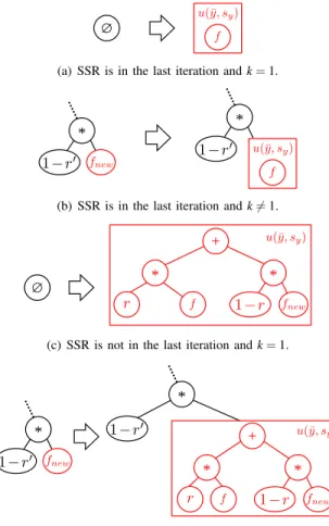
At each iteration k of SSR, the method adds the function found by GP—f—to the overall solution S. The way f is added to S varies depending whether the current iteration is or is not the first or the last iteration, generating four scenarios: SSR is in the last iteration and (1) k=1 or (2) k6=1, SSR is not in the last iteration and (3) k=1 or (4) k6=1. These scenarios are depicted in Figure 1.
Alg. 1 presents these four scenarios. The first scenario occurs when SSR finds the optimal solution in the first iteration or when maxIter =1. In this case (line 10), the method returns the equivalent to the output of a canonical GP with the normalization/denormalization stage presented in Section III-B. The second scenario takes place in the last iteration of the method—i.e., when the maximum number of iterations is reached or the optimal solution is found—when there was at least one other iteration (line 12). In this circumstance, the incomplete function generated in the previous iteration has its pointer fnewpointing to the generated function f, resulting in
a fully functional solution S, returned to the user.
The other two scenarios employ the geometric semantic crossover operator to append function f toS. The main idea behind this operator is to create a convex combination of two solutions, guaranteeing that the fitness of the new solution generated (in our case, RMSE) will never be worse than the worst of its parents. However, instead of applying the
∅
(a) SSR is in the last iteration andk=1.
* *
(b) SSR is in the last iteration andk6=1.
∅
+
* *
(c) SSR is not in the last iteration andk=1.
*
+ * *
*
(d) SSR is not in the last iteration andk6=1.
Fig. 1. AddFunctionscenarios. The boxu(y¯,sy)indicates the denormalization process regarding f, r′ represents the value of r defined in the previous iteration and nodes in red denote what is modified in the iteration. Scenarios (b) and (d) present only the rightmost subtree ofS(symbolized by a dashed line).
geometric semantic crossover to two parents, SSR applies it to one known parent—f—and to a pointer to be fulfilled with the second parent—fnew—in the next iteration, as presented
by:
r·f+ (1−r)·fnew , (4)
whereris random constant in[0,1).
Notice that the third and fourth scenarios occur only when the optimal solution is not found, i.e., when the procedure isLastIteration returns FALSE. Thus, the method can search in the next iteration by a function to be pointed by fnew, such
that the zero error is achieved. The difference between the third scenario (line 16) and the fourth (line 18) is that the former takes place in the first iteration, whenSis empty—Sis replaced by the output of the geometric semantic crossover— and the latter occurs in the subsequent iterations—Sis already defined and the current pointer fnewstarts to point to the output
of the geometric semantic crossover operator.
WhenSis modified by the third or fourth scenarios, SSR has to compute a new output set used to search for the function placed in fnew. The method adjustOutputs replaces f(xi) in
Eq. 3 by Eq. 4, equals the error ei(f,T) to zero and isolates
the pointer fnew in the left-hand side, leading to:
y(inew)=yi−r·f(xi)
1−r , (5)
where y(inew) is the output expected from the function placed in fnew andyi is in the output set used to find the function f
by the runGPprocedure.
B. Normalization and Denormalization Procedures
The normalization and denormalization processes are not present in the early SSR version [7]. They were introduced to avoid computations leading to anomalous behaviour, caused by approximations and double overflow. Let y(i0) be the i-th original desired output defined by the training set. We can generate any desired output for the k-th iteration of SSR as:
y(ik)= y(i0)−r1f1(xi)− k ∑ j=2 rjfj(xi) j−1 ∏ m=1 (1−rm) k ∏ j=1 (1−rj) , (6)
for k≥2. Let R={r1,r2, . . . ,rk} be equally distributed in
intervals defined in m
10,
m+1 10
for m=0,1, . . . ,9 (given the
random values of rm are uniformly distributed, this is a
viable proposition). We can calculate an upper bound for the denominator of (6) as k
∏
j=1 (1−rj)≤ 10∏
m=1 m 10 10k . (7)Whenkis sufficiently big this limit potentially leads to double overflow, e.g., fork=1000, this upper bound is approximately 9.47·10−
345. This is equivalent to multiplying the numerator by a number as big as 1.06·10
344. Even the single-precision 64-bit IEEE 754 floating point standard (used in Java and C++ double primitives) cannot handle such a big number, causing an overflow error. The normalization prevents this kind of problem by changing the function output range.
The new values of outputs are normalized as y′i=yi−y¯
sy
, (8)
where y′i is the normalized value, and ¯yand sy are the mean
and standard deviation ofTy, respectively.
In order to obtain values in the original range, the function f learned from the normalized data needs to be denormalized through ¯y+sy·f(xi)—see lines 10, 12, 16 and 18 in Alg. 1.
C. Mitigating Overfitting
Genetic Programming and other machine learning tech-niques are usually trained by maximizing their performance (fitness in evolutionary algorithm context) in some training data. However, the performance of a learned model is mea-sured in relation to unseen data and not to the training set. Overfitting occurs when the model performs well on the training data but very poorly on unseen instances.
We adopted two adjustments to reduce overfitting in SSR. The first is related to the use of protected operators in the GP function set. As presented by Keijzer [14], protected operators may induce asymptotes in regions of the input space not covered by the training set. When the GP induced function is applied to unseen data, it may generate arbitrarily high or low values inside these regions. In particular, when we iteratively induce functions over the residuals, as SSR does, the odds of this behaviour is even higher. The solution found to overcome this pitfall was to change the protected operators (only protected division in our case) by a similar operator with no discontinuity called analytic quotient (AQ), defined as
AQ(a,b) =
a √
1+b2 , (9)
given the positive results presented in [15].
The second adjustment is related to the training sample strategy adopted by the GP. Instead of using the entire training set T at each GP generation, we adopt our own variation of the Random Sample Technique (RST) [16] that randomly partitions the training set into k equal size disjoint subsets, T1,T2, . . . ,Tk, alternating among them at each s generations.
Only the last generation of the GP uses the whole training set T to select the best individual, which is the individual that will be added to the solution treeS.
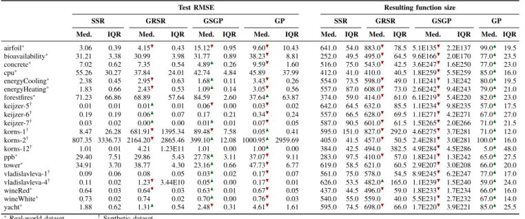
IV. EXPERIMENTALRESULTS
In this section we present an experimental analysis of SSR in a diversified collection of real-world and synthetic datasets. The results are compared with a canonical GP [3], the Geometric Semantic GP (GSGP) [17] and a modified version of GRR [10] for symbolic regression.
In contrast with the original GRR, developed for forecasting real world chaotic time series [10], the version adopted here was adapted for symbolic regression, and renamed Genetic Recursive Symbolic Regression (GRSR). GRSR does not use the parallel architecture with multiple populations or the derived terminal set from [10], and adopts the RMSE as fitness measure.
The main differences of the GRSR regarding SSR are: (i) the resulting solution combines the functions found by GP into a linear model; (ii) there is no need for normalization, once the function coefficients are adjusted by ordinary least squares; and (iii) its fitness function is based on the RMSE of S in relation to the original training set, while SSR uses the RMSE of the last generated function in relation to the normalized data.
The experimental test bed is composed of datasets selected from the UCI machine learning repository [18], GP bench-marks [19] and a previous work involving GSGP [20], as presented in the Table II. The categorical attributes from the Computer Hardware and the Forest Fires datasets were removed for compatibility purpose.
We defined different strategies for the experiments accord-ing to the nature and source of the datasets. For real datasets, we randomly partitioned the data into five disjoint sets of the
TABLE I
PARAMETERS USED BY EACH ALGORITHM DURING THE EXPERIMENTS.
Parameter SSR / GRSR GSGP GP Crossover probability 0.9 0.5 0.9 Mutation Probability 0.1 0.5 0.1 Tournament Size 7 10 7 Population Size 1000 1000 1000 Number of generations 200 2000 2000 Number of iterations 10 -
-same size and executed the methods ten times with a 5-fold cross-validations (10×5-CV). For the synthetic ones, we used two different strategies according to the way the dataset was defined in its original work: experiments with datasets keijzer-6 and keijzer-7 were deterministically sampled fifty times with the same data folds (50×D), while the other datasets were resampled five times and the experiments were repeated ten times for each sampling (10×5-ND). Training and test sets were sampled with the same strategy. The only exception was the Vladislavleva-1 dataset, where the training set was sampled following the 10×5-ND strategy and the test set was deterministic sampled once, following the original experiment [19]. At the end, all methods were executed 50 times.
In order to make a fair comparison with the baselines, we included the RST method presented in Section III-C in all methods, with s=10 and k=5. However, preliminary experiments showed that this strategy was prejudicial to GP and GSGP, and hence they do not adopt it. All methods use function set including three arithmetic operators (+,−,×) and
AQ as an alternative to the arithmetic division, and terminal set including the variables of the problem and constant values randomly picked from [−1,1]. The grow method [3] was
adopted to generate the random functions inside the geometric semantic crossover and mutation operators—within GSGP— and the ramped half-and-half method [3] was used to generate the initial population of all methods, both with maximum individual depth equals to six. Table I presents the parameters specific for each algorithm. All parameters were defined according to the results obtained in preliminary experiments. SSR, GRSR, GSGP and GP configurations respect a budget of 2 million evaluations. Note that the number of generations of SSR and GRSR is smaller because both run for 10 iterations. Table II presents the median and IQR (Interquartile Range) of the test RMSE and resulting function size, according to the 50 executions of each method. In order to analyse the statistical difference of the results, two comparisons were performed. First, pairwise comparisons among the methods were done using a t-test. The results are indicated by the symbols N(H), meaning the method in the cell is statistically better (worse) than SSR with 95% confidence. Then, we adopted the less conservative variant of the Friedman test proposed by Iman and Davenport [21], here called adjusted Friedman test. We performed one adjusted Friedman test under the null hypothesis that the performances of the methods— measured by their median test RMSE—are equal; and one under the null hypothesis that the median sizes of the resulting
expressions (functions) generated by the methods are equal. The p-valuesreported by both tests are presented in Table III, and implicate in discarding both null hypothesis with a confidence level of 95%. Thus, two Finner post-hoc tests [22] were performed to verify statistical differences among SSR and the other methods in relation to the RMSE and function size. The adjusted p-values(APV) resulting from these tests are presented in the last three columns from Table III. Again, the symbol N(H) indicates the method in the column is statistically better (worse) than SSR with 95% confidence.
The results show that there is no evidence of statistical difference in relation to the SSR and both GSGP and GRSR performances. Nevertheless, there is evidence that the SSR performs better than the GP. Analysing the function size, there is statistical evidence that the GP produces smaller function approximations than the SSR. Also the SSR solutions sizes are statistical smaller than those from the GSGP. Overall, SSR performs better than the GP in terms of test RMSE but generates bigger solutions; and there is no statistical evidence that the SSR and GSGP performance are different but there is strong evidence that SSR induced functions are smaller than those generated by the GSGP. These results indicate SSR is a better option than the canonical GP when the main goal is to obtain more accurate functions and the size of the solutions is not relevant. Furthermore, SSR is capable of producing solutions with similar accuracy to those produced by GSGP, but many orders of magnitude smaller, since the size of GSGP individuals grows exponentially in relation to the number of generations. Regarding the GRSR, there is no statistical evidence that its performance or resulting function size differ from those obtained by SSR.
V. CONCLUSIONS ANDFUTUREWORK
This paper revisited the Sequential Symbolic Regression and performed a deeper analysis over a more diversified test bed. We observed that SSR presented issues—including overfitting—when applied to more complex problems. In this paper we proposed extensions to mitigate these problems in order to improve the performance of the method.
Experiments were run in a test bed of twenty datasets, and results compared to a canonical GP, a Geometric Semantic GP (GSGP) and a to the Genetic Recursive Symbolic Regression (GRSR). When RMSE median was used as the performance metric, the results showed SSR performs statistically sig-nificantly better than the GP and presents no evidence of statistical difference to GSGP and GRSR. When comparing the size of the resulting functions, SSR solutions are statistically significantly smaller than those generated by the GSGP, but larger than those produced by the GP. These results indicate that SSR is a good alternative to GP when the performance is more important than the size of the functions; and to GSGP, where the RMSE obtained is similar but SSR generates smaller solutions, restraining the exponential grown caused by the indiscriminate use of semantic geometric operators by GSGP. Potential future developments involve investigating other methods of combing functions and to dynamically control
TABLE II
MEDIAN ANDIQROF THERMSEAND RESULTING FUNCTION SIZE FOR EACH ALGORITHM. THE SYMBOLN(H)INDICATES THE METHOD IN THE CELL IS STATISTICALLY BETTER(WORSE)THANSSRWITH95%CONFIDENCE,ACCORDING TO A T-TEST.
Test RMSE Resulting function size
SSR GRSR GSGP GP SSR GRSR GSGP GP Med. IQR Med. IQR Med. IQR Med. IQR Med. IQR Med. IQR Med. IQR Med. IQR
airfoil∗ 3.06 0.39 4.15H 0.43 15.12H 0.95 9.60H 10.43 641.0 54.0 883.0H 78.5 5.1E135H 2.2E137 99.0N 19.5 bioavailability∗ 31.21 3.38 30.99N 3.98 31.77N 0.89 38.23H 8.81 252.0 49.5 495.0H 64.5 9.6E166H 2.0E170 77.0N 23.5
concrete∗ 7.02 0.62 7.35N 0.54 4.89N 0.26 9.59H 1.60 516.0 75.0 543.0H 42.5 3.6E247H 1.6E250 77.0N 23.0
cpu∗ 55.26 30.27 37.84N 24.01 42.74N 4.84 45.89N 37.99 412.0 41.0 410.0N 40.5 1.8E259H 5.5E259 85.0N 16.0 energyCooling∗ 2.38 0.45 2.95H 0.63 1.68N 0.11 3.43H 0.26 554.0 73.5 598.0H 49.0 1.1E241H 1.3E242 80.0N 19.5 energyHeating∗ 1.83 0.66 2.43H 0.53 1.09N 0.14 3.05H 0.56 557.0 87.0 608.0H 73.0 2.6E242H 9.4E243 79.0N 21.0 forestfires∗ 71.23 66.86 68.89N 57.64 84.59N 2.60 37.64N 63.87 374.0 59.0 414.0H 61.0 6.1E219H 5.4E220 82.0N 23.0 keijzer-5† 0.01 0.01 0.01N 0.01 0.06H 0.00 0.03H 0.02 642.0 64.5 632.0N 85.5 1.1E234H 9.8E235 57.0N 17.5 keijzer-6† 0.19 0.19 0.06N 0.07 0.17N 0.21 0.34H 0.24 557.0 66.5 628.0H 69.5 1.1E271H 4.2E271 67.0N 27.0 keijzer-7† 0.03 0.02 0.00N 0.00 0.01N 0.01 0.07H 0.05 587.0 90.5 601.0H 61.5 1.5E265H 2.0E266 71.0N 21.5 korns-1† 8.47 26.28 681.91H 1395.34 89.48H 7.58 0.05N 0.41 595.0 151.0 827.0H 292.0 4.6E275H 3.7E281 71.0N 12.0 korns-2† 807.35 3336.73 2164.20H 2865.46 399.10N 12.08 1000.95N 2959.69 405.0 41.5 457.0H 50.5 2.4E281H 3.0E281 100.0N 16.0
korns-12† 1.01 0.01 4.21N 1.23E11 1.01N 0.00 1.00N 0.00 384.0 42.5 494.0N 382.5 4.9E284H 4.5E286 5.0N 48.0 ppb∗ 29.40 7.51 29.86N 5.43 27.78N 3.11 37.07H 9.11 283.0 97.5 410.0H 57.0 1.8E241H 1.3E242 65.0N 27.5 tower∗ 34.91 3.70 38.77N 4.30 23.16N 0.66 47.73H 6.77 619.0 58.5 621.0N 60.5 2.9E207H 3.0E208 66.0N 20.0 vladislavleva-1† 0.09 0.06 0.08N 0.05 0.03N 0.02 0.17H 0.07 561.0 75.0 578.0N 54.5 8.9E245H 6.2E247 77.0N 17.0 vladislavleva-4† 0.11 0.02 1.23H 3.44E10 0.05N 0.00 0.17H 0.01 626.0 53.5 482.0N 165.0 1.1E239H 1.5E240 59.0N 24.0 wineRed∗ 0.64 0.03 0.64H 0.03 0.63N 0.01 0.67H 0.05 437.0 44.5 496.0H 59.0 1.8E233H 1.7E234 66.0N 16.0 wineWhite∗ 0.73 0.02 0.74N 0.02 0.70N 0.00 0.76H 0.03 540.0 55.0 559.0N 40.0 5.5E231H 2.7E232 67.0N 14.0 yacht∗ 1.88 0.62 1.31N 0.54 2.48H 0.31 4.61H 1.61 595.0 74.5 698.0H 66.0 1.7E220H 3.9E221 85.0N 25.5
∗Real-world dataset †Synthetic dataset
TABLE III
P-VALUES OBTAINED BY THE STATISTICAL ANALYSIS OF THE ALGORITHMS’PERFORMANCE AND RESULTING FUNCTION SIZE.
With Adjusted Finner APV reference to Friedman p-value GP SGP GRSR
RMSE 0.0088 0.0357H 0.6059 0.6682
Function size 0.0000 0.0073N 0.0000H 0.0864
their impact (weight) on the final solution; apply a regression method as an initial approximation; and utilise a random or induced function in replacement to the random constant present in the geometric semantic crossover operator.
VI. ACKNOWLEDGEMENTS
The authors would like to thank CAPES, CNPq (141985/2015-1) and Fapemig for their financial support.
REFERENCES
[1] J. R. Quinlan, “Induction of decision trees,”Machine learning, vol. 1, no. 1, pp. 81–106, 1986.
[2] J. F¨urnkranz, “Separate-and-conquer rule learning,” Artificial Intelli-gence Review, vol. 13, no. 1, pp. 3–54, 1999.
[3] J. R. Koza,Genetic Programming: On the Programming of Computers by Means of Natural Selection. MIT Press, 1992, vol. 1.
[4] ——,Genetic Programming II: Automatic Discovery of Reusable Pro-grams. MIT Press, 1994.
[5] F. E. B. Otero and C. G. Johnson, “Automated problem decomposition for the boolean domain with genetic programming,” inProc. of the EuroGP 2013. Springer, 2013, pp. 169–180.
[6] A. Moraglio, K. Krawiec, and C. G. Johnson, “Geometric semantic genetic programming,” inParallel Problem Solving from Nature XII. Springer, 2012, pp. 21–31.
[7] L. O. V. B. Oliveira, F. E. B. Otero, G. L. Pappa, and J. Albinati, “Sequential symbolic regression with genetic programming,” inGenetic Programming Theory and Practice XII, R. Rioloet al., Eds. Springer International Publishing, 2015, pp. 73–90.
[8] J. H. Friedman, “Greedy function approximation: a gradient boosting machine,”Annals of Statistics, pp. 1189–1232, 2001.
[9] J. Mendes-Moreira, C. Soares, A. M. Jorge, and J. F. D. Sousa, “En-semble approaches for regression: A survey,”ACM Computing Surveys (CSUR), vol. 45, no. 1, p. 10, 2012.
[10] G. Y. Lee, “Genetic recursive regression for modeling and forecasting real-world chaotic time series,” Advances in genetic programming, vol. 3, p. 401, 1999.
[11] W. Panyaworayan and G. Wuetschner, “Time series prediction using a recursive algorithm of a combination of genetic programming and constant optimization,”Facta universitatis-series: Electronics and En-ergetics, vol. 15, no. 2, pp. 265–279, 2002.
[12] I. Arnaldo, K. Krawiec, and U.-M. O’Reilly, “Multiple regression genetic programming,” inProc. of the GECCO, 2014, pp. 879–886. [13] K. Deb, A. Pratap, S. Agarwal, and T. Meyarivan, “A fast and elitist
multiobjective genetic algorithm: NSGA-II,”Evolutionary Computation, IEEE Transactions on, vol. 6, no. 2, pp. 182–197, Apr 2002. [14] M. Keijzer, “Improving symbolic regression with interval arithmetic and
linear scaling,” inProc. of the EuroGP, 2003, pp. 70–82.
[15] J. Ni, R. H. Drieberg, and P. I. Rockett, “The use of an analytic quotient operator in genetic programming,” Evolutionary Computation, IEEE Transactions on, vol. 17, no. 1, pp. 146–152, 2013.
[16] Y. Liu and T. Khoshgoftaar, “Reducing overfitting in genetic program-ming models for software quality classification,” inProceedings of the HASE’04. IEEE Computer Society, 2004, pp. 56–65.
[17] M. Castelli, S. Silva, L. Vanneschi, M. Castelli, S. Silva, and L. Van-neschi, “A c++ framework for geometric semantic genetic program-ming,”Genetic Programming and Evolvable Machines, pp. 1–9, 2014. [18] M. Lichman. (2013) UCI machine learning repository. [Online].
Available: http://archive.ics.uci.edu/ml
[19] J. McDermott, D. R. White, S. Luke, L. Manzoni, M. Castelli, L. Van-neschi, W. Jaskowski, K. Krawiec, R. Harper, K. De Jong, and U.-M. O’Reilly, “Genetic programming needs better benchmarks,” inProc. of the GECCO’12. ACM, 2012, pp. 791–798.
[20] J. Albinati, G. L. Pappa, F. E. B. Otero, and L. O. V. B. Oliveira, “The effect of distinct geometric semantic crossover operators in regression problems,” in Proc. of the EuroGP 2015, P. Machado et al., Eds. Springer International Publishing, 2015, pp. 3–15.
[21] R. L. Iman and J. M. Davenport, “Approximations of the critical region of the friedman statistic,” Communications in Statistics-Theory and Methods, vol. 9, no. 6, pp. 571–595, 1980.
[22] J. Derrac, S. Garc´ıa, D. Molina, and F. Herrera, “A practical tutorial on the use of nonparametric statistical tests as a methodology for comparing evolutionary and swarm intelligence algorithms,”Swarm and Evolutionary Computation, vol. 1, no. 1, pp. 3–18, 2011.