On the choice and influence of the number of boosting steps for high-dimensional linear Cox-models

Archive University of Zurich Main Library Strickhofstrasse 39 CH-8057 Zurich www.zora.uzh.ch Year: 2018

On the choice and influence of the number of boosting steps for

high-dimensional linear Cox-models

Seibold, Heidi ; Bernau, Christoph ; Boulesteix, Anne-Laure ; De Bin, Riccardo

Abstract: In biomedical research, boosting-based regression approaches have gained much attention in the last decade. Their intrinsic variable selection procedure and ability to shrink the estimates of the regression coefficients toward 0 make these techniques appropriate to fit prediction models in the case of high-dimensional data, e.g. gene expressions. Their prediction performance, however, highly depends on specific tuning parameters, in particular on the number of boosting iterations to perform. This crucial parameter is usually selected via cross-validation. The cross-validation procedure may highly depend on a completely random component, namely the considered fold partition. We empirically study how much this randomness affects the results of the boosting techniques, in terms of selected predictors and prediction ability of the related models. We use four publicly available data sets related to four different diseases. In these studies, the goal is to predict survival end-points when a large number of continuous candidate predictors are available. We focus on two well known boosting approaches implemented in the R-packages CoxBoost and mboost, assuming the validity of the proportional hazards assumption and the linearity of the effects of the predictors. We show that the variability in selected predictors and prediction ability of the model is reduced by averaging over several repetitions of cross-validation in the selection of the tuning parameters.

DOI: https://doi.org/10.1007/s00180-017-0773-8

Posted at the Zurich Open Repository and Archive, University of Zurich ZORA URL: https://doi.org/10.5167/uzh-142477

Journal Article Accepted Version Originally published at:

Seibold, Heidi; Bernau, Christoph; Boulesteix, Anne-Laure; De Bin, Riccardo (2018). On the choice and influence of the number of boosting steps for high-dimensional linear Cox-models. Computational Statistics, 33(3):1195-1215.

Revised

Proof

O R I G I NA L PA P E R

On the choice and influence of the number of boosting

steps for high-dimensional linear Cox-models

Heidi Seibold1,2 · Christoph Bernau3 ·

Anne-Laure Boulesteix1 · Riccardo De Bin1,4

Received: 12 January 2016 / Accepted: 13 October 2017 © Springer-Verlag GmbH Germany 2017

Abstract In biomedical research, boosting-based regression approaches have gained

1

much attention in the last decade. Their intrinsic variable selection procedure and 2

ability to shrink the estimates of the regression coefficients toward 0 make these tech-3

niques appropriate to fit prediction models in the case of high-dimensional data, e.g. 4

gene expressions. Their prediction performance, however, highly depends on specific 5

tuning parameters, in particular on the number of boosting iterations to perform. This 6

crucial parameter is usually selected via cross-validation. The cross-validation proce-7

dure may highly depend on a completely random component, namely the considered 8

fold partition. We empirically study how much this randomness affects the results of 9

the boosting techniques, in terms of selected predictors and prediction ability of the 10

Electronic supplementary material The online version of this article ( https://doi.org/10.1007/s00180-017-0773-8) contains supplementary material, which is available to authorized users.

B

1 _{Institute for Medical Information Processing, Biometry and Epidemiology, LMU Munich,}

Munich, Germany

2 _{Epidemiology, Biostatistics and Prevention Institute (EBPI), University of Zurich, Zurich,}

Switzerland

3 _{Leibniz Supercomputing Centre, Munich, Germany}

Revised

Proof

related models. We use four publicly available data sets related to four different dis-11

eases. In these studies, the goal is to predict survival end-points when a large number 12

of continuous candidate predictors are available. We focus on two well known boost-13

ing approaches implemented in the R-packages CoxBoost and mboost, assuming the 14

validity of the proportional hazards assumption and the linearity of the effects of the 15

predictors. We show that the variability in selected predictors and prediction ability 16

of the model is reduced by averaging over several repetitions of cross-validation in 17

the selection of the tuning parameters. 18

Keywords Boosting·Cross-validation·Parameter tuning·High dimensional data·

19

Survival analysis 20

1 Introduction

Boosting-based regression approaches have gained a lot of attention in the last decade, 22

showing both interesting theoretical properties (Bühlmann and Yu 2003;Bühlmann 23

2006;Tutz and Binder 2006) and yielding good empirical results in terms of prediction

24

accuracy, including applications to prediction with high-dimensional data (Mayr et al. 25

2014a). In this paper we focus specifically on two boosting approaches that are based

26

on a solid theoretical framework, implemented in user-friendly software and able to 27

efficiently cope with high-dimensional data and handle censored survival end-points: 28

the model-based boosting approach (Bühlmann and Yu 2003), implemented in the R 29

packagemboost (Hothorn et al. 2015); and the likelihood-based boosting approach 30

(Tutz and Binder 2006) adapted to survival end-points byBinder and Schumacher

31

(2008a) and implemented in the R packageCoxBoost(Binder 2013).

32

In our analyses we focus on prediction models for time-to-event outcomes. This 33

kind of application, despite being extremely common in biomedical practice, has not 34

been well investigated in statistical literature in the case when a large number of can-35

didate predictors, such as gene expressions, are available. In this context, boosting 36

techniques can play an important role. They have, indeed, two important character-37

istics which are essential in providing a good prediction model when the number of 38

the predictors exceeds the sample size: the ability to shrink the parameter estimates 39

toward 0, and the identification of the relevant predictors (variable selection). The lat-40

ter is performed by allowing only a moderate number of parameters to have non-zero 41

values. These two properties suggest the existence of a relationship between boosting 42

techniques and methods based on penalized regression. Works which have investigated 43

this connection, mainly focusing on the similarities between L2-boosting and lasso, 44

areHastie et al.(2001),Efron et al.(2004) andBühlmann and Hothorn(2007).

45

Another common characteristic of the boosting and the penalized regression tech-46

niques is the presence of one or more tuning parameters. In particular, as boosting 47

is an iterative method in which a weak learner is sequentially applied to a suitable 48

modification of the data, the most critical parameter to set is the number of iterations 49

(boosting steps). Its choice greatly impacts the number of involved predictors and the 50

complexity of the resulting prediction model. Despite the importance of this param-51

eter, literature on its choice is scarce. The R packagesmboostandCoxBoostexploit 52

Revised

Proof

cross-validation-based procedures. In particular, when working with proportional haz-53

ards models, both packages implement the cross-validated partial log-likelihood by 54

Verweij and Houwelingen(1993). The packagemboost also offers a different

pro-55

cedure, based on the Akaike information criterion: introduced byBühlmann(2006) 56

and investigated in the survival analysis context byHothorn et al.(2006), its use in 57

practice is actually discouraged due to its tendency to overshoot the optimal value 58

(Hofner et al. 2014). This tendency is primarily due to the systematic underestimation

59

of the true degrees of freedom in component-wise boosting algorithms (Mayr et al. 60

2012). An advantage of AIC-based stopping criteria is that they can be made totally 61

data-driven, avoiding the necessity of pre-specifying a range of values to search for 62

the optimum. The works ofChang et al.(2010) and, especially,Mayr et al.(2012) 63

focus on this approach, with the latter adjusting for the underestimation of the degrees 64

of freedom using a re-sampling method, at the expense of computation time. 65

However, the aforementioned approaches are not really well-known and cross-66

validation is by far the most popular procedure used in practice to choose the number 67

of boosting steps. Unfortunately, cross-validation is often implemented without tak-68

ing into account its possible drawbacks and the effect that it can have on the tuning 69

procedure. An important problem of cross-validation and related approaches is the 70

high variability of the results (Boulesteix et al. 2013): the output may be completely 71

different for two different random partitions into the K folds used in the proce-72

dure, in the sense that different numbers of boosting steps are identified as optimal 73

depending on the considered random partition. As a consequence, the final predic-74

tion model—fit using the selected number of boosting steps—may greatly depend 75

on a completely random component, namely the considered partition into the K

76 folds. 77

In this paper we address the issue of the choice of the number of boosting steps from 78

an empirical perspective. In particular, we specifically address three questions related 79

to the variability of cross-validation-based results: (i) how much does the prediction 80

accuracy of the final prediction model depend on the random CV partition used for 81

the choice of the number of boosting steps? (ii) how much do the set of selected 82

predictors depend on the random CV partition used for the choice of the number of 83

boosting steps? (iii) to what extent can this variability be reduced through adapting 84

the cross-validation tuning procedure by averaging over several random partitions 85

intoKfolds? Despite the focus on the prediction of censored survival end-points from 86

high-dimensional data, most conclusions are generalizable to other types of end-points 87

and/or other types of predictors. 88

This paper is structured as follows. Section 2 gives an introduction to the two 89

considered boosting methods, cross-validation for tuning and the evaluation of survival 90

prediction models using the Brier score. The first empirical study based on four high-91

dimensional gene expression data sets, each consisting of both learning and test sets, is 92

presented in Sect.3. The effect of considering several partitions in the cross-validation 93

procedure is shown in the second empirical study (Sect.4). Finally, Sect.5contains 94

some conclusions. A simulation study in which we investigate the role of correlation 95

between covariates with respect to the number of boosting steps and the prediction is 96

available in the Supplementary Material. R-codes used for this paper are available in 97

the Electronic Supplementary Material. 98

Revised

Proof

2 Methods

The general idea of a boosting procedure is to repeatedly fit a weak estimator to the 100

data in order to minimize a loss function. Here we focus on the implementation to sur-101

vival data of the model-based boosting and the likelihood-based boosting approaches. 102

Both depend on two tuning parameters: a penalty parameter, whose choice is usually 103

hardly influential, and the number of boosting steps,m_stop, which, on the contrary, 104

greatly affects the performance of the procedure and, consequently, the behavior of 105

the resulting prediction model. In this section, we briefly review the two boosting algo-106

rithms, sketch how to apply the cross-validation technique in order to selectmstop, and 107

provide some information on the Brier score, the measure of prediction ability that 108

we use in the paper. For a more complete review on boosting, please seeMayr et al. 109

(2014b)

110

2.1 Model-based boosting 111

Model-based boosting is a direct implementation of the gradient boosting idea 112

described in the seminal paper ofFriedman(2001), which provides a statistical view 113

of the boosting technique introduced byFreund and Schapire(1996) in the machine 114

learning literature. In the Friedman paper, boosting is characterized as a gradient 115

descent algorithm, where in each iteration a base learner is fit to the negative gradient 116

of a loss function. Here we focus on its adaption to survival data which fit the Cox 117

model assumptions, as implemented in the packagemboostwithin the function

glm-118

boost with argumentfamily=CoxPH(). In particular, this version uses the negative 119

partial likelihood as the loss function and the ordinary least squares estimator as the 120

base-learner. The derivation of the negative gradient vector was firstly provided in 121

Ridgeway(1999). Based on themboost function, other implementations using

spe-122

cific weights (Hothorn et al. 2006) or considering non-linear effect for the predictors 123

(e.g.,Schmid and Hothorn 2008) are available through themboost function, but are 124

not considered here. 125

The packagemboost implements the component-wise boosting version, the use 126

of which is often motivated by the challenges typical of high-dimensional data. This 127

procedure consists of updating the vector of regression coefficient estimates only one 128

dimension at a time. At each step, for all the vector components, a possible update 129

is computed by fitting a least squares estimator on the gradient vector. Among all 130

possible updates, the one which decreases the loss function the most is selected, 131

and it is added, suitably multiplied by a penalty parameter, to the related regression 132

coefficient estimate. This updating procedure ends when the pre-specified number of 133

boosting stepsmstopis reached. It is worth stressing the crucial role of this parameter: if 134

it is too small the estimates of the regression coefficients may be insufficiently refined, 135

leading to a prediction model unable to explain the outcome variability; if it is too 136

large, the final model risks being too complex and overfitting the learning data. The 137

number of boosting steps highly affects the variable selection property of the boosting 138

procedure as well: the chance of including a predictor in the model, indeed, increases 139

with the number of iterations. Therefore, if the number of steps performed is too small, 140

Revised

Proof

a relevant predictor may be excluded from the model. While if it is too large, irrelevant 141

predictors may be included, with high risk, especially in the high-dimensional data 142

context of overfitting. In contrast, the choice of the penalty term is unimportant, and, 143

in our analyses, we keep the default value (0.10, see, e.g.,Bühlmann and Hothorn 144

2007).

145

2.2 Likelihood-based boosting 146

The second algorithm that we consider is the adaptation to survival data of likelihood-147

based boosting (Tutz and Binder 2006), introduced byBinder and Schumacher(2008a) 148

and implemented in the R packageCoxBoost. This algorithm uses a penalized version 149

of the negative partial log-likelihood as the loss function, which it minimizes by repeat-150

edly fitting a first order approximation of the ridge estimator. In the component-wise 151

version used in this paper, only one regression coefficient per iteration is updated, 152

although the R package offers the chance to update more at each step (Binder and 153

Schumacher 2008a). In practice, at each step all possible updates (one for each

regres-154

sion coefficient) are computed, and then the most relevant—namely that which, once 155

plugged into the loss function, leads to the smallest value—is selected. This “best” 156

update is incorporated in an offset term, which is simply the linear predictor obtained 157

in the previous boosting step. Again, the total number of boosting steps performed 158

is highly relevant in determining the behavior of the resulting prediction model, and 159

a good choice of this tuning parameter is again crucial. As with the model-based 160

boosting technique, there is a second tuning parameter to consider, the penalty term. 161

In this case, it is directly applied to the partial log-likelihood through the L2 norm 162

which characterizes the ridge regression. The penalty term is usually selected through 163

the rough method implemented in the functionoptimCoxBoostPenaltyof the package 164

CoxBoost. In this paper: (i) to have a more robust result, we repeat the procedure 100 165

times and take the median value; (ii) since we will consider several kinds of cross-166

validation (leave-one-out, 3-, 5-, 10 and 20-fold), we repeat the procedure for each 167

kind of cross-validation and select the median value among the 5 penalty parameters. 168

The use of a single penalty term for all kinds of cross-validation procedure assures the 169

comparability of their results in terms of the number of boosting steps. Obviously this 170

procedure does not optimize the value of the penalty parameter, but it quickly provides 171

a term with a reasonable magnitude: as with model-based boosting, the choice of the 172

penalty parameter is not crucial. The original paper only claims that a “large enough” 173

value is necessary (Binder and Schumacher 2008a). 174

2.3 Choice of the tuning parameter based on cross-validation 175

The number of boosting steps is highly relevant in both boosting procedures consid-176

ered. We stated in the introduction that the usual way to compute its value is through 177

cross-validation (CV). The general idea of CV is to mimic the presence of a learning 178

and a test set by splitting the available data setDintoK disjoint and approximately 179

equal-sized subsets D1, . . . ,DK. Each fold of this split is then separately used as a

180

test set to evaluate the behavior of a model fit on the otherK−1 folds. 181

Revised

Proof

In the R implementation of the two boosting procedures analyzed, the evaluation is 182

made in terms of the cross-validated partial log-likelihood introduced byVerweij and 183 Houwelingen(1993), 184 cvpl(m)= K k=1 plβˆ(_m−Dk)₋pl(−Dk)_βˆ(−Dk) m , (1) 185

where pl(·)denotes the complete partial log-likelihood, pl(−Dk)_{(·)the partial} log-186

likelihood computed without the observations contained in thek-th fold andβˆ(_m−Dk) 187

denotes the vector of the regression coefficient estimates computed using the same 188

subset (Dwithout observations inDk). Note that the value of the first term on the right

189

hand side of Eq.1 increases with increasing proximity ofβˆ(_m−Dk) to the maximum 190

likelihood estimate (mle). The second term, instead, penalizes for possible over-fitting: 191

it is computed on the data used to obtainβˆ(_m−Dk), and therefore it decreases the value 192

ofcvpl(m)as much asβˆ(_m−Dk)explains too much the data variability. 193

The cross-validated partial log-likelihood is used to estimate the optimal number of 194

boosting steps. The estimates of the regression coefficients, indeed, depends onm, as 195

highlighted by the subscripts in Eq.1. The optimal valuemstop, therefore, is obtained 196

by maximizing overmthe cross-validated partial log-likelihood. 197

2.4 Brier score and integrated Brier score 198

The Brier score is a quadratic score rule originally developed to measure the accuracy 199

of weather forecasts (Brier 1950) and adapted to the context of survival analysis 200

by Graf et al. (1999). In this context, the Brier score is able to measure both the

201

discriminative ability and the calibration of a model, in contrast, e.g., with the widely 202

used concordance index, which is only able to evaluate the former property (De Bin 203

et al. 2014a). The Brier score is based on the predicted survival probabilitySˆi(t), that,

204

ideally, at timet should be 1 if the subjecti is alive, 0 otherwise (Schumacher et al. 205

2007). IfI(Ti >t)indicates whether the observationiis or is not alive at timet, the

206

Brier score can be estimated as 207 ˆ B S(t)= 1 n n i=1 ˆ Wi(t) I(Ti >t)− ˆSi(t) 2 208

wherenis the number of the observations in the test data set andWˆi(t)are weights

209

introduced in order to deal with censored observations (for further details, seeGerds 210

and Schumacher 2006;Mogensen et al. 2012). Please note that the survival probability

211

estimation Sˆ is computed using the test set, but is calculated based on the model 212

determined using the learning set. 213

When plotted with respect to time, the Brier score leads to the so-called prediction 214

error curves, which can be used to graphically investigate the behavior of the predictive 215

model. Alternatively, we can summarize the information in a single value, called the 216

Revised

Proof

“integrated Brier score”, by integrating the Brier score with respect to the time. The 217

integrated Brier score corresponds to the measure of the area under the prediction error 218 curves, 219 ˆ I B S= T 0 ˆ B S(t)dt, 220

whereT is the value up to which the integral is considered. In our study, we selectT

221

as the largest time value in the test set. 222

3 Empirical study

3.1 Data 224

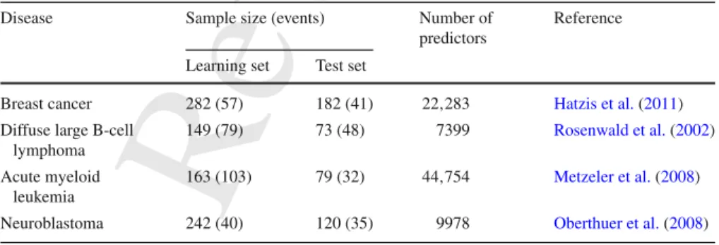
In our analyses, we consider four publicly available medical data sets with survival 225

outcome and information on gene expression of patients (see Table1). Each of these 226

data sets consists of a learning set, using which we compute the optimal number of 227

boosting steps and fit the model, and a test set, for which we compute the integrated 228

Brier score. It is particularly important to keep the learning and test data totally separate 229

in order to have a reliable evaluation of the prediction abilities of the resulting models. 230

In all analyses, we assume that the covariate effects are linear and that the proportional 231

hazards assumption holds. 232

Breast cancer data This data set is from a prospective multicenter study conducted 233

byHatzis et al.(2011) to develop genomic predictors for neoadjuvant chemotherapy.

234

It involves patients with newly diagnosed ERBB2 (HER2 or HER2/neu)-negative 235

breast cancer, for which information is provided on the (possibly censored) distant 236

relapse-free survival time and the gene expressions of 22283 probe sets, which is 237

obtained through the Affymetrix U133A GeneChip. The data set consists of a learning 238

set, containing information on patients who had their biopsy between June 2000 and 239

December 2006, and an independent test set, whose patients had their biopsy between 240

April 2002 and January 2009. Specifically, we use the observations considered inDe 241

Bin et al.(2014b): the sample sizes are 282 patients (with 57 events) and 182 patients

242

Table 1 The four data sets used in our empirical study

Disease Sample size (events) Number of

predictors

Reference

Learning set Test set

Breast cancer 282 (57) 182 (41) 22,283 Hatzis et al.(2011)

Diffuse large B-cell lymphoma

149 (79) 73 (48) 7399 Rosenwald et al.(2002)

Acute myeloid leukemia

163 (103) 79 (32) 44,754 Metzeler et al.(2008)

Revised

Proof

(41 events) for the learning and test sets, respectively. The data are publicly available 243

from the Gene Expression Omnibus, reference GSE25066. 244

Diffuse large B-cell lymphoma The second data set is from the study ofRosenwald 245

et al.(2002) on patients with diffuse large B-cell lymphoma. It contains 7399

gene-246

expression measurements from 240 patients who had no previous history of lymphoma, 247

divided in a learning set (160 patients) and a test set (80 patients). The outcome of 248

interest is the overall survival time. In our paper we use the data set as pre-processed 249

byBøvelstad et al.(2009), which contains the information of only the 222 patients

250

for which the International Prognostic Index is also available. However, we did not 251

consider this predictor in our analysis. As a result of this restriction, the learning and 252

test sets contains 149 and 73 patients, respectively. Due to the presence of censored 253

data, the effective sample sizes are 79 (learning set) and 48 (test set). 254

Acute myeloid leukemia data The third data set contains information on patients with 255

acute myeloid leukemia enrolled between 1999 and 2003 (learning set) or in 2004 (test 256

set) in a multicenter trial of the German AML Cooperative Group (Metzeler et al. 2008). 257

The outcome of interest is the overall survival, defined as the time between study entry 258

and death from any cause. The learning set contains 163 patients, of which 103 died. 259

The data consist of the gene-expression measurements of 44754 probe sets, obtained 260

using the Affymetrix HG-U133 A&B microarray. For the 79 patients belonging to 261

the test set (32 events), instead, the gene expressions were derived using Affymetrix 262

HG-U133 plus 2.0 microarray. The data is publicly available from Gene Expression 263

Omnibus, reference GSE12417. 264

Neuroblastoma data The last data set contains information on patients with neurob-265

lastoma studied byOberthuer et al.(2008). The original learning set consists of 256 266

patients recruited between 1989 and 2004 for the German Neuroblastoma Trial NB90-267

NB2004 for which the overall survival time and the gene expressions of 9978 probe 268

sets are available. The test set consists of 120 patients with the same disease, but col-269

lected in several countries (29 in Germany, 26 in the US, 26 in France, 12 in Spain, 270

11 in Italy, 6 in Belgium, 5 in the UK and 5 in Israel), for which the same outcome 271

and probe sets were measured. In our study, we did not directly use the data from 272

the original study (available from the ArrayExpress database, accession number E-273

MTAB-16), but those pre-processed byBøvelstad et al.(2009), in which 14 patients 274

are excluded due to missing data. Since it was not possible to recover the original split 275

into learning and test sets, here we randomly split the whole data set into a learning 276

set of 242 patients (40 events) and a test set of 120 patients (35 observations), which 277

are the sample sizes used byBøvelstad et al.(2009). 278

3.2 Study design 279

The main focus of our first study is the cross-validation-based choice of the optimal 280

number of boosting steps in model-based and likelihood-based boosting. We consider 281

values between 0 and 200. The lower limit leads to the null model, while the upper limit 282

Revised

Proof

has been arbitrarily chosen as “sufficiently large” (namely, twice the default in both 283

mboostandCoxBoost). We investigate how the variability caused by randomness due 284

to the CV fold-split affects the results of the boosting procedures in terms of number 285

of iterations performed, selected predictors and prediction ability of the models. 286

In our analysis, for both boosting techniques we replicate the following 2000 times: 287

– we apply the 3-, 5-, 10- and 20-fold CV procedures to compute the optimal number 288

of boosting steps, using only the observations from the learning set; 289

– we fit a prediction model by applying the boosting technique to the learning set, 290

using the tuning parameter obtained in the previous point; 291

– we note the number of predictors selected in the model; 292

– we evaluate the prediction ability of the model by estimating the integrated Brier 293

score on the test set. 294

In addition, we collect the same information (number of boosting steps, number of 295

selected predictors, integrated Brier score) when using leave-one-out CV: since this 296

procedure is deterministic, this operation is performed only once. 297

3.3 Results 298

3.3.1 Number of boosting steps

299

The first goal of this empirical study is to evaluate how the optimal number of boosting 300

steps (m_stop) is influenced by the different random splits—learning and test sets—of 301

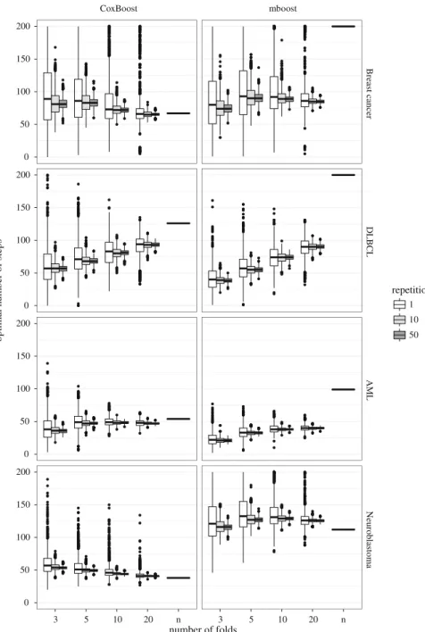
the cross-validation procedure. Figure1shows the distribution of the values obtained 302

over 2000 iterations for each data set, using the CV procedures implemented both in 303

mboostand inCoxBoost. This and the following figures contain information on results 304

of regular CV as well as information on results of repeated CV. The repeated CV is 305

discussed in Sect.4. For now we focus on the white boxplots in Fig.1, which show 306

results for the regular cross-validation. Regardless of the boosting technique chosen, 307

the variability ofmstop is very large, with values that range from 0 (minimum) to 308

200, the upper limit that we considered in our experiment. In particular, this means 309

that, using the same data, we can obtain completely different results simply due to 310

the particular fold-split used. The four considered example data sets suggest that 311

this result may be partially mitigated by a large sample size (although this different 312

behavior may of course also be simply due to random variations): we notice that in the 313

acute myeloid leukemia example, in which we have 103 events, we experience less 314

variability (see Fig.1, third row) than in the other data sets, especially when applying 315

mboost. Nevertheless, it is worth noting that the sample sizes and, more in general, 316

the characteristics of all our data sets, are typical of biomedical studies and therefore 317

in practical situations we may experience this large variability in the choice ofmstop. 318

As expected, the variability decreases with an increase in the number of folds because 319

increasing the number of folds means approaching to (the completely deterministic) 320

leave-one-out CV. Leave-one-out CV produces extreme numbers of steps inmboost

321

for all data sets except the Neuroblastoma data set and forCoxBoostin the DLBCL 322

data set. All extreme numbers of steps for leave-one-out CV are higher than most or 323

all numbers of steps computed by other cross-validation procedures. This suggests 324

Revised

Proof

Fig. 1 Number of boosting steps (mstop) selected in the 2000 iterations (except leave-one out CV) computed

using different CV folds in the four data sets with bothCoxBoost(left) andmboost(right). The color defines the type of CV. White stands for normal, gray for repeated CV

Revised

Proof

that leave-one-out CV leads to models that are more likely to overfit the data in these 325

cases. 326

Note that in our study the number of boosting steps is allowed to vary from 0 327

to 200. In some cases (see, e.g., the results for the breast cancer data set, Fig. 1, 328

first row) the upper limit is reached, meaning that the results could be even more 329

extreme with a larger maximum number of boosting steps. Given the relevant increase 330

in computational time and computer memory necessary to consider a higher upper 331

limit, we think that a value of 200 is fairly reasonable and sufficient to demonstrate 332

the problem of variability induced due to the random CV splits. 333

3.3.2 Selected predictors

334

The high variability in the choice ofmstopis not a problem itself, but it may substantially 335

affect the model building process and consequently the properties of the prediction 336

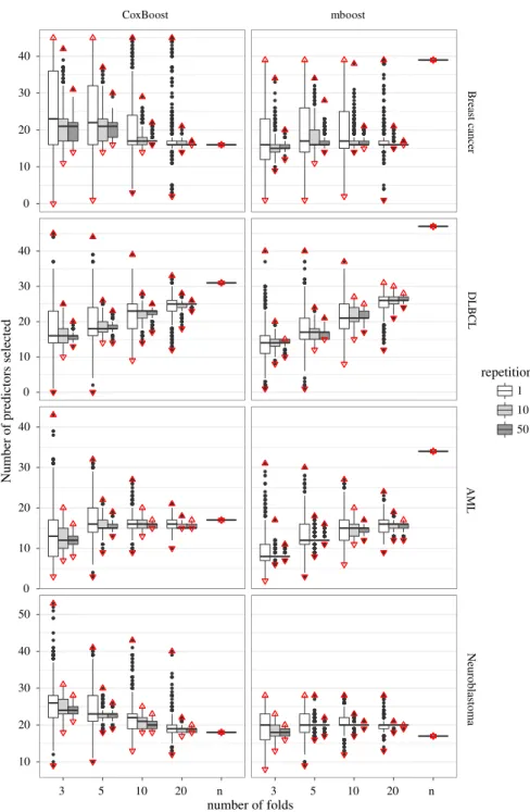
model. In Fig.2we report the number of predictors selected in each of the replications 337

of our experiment for the model-based (mboost) and the likelihood-based (CoxBoost) 338

boosting procedures, respectively. The downward facing triangles indicate the min-339

imum number of predictors selected, i.e. the number of predictors always selected. 340

The upward facing triangles indicate the maximum number of predictors selected, 341

i.e. the number of predictors selected at least once. For a more precise visualization 342

of the number of predictors always selected and the number of predictors selected at 343

least once, see Figures 6 and 7 in the Supplementary Material. The Supplementary 344

materials also contain the complete tables of the selected predictors, including the 345

information on the number of times they are selected (Tables 2–5 in the Supplemen-346

tary Material). Note that the number of predictors selected at least once, the number of 347

predictors always selected and the mean number of predictors selected, is equivalent 348

for leave-one-out CV because it is deterministic and was only computed once. 349

Again, we first focus on the regular CV and ignore the results of the repeated CV 350

for now. The different values of mstop, as determined by the random fold-splits in 351

the cross-validation procedure, greatly influence the prediction models in terms of 352

selected predictors. In particular, extremely low values ofmstopprevent the boosting 353

technique from including many predictors in the model: as a consequence, very few 354

predictors are selected in all 2000 replications performed in our study. On the other 355

hand, high values ofmstopcan result either in higher values for the estimates of a few 356

predictors or in a high number of selected predictors: in our examples the latter seems 357

to happen, as shown by the relatively large number of predictors selected at least once. 358

Note that a boosting model always contains all predictors of a scarcer model (with 359

fewer boosting steps), i.e. the predictors selected in the beginning always stay in the 360

model. 361

The (relatively) greater stability in the choice ofmstopinduced by a larger number 362

of folds in the cross-validation procedure results both in an increase in the number of 363

predictors selected in all replications and a decrease in the predictors selected at least 364

once. This is least strong in the application of the breast cancer data: both formboost

365

andCoxBoost, the variability of mstop slightly decreases with increasing number of 366

folds but not as strong as in the other applications (see Fig.1, first row). This results 367

in a less evident stabilization in the predictors selected. For example usingCoxBoost

Revised

Proof

Number of predictors selected

repetitions 1 10 50 Breast cancer DLBCL CoxBoost mboost

Fig. 2 Number of predictors selected in 2000 iterations computed using different CV folds in the four data sets with bothCoxBoost(left) andmboost(right). The color defines the type of CV. White stands for normal, gray for repeated CV. The triangles indicate the minimum and maximum number of predictors selected (color figure online)

Revised

Proof

the number of predictors always included is 0 for the 3-fold CV, 1 for the 5-fold, 369

3 for the 10-fold and 2 for the 20-fold for the breast cancer data, whereas for the 370

acute myeloid leukemia data it is 3 for the 3-fold, 3 for the 5-fold, 9 for the 10-fold 371

and 10 for the 20-fold CV. The number of predictors selected at least once is always 372

45 for the breast cancer data but goes down from 43 (3-fold) to 21 (20-fold) for the 373

acute myeloid leukemia data. There is no tendency of the median number of selected 374

predictors over data sets. For the DLBCL and AML data it increases with increasing 375

number of folds. For the Breast cancer and Neuroblastoma data it decreases with 376

increasing number of folds for CoxBoost and does not show a clear tendency for 377

mboost. 378

Leave-one-out CV in general tends to favor more complex models, which are more 379

likely to overfit the learning data. Figure2 supports that inmboostfor all data sets 380

except the neuroblastoma data set. ForCoxBoostthe number of predictors selected is 381

particularly high for the DLBCL data. So essentially all examples that show extremely 382

high values formstopalso show many predictors included in the model. 383

Finally, we note that in all the four data sets the rank of the predictors based on 384

their inclusion frequencies is slightly different betweenmboost andCoxBoost (see 385

Tables 2–5 in the Supplementary Material). This is a consequence of the differences 386

in the learning path for the two boosting techniques (for further details, seeDe Bin 387

2016).

388

3.3.3 Connection between the number of boosting steps and the number of selected

389

predictors

390

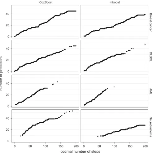
Throughout the paper, we stressed the influence of the number of boosting steps on the 391

model sparsity. To better understand this statement, we plot in Fig.3all values ofmstop 392

obtained inalliterations against the number of predictors included in the corresponding 393

models. Given a certainmstop the model is deterministic and hence a differentiation 394

between different types of CV is not needed here. We note that models are less sparse 395

as the value of the optimal number of boosting steps increases, resulting in a non-396

decreasing function. The steps in the curve correspond to those iterations in which 397

the boosting algorithm includes a new predictor into the model. When the algorithm 398

updates the regression coefficient of a previously selected predictor, instead, the curve 399

remains flat. Please note that the boosting learning path is deterministic. Therefore, 400

once we know the number of boosting steps (and the penalty factor), we can determine 401

uniquely the fitted model. 402

Figure 3 shows once again how important a stable selection of the number of 403

boosting steps is. Extremely large values may result in extremely complex models and 404

the other way around for extremely smallmstop, with obvious implications in terms 405

of interpretation and prediction accuracy. 406

We note that the slopes of the curves formboostandCoxBoostare fairly similar. 407

The largest difference occurs in the Neuroblastoma data set. Here for the most extreme 408

value that we allow formstop, namely 200, the number of predictors is much lower 409

formboost(28) than forCoxBoost(53). Please note that the slopes of the curves are 410

also strongly related to the value chosen for the penalty parameter. The stronger the 411

penalty (i.e., smallerν for mboost, largerλ forCoxBoost, see also De Bin 2016), 412

Revised

Proof

optimal number of steps

number of predictors

Fig. 3 Optimal number of steps plotted against the number of predictors included in the respective model, for bothCoxBoost(left) andmboost(right)

the less steep the curve. Formboostwe usedν =0.1 and for CoxBoostλ =2052 413

for the breast cancer data,λ =1422 for the DLBCL data,λ =1854 for the AML 414

data andλ=720 for the neuroblastoma data. These values were computed using the 415

procedure described in Sect.2.2. Larger values of the penalty parameter correspond 416

to smaller step-wise updates of the coefficients, and consequently there are more 417

iterations without adding new predictors (flat parts of the curves in Fig.3); with a 418

larger penalty it may be necessary to perform two boosting steps to obtain the same 419

coefficient update obtained in one step in case of a small penalty. 420

3.3.4 Prediction ability

421

When we are interested in explanatory models, knowledge of the selected predictors 422

and the stability of the resulting model among several repetitions of the same procedure 423

is particularly important. This is not, however, the main focus of boosting: the boosting 424

Revised

Proof

approach is mainly used in the context of prediction models, where the focus is more 425

on the goodness of the prediction than on the model itself. For example, if we have two 426

strongly correlated predictors, from a predictive point of view it is equivalent to include 427

the former, the latter, or both with two coefficients that combine their effects. For this 428

reason, here we investigate the effect of the randomness of the cross-validation-based 429

choice ofmstopon the prediction ability, analyzing the differences in the estimates of 430

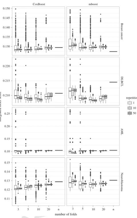
the integrated Brier score among the resultant models. We report in the white boxplots 431

of Fig.4the results forCoxBoost (left) and formboost(right) using 3-, 5-, 10-, 20-432

fold and leave-one-out CV. The results are based on 2000 iterations, except for the 433

leave-one-out CV, for which, obviously, only one value is provided. 434

As a consequence of the decrease in the variability ofmstop, and the relative decrease 435

in the variability in terms of selected predictors, the variability of the integrated Brier 436

score decreases with an increase in the number of cross-validation folds. We note a 437

peculiar behavior in the acute myeloid leukemia example: despite it having the lowest 438

variability in terms ofmstop, it shows a high variability in terms of integrated Brier 439

score, with several cases of extremely high values (visualized by the outlier-points in 440

the box-plots of Fig.4). Strongly unexpected, leave-one-out CV leads to good results 441

formbooston the breast cancer data set. For some unknown reasons in this case the 442

more complex model is the better model. This does not happen often, and may be a 443

particularity of this data set, in which predictors with weak effects are relevant. Note 444

that this result may explain why in the original study a complex gene-signature (up to 445

73 probe-sets) leads to good results, which have not been obtained when focusing on 446

sparse models (see, e.g.De Bin et al. 2014b). Please note that, in general, the inclusion 447

of more predictors decreases the model portability (the model is too specific for the 448

learning data). In this sense, it is not surprising that this result has been obtained by 449

using leave-one-out CV, which is known to favor data-specific models. In all other 450

cases, indeed, the integrated Brier score from leave-one-out CV is higher than the 451

median of the integrated Brier score from other folds, including CoxBoost on the 452

breast cancer data set. 453

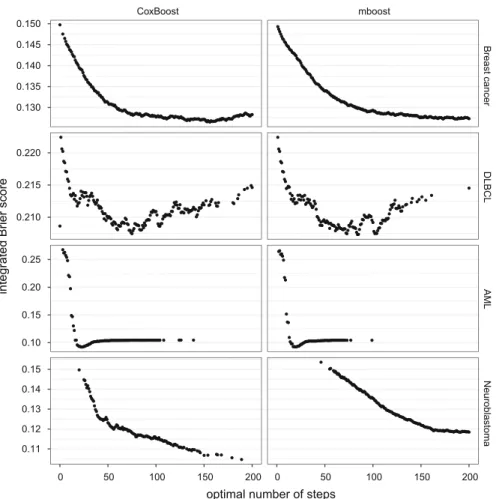
Figure5shows the connection between the number of boosting steps and the inte-454

grated Brier score for all analyses. Again, note that given a certainmstopthe model 455

is deterministic and thus we do not differentiate between types of CV here. For the 456

Breast cancer and the Neuroblastoma data sets the figures suggest thatmstopgreater 457

than 200 should have been chosen, whereas for the other two data sets 200 was more 458

than enough. The figure also gives information on why for the AML data set there are 459

such outliers in the integrated Brier score seen in Fig.4: The prediction performance 460

is very bad if there are only very few boosting steps but improves quickly with an 461

increase in the number of boosting steps. 462

4 Effect of repeated cross-validation

In the previous section we saw that the randomness of the folds split in the cross-464

validation procedure causes variation in the results and the prediction ability. From a 465

theoretical point of view, to avoid this problem we should consider all the combinations 466

of then observations in K folds, following the theory of complete cross-validation 467

Revised

Proof

integrated Brier score

1 10 50

5 3 5

repetitions

Fig. 4 Integrated Brier score for models computed using different CV folds and a different number of repetitions in the four data sets, for bothCoxBoost(left) andmboost(right)

Revised

Proof

optimal number of steps

integrated Brier score

Fig. 5 Optimal number of steps plotted against the integrated Brier score, for bothCoxBoost(left) and

mboost(right)

(Kohavi 1995), and transform the estimator of mstop based on the cross-validated

468

likelihood into a complete U-statistic. With the usual sample size of a medical study, 469

this is clearly computationally unfeasible (see alsoFuchs et al. 2013). Between the 470

current case of only one split and the theoretical case of all splits, nonetheless, there 471

are several intermediate cases in which we can obtain a more stable result in an 472

acceptable amount of time. For this reason, we suggest the use of a repeated cross-473

validation procedure for the choice of the tuning parameter: instead of considering the 474

cross-validated partial log-likelihood, one should consider a repeated cross-validated 475 partial log-likelihood, 476 r cvpl(m)= R r=1 cvplr(m) 477

with R being the number of repetitions and cvplr(m) the cross-validated partial

478

log-likelihood of the r-th repetition. Note that due to the random nature of cross-479

Revised

Proof

validation the subsets D1, . . . ,DK (see Eq. 1) are different for each repetition

480

r=1, . . . ,R. 481

Again, the optimal value ofmstopis computed by maximizing the function overm. 482

4.1 Study design 483

The repeated cross-validated likelihood should be based on the maximum feasible 484

number of different splits, i.e. the largest I that is within the constraints of rea-485

sonable calculation time. In our study, involving 2000 replications of 4 kinds of 486

cross-validation, we considerI =10 as well asI =50. Obviously, when the goal is to 487

fit a prediction model based on a specific sample, a larger number can be considered. 488

The data sets and the methods used in this section are the same as Sect.3. Leave-one-489

out CV is not considered again because the results do not change. We fit a prediction 490

model using the tuning parameter computed in a 3-, 5-, 10- and 20-fold CV procedure 491

and we consider the selected predictors and the prediction ability in terms of integrated 492

Brier score. The procedure is repeated 2000 times. 493

4.2 Results 494

In this section we focus on the impact of repeated CV and with this, also address the 495

parts of the previous figures that were not addressed in Sect.3. 496

4.2.1 Number of boosting steps

497

Figure1shows the improvements in stability in the choice of the optimal number of 498

boosting steps using the repeated cross-validated partial log-likelihood. If we compare 499

the results of repeated cross-validation in gray and normal cross-validation in white, 500

we note a pronounced decrease in the variability, both in terms of interquartile and 501

total range. The decrease between normal CV and the 10 times repeated CV is greater 502

than the decrease between 10 and 50 repetitions. The medians of the distributions are 503

almost equal with a light tendency of being lower when computed with the repeated 504

cross-validated partial log-likelihood. The reason probably lies in the avoidance of 505

the highest values that characterized the distributions in the original cross-validation 506

procedure. The absence of the extreme values (especially those on the borders, namely 507

0 and 200), in particular, is the most positive improvement obtained by implementing 508

the repeated cross-validation, because it prevents situations in whichm_stopis chosen 509

incorrectly due to a particularly unfortunate partition of the observations. 510

4.2.2 Selected predictors

511

The superiority of a more stable choice for the optimal number of boosting steps is 512

clear when examining selected predictors (Figure 7 in the Supplementary Material). 513

Avoiding underestimation and overestimation ofmstop, indeed, leads to the identifica-514

tion of a clear group of relevant predictors always selected in our 2000 replications, 515

and to the decrease of the rarely selected predictors. The latter property is particularly 516

Revised

Proof

evident in the acute myeloid leukemia example, in which the maximum number of 517

selected predictors is 22 when using 10 repetitions and 19 with 50 repetitions. We note 518

that with 50 repetitions we are relatively close to a deterministic result, i.e. the inclu-519

sion frequencies of the predictors is mostly 2000 (always) or 0 (never). The median 520

number of predictors selected barely changes except for the Breast cancer data, for 521

which the median number of predictors selected is lower when the cross-validation 522

is repeated. The complete information on which predictors were selected is shown in 523

Tables 2–13 in the Supplementary Material. 524

4.2.3 Prediction ability

525

The analysis of the integrated Brier score also reflects the advantages of using a 526

repeated cross-validated partial log-likelihood for the choice ofmstop. As can be seen 527

in Fig. 4, the avoidance of extreme values for the tuning parameter results in the 528

disappearance of the worst prediction performances obtained with the simple cross-529

validated partial log-likelihood. For the acute myeloid leukemia example for both 530

mboostandCoxBoostthe bad predictions experienced in the previous section do not 531

occur. The improvement between 10 and 50 repetitions of cross-validation is not as 532

striking as between none and 10 repetitions but with 50 repetitions we come even 533

closer to a stable result, especially for 3-fold CV. To support our findings through 534

Fig. 4 and to analyse the importance of both the number of folds in CV and the 535

number of repetitions, we computed a linear model with the interquartile range of 536

the integrated Brier score as endpoint including main effects of repeated CV and the 537

number of folds. We computed the interquartile range from the 2000 iterations for 538

each method (CoxBoost and mboost), data set, number of folds and number of CV 539

repetitions, which results in 96 values. We computed a separate model for mboost and 540

CoxBoost. The models show that using 10 repetitions instead of 1 has a significant 541

impact whereas using 50 repetitions instead of 10 is not as pronounced for both mboost 542

and CoxBoost (see Table 14 in the Supplementary Material). The more folds are used 543

the lower the interquartile range of the integrated Brier score, but the only confidence 544

interval where both limits are (at least slightly) negative is in the comparison of 5 545

versus 3 folds. The effects estimated from the linear models depend strongly on the 546

four data sets selected. However a simulation study showed comparable results (see 547

Table 1 in the Supplementary Material) which further supports our findings. 548

5 Conclusions

Boosting techniques have proved to be useful tools in selecting a prediction model, 550

especially in the important case in which the number of predictors is much higher than 551

the number of observations. One weakness of boosting is the strong dependence on 552

tuning parametermstop, namely the number of boosting steps. Please note that several 553

statistical methods share this weakness. Until now there has not been a convincing 554

theory developed on the choice of this parameter and practitioners are compelled 555

to use a cross-validation procedure. We have seen that this solution is sub-optimal, 556

since it may lead to surprisingly different results in terms of selected predictors and 557

Revised

Proof

prediction ability of the model depending on the particular partition of the observations 558

into the CV folds. A particularly unfortunate split may cause a severe underestimation 559

or overestimation of the optimal value of boosting steps, with the consequence that 560

the boosting algorithm may produce a very misleading model. We have seen that this 561

problem affects the CV procedure irrespectively of the number of folds used. In our 562

study, we showed that the implementation of a repeated CV procedure decreases the 563

variability in the choice of the tuning parameter and produces a more robust result: as 564

a consequence, far fewer extreme values ofm_stopwould be expected. The results of the 565

10-replication cross-validated partial log-likelihood suggest that few replications are 566

sufficient to greatly improve the selection of the best tuning parameter. The extension to 567

50 replications shows that increasing the number of replications may lead to even better 568

results. As often happens, however, there is no free-lunch solution and an increase in 569

replications also results in a large increase in the number of computations to perform. 570

Therefore, the trade-off between variability reduction and computational time plays an 571

important role in the choice of the number of replications. In our opinion, 10 (or only 572

a few more, let us say 15 or 20) replications may be sufficient to avoid extreme cases 573

and, consequently, obtain reliable results. Nevertheless, we note that the advances in 574

computational techniques (e.g., parallel computing) and computational power (better 575

hardware) constantly relax the computational time issues, and in the future more 576

replications may be implemented without noticeable drawbacks. In this work we 577

focused on boosting for high-dimensional linear Cox-models. We believe that repeated 578

cross-validation will lead to similar improvements in other contexts. Details, however, 579

have to be studied. 580

Acknowledgements We thank Rory Wilson and Jenny Lee for language improvements. HS and RDB 581

were supported by Grants BO3139/4-1, BO3139/4-2 and BO3139/2-3 to ALB from the German Research 582

Foundation (DFG). 583

References

Binder H (2013) CoxBoost: Cox models by likelihood based boosting for a single survival endpoint or 585

competing risks, R package version 1.4.http://CRAN.R-project.org/package=CoxBoost 586

Binder H, Schumacher M (2008a) Allowing for mandatory covariates in boosting estimation of sparse 587

high-dimensional survival models. BMC Bioinform 9:14 588

Binder H, Schumacher M (2008b) Adapting prediction error estimates for biased complexity selection in 589

high-dimensional bootstrap samples. Stat Appl Genet Mol Biol 7:12 590

Boulesteix AL, Richter A, Bernau C (2013) Complexity selection with cross-validation for lasso and sparse 591

partial least squares using high-dimensional data. In: Lausen B, Van den Poel D, Ultsch A (eds) 592

Algorithms from and for nature and life. Springer, Berlin, pp 261–268 593

Bøvelstad H, Nygård S, Borgan Ø (2009) Survival prediction from clinico-genomic models—a comparative 594

study. BMC Bioinform 10:413 595

Brier GW (1950) Verification of forecasts expressed in terms of probability. Mon Weather Rev 78:1–3 596

Bühlmann P (2006) Boosting for high-dimensional linear models. Ann Stat 34:559–583 597

Bühlmann P, Hothorn T (2007) Boosting algorithms: regularization, prediction and model fitting. Stat Sci 598

22:477–505 599

Bühlmann P, Yu B (2003) Boosting with the L₂loss: regression and classification. J Am Stat Assoc 98:324– 600

339 601

Chang YCI, Huang Y, Huang YP (2010) Early stopping inl₂boosting. Comput Stat Data Anal 54:2203–2213 602

De Bin R (2016) Boosting in Cox regression: a comparison between the likelihood-based and the model-603

based approaches with focus on the R-packages CoxBoost and mboost. Comput Stat 31:513–531 604

Revised

Proof

to validation illustrated by two case studies. BMC Med Res Methodol 14:117 606

De Bin R, Sauerbrei W, Boulesteix AL (2014b) Investigating the prediction ability of survival models based 607

on both clinical and omics data: two case studies. Stat Med 33:5310–5329 608

Efron B, Hastie T, Johnstone I, Tibshirani R (2004) Least angle regression. Ann Stat 32:407–499 609

Freund Y, Schapire R (1996) Experiments with a new boosting algorithm. In: Proceedings of the 13th 610

international conference on machine learning. Morgan Kaufmann, pp 148–156 611

Friedman JH (2001) Greedy function approximation: a gradient boosting machine. Ann Stat 29:1189–1232 612

Fuchs M, Hornung R, De Bin R, Boulesteix, AL (2013) A U-statistic estimator for the variance of 613

resampling-based error estimators. Technical Report 148, University of Munich 614

Gerds TA, Schumacher M (2006) Consistent estimation of the expected brier score in general survival 615

models with right-censored event times. Biom J 48(6):1029–1040 616

Graf E, Schmoor C, Sauerbrei W, Schumacher M (1999) Assessment and comparison of prognostic classi-617

fication schemes for survival data. Stat Med 18:2529–2545 618

Hastie T, Tibshirani R, Friedman J (2001) The elements of statistical learning: data mining, inference and 619

prediction. Springer, New York 620

Hatzis C, Pusztai L, Valero V, Booser DJ, Esserman L, Lluch A, Vidaurre T, Holmes F, Souchon E, 621

Wang H et al (2011) A genomic predictor of response and survival following taxane–anthracycline 622

chemotherapy for invasive breast cancer. J Am Med Assoc 305(18):1873 623

Hofner B, Mayr A, Robinzonov N, Schmid M (2014) Model-based boosting in R: a hands-on tutorial using 624

the R package mboost. Comput Stat 29:3–35 625

Hothorn T, Bühlmann P, Dudoit S, Molinaro A, Van Der Laan MJ (2006) Survival ensembles. Biostatistics 626

7:355–373 627

Hothorn T, Buehlmann P, Kneib T, Schmid M, Hofner B (2015) mboost: model-based boosting, R package 628

version 2.4-2.http://CRAN.R-project.org/package=mboost 629

Kohavi R (1995) A study of cross-validation and bootstrap for accuracy estimation and model selection. 630

In: Proceedings of international joint conference on artificial intelligence, pp 1137–1145 631

Mayr A, Hofner B, Schmid M (2012) The importance of knowing when to stop. A sequential stopping rule 632

for component-wise gradient boosting. Methods Inf Med 51:178–186 633

Mayr A, Binder H, Gefeller O, Schmid M (2014a) Extending statistical boosting. Methods Inf Med 53:428– 634

435 635

Mayr A, Binder H, Gefeller O, Schmid M (2014b) The evolution of boosting algorithms. Methods Inf Med 636

53:419–427 637

Metzeler KH, Hummel M, Bloomfield CD, Spiekermann K, Braess J, Sauerland MC, Heinecke A, Rad-638

macher M, Marcucci G, Whitman SP et al (2008) An 86-probe-set gene-expression signature predicts 639

survival in cytogenetically normal acute myeloid leukemia. Blood 112(10):4193–4201 640

Mogensen UB, Ishwaran H, Gerds TA (2012) Evaluating random forests for survival analysis using predic-641

tion error curves. J Stat Soft 50(11):1–23 642

Oberthuer A, Kaderali L, Kahlert Y, Hero B, Westermann F, Berthold F, Brors B, Eils R, Fischer M (2008) 643

Subclassification and individual survival time prediction from gene expression data of neuroblastoma 644

patients by using caspar. Clin Cancer Res 14(20):6590–6601 645

Ridgeway G (1999) Generalization of boosting algorithms and applications of Bayesian inference for 646

massive datasets. PhD thesis, University of Washington 647

Rosenwald A, Wright G, Chan WC, Connors JM, Campo E, Fisher RI, Gascoyne RD, Muller-Hermelink 648

HK, Smeland EB, Giltnane JM et al (2002) The use of molecular profiling to predict survival after 649

chemotherapy for diffuse large-b-cell lymphoma. N Engl J Med 346(25):1937–1947 650

Schmid M, Hothorn T (2008) Flexible boosting of accelerated failure time models. BMC Bioinform 9:269 651

Schumacher M, Binder H, Gerds T (2007) Assessment of survival prediction models based on microarray 652

data. Bioinformatics 23:1768–1774 653

Tutz G, Binder H (2006) Generalized additive modeling with implicit variable selection by likelihood-based 654

boosting. Biometrics 62:961–971 655

Verweij PJ, Van Houwelingen HC (1993) Cross-validation in survival analysis. Stat Med 12:2305–2314 656