How To Analyse Cloud Data Centre Performance

(1)

Workload Generator for Cloud Data Centres

Georgios Moleski - 1103614

School of Computing Science Sir Alwyn Williams Building University of Glasgow G12 8QQ

(2)

Education Use Consent

I hereby give my permission for this project to be shown to other University of Glasgow students and to be distributed in an electronic format.Please note that you are under no obligation to sign this declaration, but doing so would help future students.

(3)

3.6.3 Limitations . . . 15 3.7 Pox . . . 15 3.7.1 Features . . . 15 3.7.2 Components of Interest . . . 15 3.7.3 Limitations . . . 16 3.8 Traffic Generators . . . 16 3.8.1 Iperf . . . 16 3.8.2 D-ITG . . . 17 3.8.3 Netperf . . . 18 3.9 Related Work . . . 18 4 Research Methodology 20 4.1 Project organisation . . . 20 4.1.1 Project Plan . . . 20 4.1.2 Evaluation of Plan . . . 21

5 Workload Generator Implementation and Design 22 5.1 System Overview . . . 22 5.2 Design . . . 23 5.2.1 Programming Language . . . 23 5.2.2 Architecture . . . 23 5.3 User Interface . . . 23 5.4 Implementation . . . 24 5.4.1 DCWorkloadGenerator . . . 24 5.4.2 View . . . 28 5.4.3 Model . . . 28 5.4.4 DCTopo . . . 29 5.4.5 Traffic Generator . . . 30 5.4.6 DCPlot . . . 31 5.5 Limitations . . . 31

(5)

6 Evaluation 33

6.1 User evaluation . . . 33

6.1.1 Feedback . . . 33

6.2 Experiments . . . 34

6.2.1 Fat Tree vs Three Tier . . . 34

6.2.2 Different Links . . . 35

6.2.3 TCP Window Size . . . 36

6.2.4 Server allocation impact . . . 37

6.2.5 Different queue size . . . 38

6.2.6 Protocols . . . 39 6.3 Validation . . . 40 7 Conclusion 42 7.1 Summary . . . 42 7.2 Reflection . . . 42 7.3 Future Work . . . 43

(6)

Abstract

As a result of the demand in Cloud Computing, the number of challenges that need to be overcome in order to improve the performance and availability of the fast growing technology, is significantly increasing. Among those, traffic and workload characterization plays an important role in identifying bottlenecks and mitigating performance degradation.

This project looks to discover more about the traffic characteristics of cloud data centres, by reproducing experiments and examining performance results gathered from reproduced network-wide traffic matrices, con-structed on network-wide and network-level dynamics.

Using Mininet to achieve a realistic virtual network environment and Iperf to handle the end-to-end gen-eration. The software is capable of receiving an application-service traffic matrix and run distributed traffic generations based on the captured communication patterns on a Data Centre network topology and report its performance statistics which can be further analyzed and reviewed.

A number of experiments are included based on different scenarios, to highlight the most important findings and to demonstrate the performance fidelity of the system, by comparing the findings with similar observations found in a number of published research papers.

(7)

Chapter 1

Introduction

Cloud computing is an emerging paradigm that has seen rapid growth over the recent years. Its positive impact in the area of technology and business is the reason enterprises started migrating their applications and services to the cloud. In general, cloud computing is defined as a model which allows the network access to a shared pool of configurable computing resources in a convenient manner with little effort of management or service provider interaction [15].

Data Centre Characteristics:

• Types

– Public Clouds: are owned and managed by third party service providers in which they make resources available to the general public over the internet. Services may be free or on a pay-per-usage model [8].

– Private Clouds: are also owned by a single organisation, however in private clouds the consumers (mostly enterprises) have exclusive use and control over their data [15].

– Hybrid Clouds: are a composition of public and private cloud which remain uniquely separated but are bound together by standardized or proprietary technology [15].

• Availability

– On-Demand: allows users to acquire resources and access their information on demand and any time without requiring any human interaction [15].

– Broad Network Access: allows heterogeneous clients platforms to access resources over the internet through standard mechanisms [15].

– Measured Service: Cloud systems make it so resource usage is transparent to both user and provider (e.g storage, bandwidth, processing) [15].

• Service Models

– Software as a Service (SaaS): where provider’s applications running on a cloud infrastructure are provided to the consumer over various clients (e.g browser) [15].

– Platform as a Service (PaaS): where the consumer is able to deploy and run applications onto the cloud infrastructure which are created using programming languages, libraries or any other tools [15]. – Infrastructure as a Service (IaaS): where fundamental computing resources (e.g storage, processing) are provided to the consumer making it possible to deploy and run any software including operating systems [15].

(8)

Cloud computingarchitectureconsists of two main components known asfront endandback endplatforms [15]. The front end refers to the client part of the cloud computing platforms. This is typically the device that the end users interact with to manage and access their information. Client falls into three categories known as the mobile (mobile devices e.g smartphones), thin (client without internal hard drivers and rely on servers) and thick (regular computers which use browsers). The back end consists of a collection of remote servers which make up the known Cloud Data Centres.

Cloud Data Centre [19] which is the main focus of this project, refers to any large, dedicated cluster of computers that is owned and operated by a single organization. Data centres usually act as centralized repositories used for the storage, management, and dissemination of data and information. In cloud computing a single or multiple distributed data centres may be used depending on the scale of services provided which may range from thousands to ten thousands.

1.1

Overview and Motivation

Even though Data centres have been around for a while few publications were made available in regard to the nature of their traffic, therefore little is known about the network-level traffic characteristics of current data centres. What has been already observed from the released traffic matrices is that traffic in Data Centres can be unpredictable /citevl2 and bursty in nature [20] which makes it difficult to find novel mechanisms and protocols that can adapt and cope with its highly divergent nature [2].

The purpose of this project is to build distributed traffic generator which will be able to accept an application-service level traffic matrix as an input and construct the network-wide and network-level dynamics that will allow the reproduction of a network-wide traffic matrix object. Simply put, the application receives a real traffic matrix containing information only about the services and the communication patterns (e.g how many services communicate and how many bytes are exchanged) see Figure 5.1 and nothing about the underlying network environment and from the data obtained from the traffic matrix it dynamically constructs the network layer parameters for the whole data centre and generates traffic distributed to all the communicating pairs.

The software during and after each traffic generation, gathers information about the monitoring and traffic generation results and reports the output which can then be plotted and examined to find trends and identify any bottlenecks that may be responsible for the Data Centre’s performance issues.

1.2

Report Outline

The remainder of this document will discuss the following:

• Background and Related Work. This chapter will give a review about the literature used and the back-ground research conducted.

• Requirements.This chapter discusses the initial and final requirements.

• Research Methodology. This chapter will provide details of the research strategy and project planning and organization approaches.

• Workload Generator Implementation and DesignThis chapter will detail the process used to design and implement the software system.

• Evaluation This chapter will detail the process used to evaluate the system’s performance accuracy by listing some of the experiments conducted as well as the validation of the tools used.

(9)

• Conclusion and future workThis chapter will give a brief summary and a reflection of the project in general. Finally some of the future plans will be discussed.

(10)

Chapter 2

Requirements

The chapter discusses how requirements evolved to a more specific and refined version from the initial high level abstract requirements given at the end the reasoning of why some modification and choices were made.

2.1

Abstract requirements

The requirements were detailed from the beginning outlining which were the core requirements and what op-tions could serve as the potential environment and technologies that could be used to aid the implementation of the system. This section discusses the high level abstract requirements that the software needed to fulfil and implement.

The abstract requirements were as follows:

• Accept Traffic Matrix as input. A traffic matrix as explained in more detail in the Background section captures the bytes exchanged between a pair of services over a period of time. The software is expected to read such file, parse the data and store relevant information about the cloud data centre services and their communication patterns.

• Set up network topologies. Based on the data gathered from the traffic matrix, the software should be able to initiate the right number of Virtual Machines and set up a Cloud Data Centre network topology. • Generate traffic. Since the main purpose of this project is to build a traffic generator, being able to

generate traffic is a fundamental requirement. The traffic generation needs to run in parallel and distribute the traffic to the whole Data Centre so that all servers in the network topology can generate at the same time and the network-wide traffic matrix object can be reproduced accurately.

• Playback the captured communication patterns.Which means that the system must be able to accept the given application-service level traffic matrix and construct the network-wide and network-level dynamics of the Data Centre that are used to reproduce the network-wide Traffic Matrix object.

• Reproduce experiments.Since the main purpose of this project is to be able to characterise the behaviour of Cloud Data Centres and identify bottlenecks, experiments are essential and can be reproduced by exam-ining the output performance statistics.

Along with the requirements, the following platform and language choices were suggested: Platforms: Linux, Mininet

(11)

2.2

Refined Requirements

During the course of the system implementation some of the requirements evolved into a more refined version of the abstract requirements given at the start. This doesn’t mean that extensive changes were made, but additional information was provided on what the system was required to do in detail. All the additions and modification were discussed with the supervisor before being adopted.

According to the refined requirements the system is required to:

• Run in a Mininet network environment. Mininet is easy to use and provides flexibility in managing and extending its components.

• Read additional information from a traffic matrix file including the service ID and how many servers are in each service.

• Dynamically scale the number of services to emulate with smaller or larger topologies.

• Support at least two Data Centre topologies. More complex would be hard or impossible to emulate. • Support UDP and TCP traffic generation.

• Use an already existing traffic generator such as D-ITG or Iperf. As discussed with the supervisor, using existing traffic generator would make the implementation end faster, possibly yield more accurate perfor-mance results and allow extended protocol tuning (TCP window size, UDP bandwidth rate).

• Report overall performance which includes throughput, packet loss and duration. • Monitor link utilisation.

• Plot the performance results on a graph.

• Conduct experiments by running the system under different parameters and configurations and analyse the performance statistics and plots to identify trends and bottlenecks.

2.3

Non-functional Requirements

The non-functional requirements are used to specify the quality and performance of the system. Non-functional requirements were not listed in the project specification, however a number of operational requirements where set that are necessary for the system in order to be usable and consistent. Therefore it has been decided that the following Non-function requirements should be found in the system:

• Be able to construct a Data Centre topology of at least 100 serversMininet can emulate several hundred nodes in total, therefore by having at least 100 servers the system will be able to cover significant areas of the traffic matrix file.

• Overall Data centre emulation should take no more than 5 minutes. This requirement highly depends on Mininet, however the system should not make it any slower.

• Usable for experiments and common userTherefore a user interface should be included as well as the ability to run it quickly by passing the parameters as command line arguments.

(12)

Chapter 3

Background and Related Work

The following chapter provides a background on the dominant design patterns for Data Centre network archi-tectures and the characterisation of the traffic which propagates them. An overview of Mininet, the environment used to simulate the Data Centre architecture will also be given along with some details of the Iperf traffic generator and its accuracy.

3.1

Data Centre Architectures

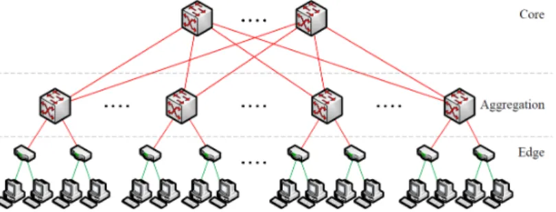
Cloud Data Centres typically consist of tens to thousands of servers all of which concurrently support a variety of services. As explained in the VL2 [2] research paper, a typical data centre physical topology maintains a hierarchical structure with a bottom layer of servers connected with edge switches also known as top-of-rack and a top layer consisting of core switches all of which are interconnected with a middle level layer consisting of aggregation switches. Each rack in the topology contains about 20 to 40 servers depending on how large the data centre is and each router is connected to an edge (Top of a Rack) switch with a 1Gbps link, even though recently data centres started upgrading their links to greater speeds (e.g 10gbps). The hierarchical structure described above is also known as a clos topology and it is designed to be three staged involving an ingress stage, a middle stage, and an egress stage. The most common data centre topology is the canonical 3-tiered topology which inherits all the properties discussed above, consisting of the edge tier, the aggregate tier and the core tier and connects the data centre to the WAN as shown in Figure 3.1. In small data centres, it is common to have the core tier and the aggregate tier merged into one tier resulting in a 2-tiered data centre topology [20]. Even though the three tiered canonical tree is used by many data centres, a great proportion of those started shifting to a special instance of a clos topology called a fat-tree [11]. A fat-tree topology as shown in Figure 3.2, consists of k-pods which essentially classify the size of a k-ary fat-tree and contain one layer of k/2 aggregate switches and one layer of k/2 edge switches. The edge layer switches are usually connected directly to (k/2)2 hosts and the aggregate layer switches are connected to (k/2)2 core switches. In general, a fat-tree built with k-port switches supports k3/4 hosts.

(13)

Figure 3.1: Three Tier Canonical Network Architecture

3.1.1 Canonical Tree vs Fat tree

When it comes to the canonical Tree topology and the Fat tree topology one of their key difference is that Fat trees have way more links connected to all levels of the tree topology compared to the canonical tree, which is essentially where its name is taken from. This makes the cost and complexity of the fat tree higher since there will be more switches and more links. However as argued in a paper about the complexity of tree-like networks [5] fat-trees are often chosen to achieve low latency, high bandwidth and high connectivity interconnected networks for parallel computers. Another key advantage of fat trees is the high availability of paths due to having multiple links. High availability as stated in the paper [5] increases the performance rate for all kinds of workloads independently of their spatial, temporal or size distributions. However, one important issue in fat-trees is locality in parallel applications. It is a common practice that parallel applications arrange their processes to be as close as possible so that in case their processes are communicating, the locality in communication can be exploited. It appears that fat-trees do not take into account locality and as stated in the paper [5] performance degradation is depended on the scheduler. If a scheduler does not guarantee assignment of resources to neighbor processes then locality is not an issue. However topology-aware schedulers that schedule applications consecutively will have performance issues in fat-tree topologies and according to the paper [5] using a topology-aware scheduler on fat-trees will cause under-utilisation of the upper levels of the topology. To conclude, fat-trees perform overally better than the canonical trees, however in terms of cost and complexity the canonical tree is considered a better choice and if locality is considered it can perform better than fat-trees in some cases.

(14)

3.1.2 Advanced Topologies

In this section four more sophisticated network architectures are discussed that use more advanced algorithms and structures in order to achieve optimal performance.

DCell

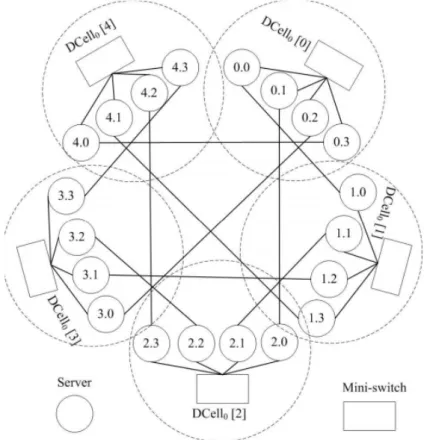
DCell as illustrated in Figure 3.3 is a recursively defined structure which works by having multiple instances of its self where a high-level DCell is recursively constructed from many low level DCells all of which are fully connected with one another forming a fully-connected graph [3]. At the level of servers there are multiple links connecting different levels of DCells to each server. In detail servers are connected to other servers and mini-switches which are used in DCell to scale out doubly exponentially with the server node degree. The main advantage of using such architecture is fault tolerant since it does not have a single point of failure. Also in the DCell paper [3] it is stated that DCell provides higher network capacity than the traditional clos topologies for various types of services. One important trade-off in DCell are the high costs due to expensive core switches and wiring since it uses more and longer communication links than the clos topologies.

Figure 3.3: DCell Network Architecture

BCube

Bcube exchibits a server centric design [4] which uses commodity servers and commercial-off-the-shelf switches. As shown in Figure 3.4, each server connects to mini-switches and is fault tolerant. In addition, Bcube is load balancing and it significantly accelerates representative bandwidth intensive applications. Lastly, as mentioned Bcube offers graceful performance degradation as the server and/or switch failure rate increases.

(15)

Figure 3.4: BCube Network Architecture

VL2

Virtual Layer 2 (VL2),is a network architecture [2] which uses flat addressing to allow services to be placed anywhere in the network, Valiant Load Balancing for traffic spreading across network paths, and address resolu-tion which supports scaling to large server pools, without adding complexity to the network control plan. Some of the key advantages in adopting VL2 are the path diversity, the elimination to the need for oversubscription and any the ability to have any service assigned to any server, while maintaining uniform high bandwidth and performance isolation between services. The most important aspect in VL2 however is its simple design that makes it possible to be implemented on existing hardware without making changes to switch control and data plane capabilities.

Monsoon

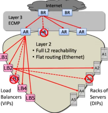
Monsoon as seen in Figure /refmonsoon is a mesh-like architecture [1] which uses commodity switches to reduce costs and allows powerful scaling to a significant number of servers. In Monsoon, Ethernet layer 2 is used to eliminate server fragmentation and improve cost savings and IP layer 3 is used for dividing requests from Internet equally to access routes by Equal Cost MultiPath (ECMP). Lastly, Valiant Load Balancing is used to increase performance.

3.2

Traffic Analysis

The accuracy and correctness traffic analysis highly depends on the methods used to gather the relevant traffic data. The three common methods used areSNMP counters,Sampled flowsandDeep packet inspections.

SNMP counters: are data gathered from individual switch interfaces and provide information about packet and byte counts. The concerns about this methodology is the limited availability to coarse time-scales restricted by how often routers can be polled. Another issue is SNMP provides limited information on flow-level and host-level behaviour [17].

Sampled flows:[17] are used to provide flow level insight at the cost of dealing with higher volume data for analysis and for assurance that samples are representative. Fortunately, newer platforms increase the availability on the above capabilities.

(16)

Figure 3.5: Monsoon Network Architecture

Deep packet inspections: involve a method known as packet filtering which examines the data part of a packet as it passes an inspection point [17]. Research effort are made to mitigate the cost of packet inspection at high speed, however this is not supported by many commercial devices.

The most common observations made about the behaviour of traffic is that the majority of traffic originated by servers(80%) stays within the rack [wild] and in general the ratio of traffic entering/leaving a data centre is 4:1. In addition, servers inside the datacenter have higher demands for bandwidth than external hosts. Lastly, the network is bottleneck to computation which are a result causes ToR switches’ uplinks to go above 80% of utilisation [2].

From measurements conducted by Greenberg et al. [2] it is found that traffic patterns inside data centres are highly divergent and change rapidly and unpredictably. This means that traffic changes nearly constantly with no periodicity that could aid in predicting the future. Consequently, this makes it hard for an operator to engineer routing as traffic demand changes. As a result, randomness is used to improve the performance of data centre applications.

3.2.1 Flow characteristics

In terms of flow characteristics in Data centres, it is indicated that the majority of flows are small ( also described as mice) and are only a few KB which are resulted from hellos and meta-data requests to the distributed file system. Longer flows can have sizes ranging from 100 MB to 1GB and it is assumed that 100MB which make the majority of long flows are file chunks broken by the distributed file system while GB flows are rare [2].

Internet flows exhibit the same characteristics of being small, however the distribution is simpler and more uniform in the Data centres. According to Greenberg et al. [2] in Data Centres efforts are made in maintaining an engineered environment driven by careful design decisions and the use of storage and analytic tools. Thus, internal flows originating from such environment, are more likely to achieve simplicity and uniformity.

(17)

network with 1,500 monitored machines, more than 50% of the time an average machine has about ten concurrent flows. However at least 5% of the time it can reach more than 80 concurrent flows but almost never go beyond 100 concurrent flows.

3.3

Traffic Matrix Analysis

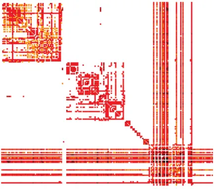
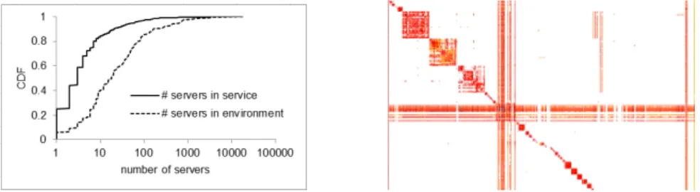
As illustrated in Figure 5.1 a traffic matrix is used to represent how much traffic is exchanged from the server denoted by the row to the server denoted by the column. Usually, the values in traffic matrices denote how much data are exchanged in different intervals which in data centres some common intervals could be 1s,10s and 100s. In the paper discussing bandwidth-constraint failures [tm] the traffic matrix illustrated in Figure [6] consists of service i and j pairs where the total number of bytes transmitted between the service pair R(i,j) is computed and also the total traffic generated by individual services T(i) can be seen at each row. Additionally the traffic matrix is visualised as a heatmap where color is used to denote the amount of communication exchanged from light (small or no communication) to dark (large amount of data exchanged).

Figure 3.6: Traffic Matrix

3.3.1 Workload patterns

The mos common observations in traffic matrices are the workload patterns that can be examined and analysed in order to determine the nature and constistency of the traffic. One observation that can be deduced by just looking at the traffic matrix in Figure [6] is that it isextremely sparse[tm] which means that a small percentage of services communicate. According to the paper [6] out of all possible services only 2% service pairs exchanged data while the remaining 98% do not communicate at all. By taking into account the 2% of service pairs that do communicate it is found that the communication pattern is textbfextremely skewed. In the paper [6] this is reasoned by stating that 4.8% of service pairs generate 99% of all traffic and a 0.1% of those (including services talking to themselves) generate 60% of all traffic. In terms of individual services, 1% of them generate 64% of traffic and 18% of services generate 99% of traffic. Having those percentages can aid in improving the fault intolerance by spreading the services that do not require significant bandwidth across the data centre

(18)

A paper by Benson et al. [wild] provides an insight on the nature of communication patterns by taking into account the different types of applications including Web services, Map Reduce and custom application employed in 10 different data centres split into three different categories which are namely university, private and cloud data centres. The patterns discovered exhibit an ON/OFF nature especially in the edge switches and the durations can be characterised by heavy-tailed distributions. In addition, the nature of traffic is considered bursty which as a result there is an impact on the utilisation and packet loss on the links at every layer of the topology.

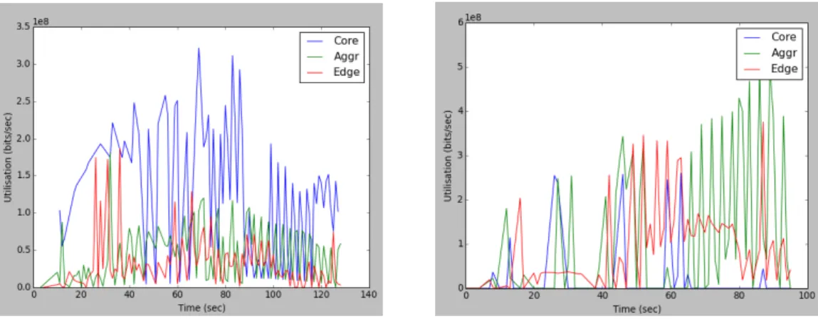
3.3.2 Link Utilisation

Link utilisation in network topologies refers to the bandwidth that a traffic stream takes from the total link capacity. More specifically, utilisation is the number of bits on the link at time x divided by the total bits the link can contain. A common observation that holds for most of the cloud data centres is that utilizations within the core layer links are higher compared to aggregation and edge switches. High utilisation is one of the major causes of congestion in Data Centres and in core links this happens often. In kandula et al. [nature] it is found that out of 1500 monitored machines machines, 86% of the links undergo congestions lasting at least 10 seconds and are caused due to high demand from the application. A 15% of the links go through longer episodes of congestion lasting at least 100 seconds and those are found to be localised to a small set of links. It appears however, that high utilisation is not always directly related to congestion and losses and when losses are found in lightly utilised links the cause is most likely the bursty nature of the traffic in Data centres.

3.4

Data Centre application Types

A paper by Benson et al. [wild] conducted a measure analysis by employing packet trace data and using Bro-Id to aid classify the types of applications on a number of different data centres. The types of data centres used in the analysis involve university campus data centres and a private enterprise data centre. As illustrated in Figure 8 there are four bars for the same private data centre (denoted as PRV2) and the rest of the bars represent three different university campus data centres. Each bar is partitioned in different patterns represent the type of application used in each data centres and the percentage of network traffic that each application is involved to. As observed from Figure 8 the majority of applications in university data centres are web services and distributed file system while the private data centre involves custom applications (denoted as OTHER) proportion of File and Authentication Systems. This is no surprise considering that in university data centres most of traffic (40-90%) leaves the rack and traverses the network’s interconnect while in the cloud data centres the majority of traffic (80%) stays within the rack

3.5

Issues and Challenges

Some of most common issues observed in most data centres are:

• Poor Reliability: This results especially in tree-like topologies where if one of edge switches fail it doubles the load on the other. This may cause unexpected utilisations and congestions that may affect the rest of the network topology and consequently resulting in performance degradation. Some of the advanced architectures discussed above counter this issue by supporting fault tolerance and load balancing.

• Oversubscription in higher layers: It is observed, especially in clos tree-like topologies that over-subscription increases in the higher layers of topology. Servers in the same rack usually subscribed by

(19)

factor 1:1. Links connecting edge (ToR) switches with aggregates are subscribed by factors ranging from 1:5 to 1:20. Core routers which sit at the highest layer of a tree topology are found to be oversubscribed by factors of 1:80 to 1:240 [2]. As claimed by greenberg et al. [2] this leads to fragmentation of resources by preventing idle servers from being assigned to overloaded services, and the entire data centre performance suffers severely as a result.

• Collateral damage: is caused when overuse by one service affects others. Even though a data centre can host up to thousand services there are no any significant mechanism to prevent traffic flood in one service from affecting the others around it [2]. As a result services in the same network sub-tree are doomed to suffer from collateral damage.

• Under-utilisation: is occurred when there are multiple paths and only one of them is used regardless if it is highly utilised. The same issue also exists in servers [2] where resource fragmentation is constraint result in unmet demands elsewhere in the data centre.

(20)

3.6

Mininet

Mininet is a network emulator which is able to simulate a realistic virtual network, running real kernel, switch and application code on a single machine (virtual machine, cloud or native) in a short amount of time.

3.6.1 How it works

Mininet host behaves just like a real machine; it provides options such as using ssh to remotely access it and run arbitrary programs including anything that is installed on the underlying Linux system.

In terms of network emulation, it runs a collection of end-hosts, switches, routers, and links on a single Linux kernel and uses lightweight virtualization to make a single system look like a complete network, running the same kernel, system, and user code.

Programs running in Mininet can send packets through what seems like a real Ethernet interface, with a given link speed and delay. Additionally, when two programs are acting like client and server (e.g Iperf) and communicate through Mininet, the measured performance should match that of two slower native machines. Packets traversing a Mininet network get processed by what looks like a real Ethernet switch with a given amount of queueing.

To sum up, Mininet can emulate real network nodes using software rather than hardware and for most of the part the emulated nodes retain similar behaviour traits to discrete hardware elements. This makes it possible to create a Mininet network that resembles a hardware network, or a hardware network that resembles a Mininet network, and to run the same binary code and applications on either platform.

3.6.2 Benefits

Fast network emulations. It only takes a few seconds to start up simple network making it easy to run, modify, debug or run experiments on it in a short amount of time.

Customisable network topologies.Which gives extreme flexibility on what to simulate. Different users may simulate different topologies for different purposes. For example a single user may simulate single switch topology for a house or companies and researchers may simulate larger Internet-like topologies and data centres Running real programs. Which means anything that runs on Linux is available anyone to run. This gives the flexibility of running commercial monitoring applications or create custom applications that can be used to test or extend the simulated network.

Packet forwarding customisation.OpenFlow protocol is used on Mininet switches therefore custom Software-Defined Network designs that run in Mininet can be transferred to hardware OpenFlow switches for line-rate packet forwarding.

Portability.Mininet can be run on a laptop, server, VM or even on Cloud.

Easy to use. Simple Python scripts can be written to create and run Mininet experiments. Open Source Code.Which gives the ability to reuse, extend or improve.

(21)

3.6.3 Limitations

Resource limitsCPU resources of the system simulating the network need to be balanced and shared among the network nodes.

Single Linux kernel for all virtual hostswhich means that software which depends on BSD, Windows, or other operating system kernels cannot run.

Controller variety. Mininet does not provide a large pool of openflow controllers therefore if additional features are needed or custom routing; then the controller needs be written by the user with the required features. Isolation from Lan and Internet.This limits accessing resources found on the web. However extra config-uration can enable Mininet to connect to the Internet.

By default all Mininet hosts share the host file system and PID space. Therefore care is needed in case there are daemons that require configuration are running and user needs to be careful not accidentally kill any wrong processes.

Timing measurements are based on real timewhich means that faster than real time results (e.g. 100 Gbps networks) cannot be easily emulated.

3.7

Pox

POX is an open source development platform for Python-based software-defined networking (SDN) control applications, such as OpenFlow SDN controllers. It provides components for interacting with OpenFlow switches and framework features for writing custom OpenFlow controllers [10].

3.7.1 Features

• Provides SDN debugging, network virtualisation, controller design, and programming model • Reusable sample components for path selection, topology discovery.

• Portable, running almost everywhere as long as there is Python Interpreter • Provides components for topology discovery

• Supports the same GUI and visualization tools as NOX

3.7.2 Components of Interest

The components below are used to prevent the broadcast storms phenomenon observed in loop topologies (e.g Fat tree) and to provide alternate methods for topology discovery and path selection.

• Forwarding l2 multi: is a component acting as a learning switch which is used in conjunction with openflow discovery to learn the topology of the entire network. As soon as one switch learns where a Mac address is the rest do so as well.

(22)

• OpenFlow discovery:sends LLDP messages out of OpenFlow switches so that it can discover the network topology. It also outputs events about the state of the links (detected, timeout, down) and ports.

• Openflow Spanning Tree:is used with the openflow discovery component to build a view of the network topology and construct a spanning tree on the topology. To avoid broadcast storms it disables flooding on all ports as soon as a switch connects and prevents altering of flood control until a complete discovery cycle has completed.

3.7.3 Limitations

• Openflow discovery has link timeouts which do not work well with large topologies taking significant time to set up. Also LLDP messages sometime do not reach every node causing packet losses.

• Openflow spanning tree may sometimes not pick the shortest path (e.g possibly openflow discovery fails to reach some links). Also using spanning tree some available paths are not used at all.

3.8

Traffic Generators

This section discusses about potential traffic generators that were considered good candidates to be used in the application. At the end Iperf was chosen and to verify its accuracy, additional research was conducted to verify that.

3.8.1 Iperf

Iperf is a simple but powerful tool originally developed by NLANR/DAST for measuring performance and troubleshooting networks. It can be used to measure both TCP and UDP bandwidth performance by allowing the tuning of various parameters and UDP characteristics [9]. Iperf is able to generate traffic on either TCP/IP or UDP and report the bandwidth, delay, jitter, datagram loss.

Iperf uses the client-server architecture which needs to be at the opposite ends so that client can generate traffic and server can receive it. Once the generation is completed, both client and server report the performance results based on the protocol used.

Features and Parameter Options

Iperf gives the possibility to generate traffic and measure the performance throughput using a variety of parame-ters and features which can be general or protocol specific.

In general, the user can specify the port (-p) used to receive and send traffic, the interval time (-i) between periodic performance reports, the length of the buffer (-l) which counts as the datagram size for UDP and the number of times (-n) to transmit the specified or default buffer. In terms of TCP window size (-w) can be set which specified how many bytes to send in one go before requesting for ACKs. The MSS/MTU size (-M) can be set or reported (-m) in addition to the observed read sizes which often correlate with the MSS. In UDP, the bandwidth rate must be set (-b) to specify the desired bandwidth used to send the datagrams.

Iperf has more features which involve parallel running, how much time to generate and other more. Those however are not used in the project therefore they are omitted.

(23)

Accuracy

For generating traffic, Iperf uses the Berkeley sockets through the C API and measures the time it takes for the bytes to reach their destination. Even though Iperf is one of the most popular traffic generators freely available on the Internet, little is known about its accuracy in performance reporting.

A paper published by InterWorking Labs [7] evaluates Iperf’s reporting accuracy in terms of throughput tested in UDP. The observed results were that Iperf was under reporting the actual bandwidth of the link. In addition, the throughput report error was increased as the packet size was reduced. It was then stated that the reason of the bandwidth error report was that Iperf measures the transport level bandwidth. This means that it measure the number of TCP and UDP data bytes carried without taking into account the lower network layers, namely Ethernet, IP, UDP/TCP.

By adding the frames and headers of the missing protocols it concluded that in large packets the under report is minimal where if the packet has little data reporting error goes over 40%.

The paper provides a formula which adds up the unaccounted protocol headers and recalculates the reported Iperf bandwidth into the actual bandwidth.

The formula is: A = ((L + E + I + U) / L) * R

where: A: is the actual link bandwidth in bits/second.

L: is the value given to Iperf’s -l parameter. See Iperf section 3.7 E is the size of the Ethernet framing.

I is the IPv4 header size. U is the UDP header size.

R is the bits/second value reported by Iperf.

At the end it is concluded that Iperf’s reported throughput values are not incorrect but rather used to represent transport level bandwidth and not the raw bandwidth of the link.

3.8.2 D-ITG

D-ITG is a distributed Traffic Generator capable of generating traffic at packet level and accurately replicating appropriate stochastic processes for both IDT (Inter Departure Time) and PS (Packet Size) random variables (exponential, uniform, cauchy, normal, pareto, etc) [18]. Compared to Iperf, D-ITG is capable of generating traffic at network, transport, and application layer and it supports both IPv4 and IPv6 traffic generation and it.

D-ITG has three components, the server instance ITGRecv which receives traffic, the client instance ITGSend which sends traffic and ITGDec instance which store the generation logs. send the traffic.

As it seems D-ITG is a very flexible tool to run on its own and provides a wide range of traffic generation statistics, however it is hard to run inside an application because of the redundancy of components and it does not output the performance results on the command line making it inconvenient to gather results at run time for many parallel generations.

(24)

3.8.3 Netperf

Netperf is a benchmark that can be used to measure the performance of many different types of networking [6]. It provides tests for both unidirectional throughput, and end-to-end latency. The primary focus in using netperf is sending bulk data and measure the performance using the either TCP or UDP Berkeley Sockets interface. Furthermore as stated in the official website netperf supports unidirectional data transfer over IPv4 and IPv6 using three interfaces. The Sockets interface, the XTI interface and the DLPI interface for Link-Level.

Even though netperf seems very powerful tool, it seems to be inconsistent in its reports when being tested against traffic generators. Also there is little documentation on how to fully exploit its features and its byte transfer is not as consistent as it should be.

3.9

Related Work

In this section related software applications are discussed which mainly involve building and testing data centre topologies on Mininet.

• Maxinet: is a system application which looks to achieve distributed emulation of software-defined net-works that consist of several thousand nodes [16]. Using Mininet the maximum number of nodes that can be achieved are several hundred. To extend that number to several thousand it spans the emulated network over several physical machines which establish communication through ssh. To test the performance of such large networks a traffic generator is also provided for generating traffic to a data centre topology. Moreover synthetic traffic matrices are used to regenerate traffic similar to data centres. The system was able to emulate a data centre of 3200 hosts using 12 physical machines. However using such a system can be costly since as stated in the paper more than 10 physical machines powerful machines are needed to emulate a network of over thousand nodes and a slower machine can become a bottleneck for the rest. Therefore such system is powerful but not realist for limited resources.

• Mininet Hi-Fi: is a container-Based Emulator [14], which enables reproducible network experiments using resource isolation, provisioning, and monitoring mechanisms. [repr] The emulator was used on Hedera and DCTCP both designed to conduct experiments and devise novel network algorithms for data centres.

• Hedera: is dynamic flow scheduler for data centre networks, presented at NSDI 2010 which looks to im-prove Equal-Cost Multi-Path (ECMP) routing by proposing a solution for avoiding has collisions between large flows [12] [14]. To evaluate the performance of the data centre in a virtual software environment, with the aid of Mininet HiFi Hedera is generating traffic to measure and compare throughputs achieved by ECMP and a ”non-blocking” network. For the purpose of the experiment a k = 4 Fat tree topology was used with 1Gb/s links and 20 different traffic patterns which are used by a traffic generator program. The results proved to be similar to those observed in a hardware environment, however the experiment parameters had to be scaled down (e.g bandwidth links) as virtual hosts lacked CPU capacity making them unable to saturate their network links.

• DCTCP: Data-Center TCP is an experiment which was suggested in SIGCOMM 2010 as a modifica-tion to TCPs congesmodifica-tion control algorithm [13] [14]. The goal was to achieve high throughput and low latency simultaneously. Similar to Hedera, Mininet-HiFi was used to emulate the experiment in a software environment and compare the results to those obtained in a hardware environment. For the experiment a simple topology of three hosts was used connected to a single 100Mb/s switch. As observed in Hedera the performance fidelity is better when using 100Mb/s, however when using 1Gb/s links the scheduler falls behind.

(25)

By looking to related works trying to simulate experiments and traffic generations to data centres, it is concluded that no system is perfect. Maxinet looks to be the most ideal of all however it requires costs that can’t be covered by everyone. In terms of Hedera and DCTCP using Mininet-HiFi it seems that the Mininet limitations still persist in terms of link capacity and the simple topologies used would most likely miss any behavior and patterns of the traffic found in wider areas of the traffic matrix file.

(26)

Chapter 4

Research Methodology

This chapter outlines the research methodology used to attain some of the background knowledge related to the project and Cloud Data Centres. Project planning and organisation are also discussed highlighting what methods were used and how deliverables were determined.

4.1

Project organisation

4.1.1 Project Plan

To be able reproduce experiments and characterise the behaviour of Data Centre based on an application level traffic matrix, the research must be conducted with precision and information extracted must be accurate in order to get meaningful results. Therefore a significant time was dedicated in researching before and while implementing the software system.

The project was organised into the follow stages four phases:

• Literature review. involved reviewing and understanding the scope and general context of the project. Papers about Cloud Data Centres [15] [19] as well as Traffic Matrices and Traffic Engineering were re-viewed first to familiarise with the topic as it was new to me. Then research papers of related work were gathered and researched so as to help understand the motivation and procedures used and gain a wider view of the topic at hand.

• Detailed Background study. Basic knowledge of Data Centres was not enough for reproducing precise experiments. To be able to construct the network-wide and network-level dynamics, it was essential to understand in detail the properties of both the Data Centre and its Traffic. First the research started by gathering research papers from the project supervisor and his colleagues and the main focus was research-ing the characteristics of a Data Centre Environment (e.g size, architectures, network properties, issues etc) and its traffic (e.g size, duration, patterns etc). Then since the traffic matrix had limited information about its underlying environment, detailed information was gathered and reviewed about Data Centre ap-plication types and protocols. Further research material was gathered from the web and was reviewed to verify that the stated Data Centre characteristics are consisted to most other Data Centres and to uncover any additional information relevant to the project.

• Implementation. The implementation phase started a little after the literature review at almost the same time as the detailed background study. At first the main functionality was implemented which involved

(27)

parsing and data storing. The plan was to have the implementation done as fast as possible in order to focus on the experimentation and validation tests. Therefore implementation was divided in small weekly sprints that were deliverable every week involving the implementation of parsing, model, scaling, generation and plotting.

• Evaluation and experimentation. This phase started after the application was able to report the per-formance of the traffic generation. Therefore, evaluation involved validating the results collected from Iperf both by comparing with other monitoring software and finding documentation and then validate the Mininet environment (e.g links) by running different monitor applications and traffic generators and check that the properties Mininet has are correct. Once the environment and tools are validate then the experimentation phase began by constructing different Data Centre set up scenarios and finding trends and performance variations.

4.1.2 Evaluation of Plan

No tools were used to validate the research methodology and project plan, however every phase was first con-sulted with the project supervisor and the executed. Deadlines were set for every phase and considering a Gantt chart every phase would be distributed throughout the time-line with the validation and experimentation phasing taking the most time to complete.

(28)

Chapter 5

Workload Generator Implementation and

Design

This chapter will detail the development process of designing and building the workload generator system, in-cluding the decisions and reasoning made along the way. It will also discuss the problems faced and the limita-tions which appeared as a result of those.

5.1

System Overview

The system in its current state is functional and responsive although it could be slightly faster. All of the core requirements were fulfilled with some minor extensions to provide more insight and statistics for easier experi-mentation. The system starts by accepting a traffic matrix file from the ”doc” directory. Then it parses the file and stores the data in the model. After gathering all the required data centre parameters and properties from the user it sets up the chosen network topology and prepares for distributed traffic generation across all services. While the generation is running each switch is monitored for intervals of two seconds until the generation ends (monitoring may be extended for few more seconds to capture flow changes towards the end). At the end of each generation the overall throughput, duration, packet loss and total flows are reported and stored from plotting. After each traffic generation the service enters ”analysis mode” where it give the user the options to plot the service statistics, generate again with fewer services or different TCP window size, view all generation results for each service individually, view the network nodes and their connections, view total flows for each switch and total bytes on each port for each switch and finally enter the Mininet CLI mode.

One important requirement to run the application properly is to have X11 forwarding and xterm enabled so that graphs can be launched and pox controller can be run in a separate window to receive immediate feedback on the state of the link detection. If X11 and xterm are not enabled the application will still run but with limited functionality (e.g no plotting, loop trees running with significantly less nodes). An effort was made to make the application less depended, however limited dependencies mean limited functionality. Nevertheless, a Mininet virtual machine downloaded directly from the Mininet website contains almost everything the application needs including Python interpreter, Pox, Iperf, OVS, and the Mininet API. The only missing dependency is matplotlib which is only used to plot the graphs.

(29)

5.2

Design

Extensible efforts were made to keep the source code quality high by making sure that modularity is maintained and that appropriate design patterns and coding practices are applied where possible. Decoupling the system was quite challenging because most of the components in the system are executed sequentially and require the input of the previous running component to function making them highly dependent on each other. For example building the network topology requires an input traffic matrix and generating traffic requires a network topology and the traffic matrix data. However different components are placed in different modules breaking the system into 5 different modules.

5.2.1 Programming Language

The application was implemented in Python because it would be easier to access the Mininet API and manipulate its nodes directly. Moreover Mininet was providing additional libraries and example script for extending the functionality of its API and performing additional experimental tests. Lastly, the system needed to run external tools and applications (e.g Iperf, ovs monitor) and Python as a dynamic scripting language made it easy to run those tools inside the application and monitor their output.

5.2.2 Architecture

Model View Controller (MVC) architectural pattern was used to separate the application into three interconnected parts. The basic idea of pattern was used merely for separating the View from the main application and keeping the state of the data to the model. That means asynchronous state notifications are not supported since the User Interface is synchronous, therefore the user input is sequential.

Ultimately, there are 5 different components in the application divided into 4 modules. The DCGenerator module contains the main application which acts as the controller and a View class which implements the User interface by accepting input from the user and updating the model via the controller. The DCGenerator class represent the controller and is responsible for implementing the business logic and acting as an intermediary of the View and Model. The Model module is responsible for storing the state of the data and it consists of the Service class which holds all the information about a service (e.g service id, number of servers) and a model class which holds all the general application data (e.g Scaled services, plot statistics, overall throughput). The generator module handles the generation and monitoring operations while the DCTopo module is called to create a network topology.

5.3

User Interface

The User interface is a simple command line meant to run fast to make up for the time it needs to set up a network topology and generate traffic. User interface may also be avoided completely at the beginning if the user enters all the necessary parameters through the command line and the traffic matrix does not need scaling. However after the generation is done the user can select any of the available options to view the performance statistics and plot them in graphs.

(30)

5.4

Implementation

In this section the different components of the application will be discussed in detail and further explanations will be given on how and why some decisions were made in implementing some of the unique functionality.

5.4.1 DCWorkloadGenerator

DCWorkloadGenerator is the main component of the system and it handles most of the calculations and acts as a link for the rest of the components.

User parameters

The DCWorkloadGenerator is the main runnable module which initiates the application. When run, the applica-tion checks if any valid command line arguments were given using the argparse module.

The available options accepted via the command line are:

• -bw : Bandwidth of the link to be assigned for each link in the network topology. Range of valid values (1-1000)

• -delay : Delay of the link to be assigned for each link in the network topology. Range of value values (0-1000)

• -loss : Delay of the link to be assigned for each link in the network topology. Range of value values (0-100) • -w :Sets the TCP window size (Number in Bytes)

• -topo : Network topology to use. Valid options (threetier,threetierloop,fatree)

• -maxqueue : Queue size of every switch in the network topology (Number in Packets 0-N) • -p : Protocol to use for all services. Valid options (TCP, UDP)

• -export : Option to performance results and statistics to a file. Filename (Optional)

By entering all of the arguments listed above, the user can skip the command line UI and move to the topology set up and traffic generation except if the services need scaling.

DCopts a class in the model module is constructed from the command line arguments and is used to contain the main properties and characteristics of the Cloud Data Centre. Therefore DCopts is conveniently used to contain the states of all the data centre variables in just one object which is passed along with the ”export” command line argument to the constructor of the DCWorkloadGenerator class. The next step after creating the DCopts object, is to open the traffic matrix file. In case there are many traffic matrices available, the application traverses the directory using the ”listdir2 and ”isfile” functions from the os module and it lists all the traffic matrices in the directory. Once the user enters a filename, the DCWorkloadGenerator object is created and the launch method is called to start up the application.

(31)

Traffic Matrix

Before moving to the next section of the implementation it worth discussing the properties of the given traffic matrix file and how it was adapted to the application.

The actual traffic matrix contains services three columns which denote the number of servers, the service ID and a CDF that tells the probability of services having that particular number of servers as shown in graph 5.1. The total number of services is 1122 and the total number of rows (denoting service sending traffic) in the actual traffic matrix as show in Figure 5.1 is 563. Therefore to scale the services to match the actual traffic matrix the CDF was used to reduce the number of services to 563 while scaled to have their number of servers consistently. To achieve that, for each row the CDF percentage was multiplied by the number of rows in the traffic matrix which is 563 and the product result indicated which services have that number of servers. For example the number of servers 70 with CDF 0.958110517 when multiplied by 563 it yields 539.416221071. Therefore, the service with ID 539 has 70 servers.

The second scaling is done by the application if the total number of servers a service has exceeds 100. When that happens the application finds the maximum number of servers a Service can have and uses that number to scale to less than 100. To achieve that, the actual number of servers is divided by the maximum number of servers and the result is multiplied by 100. For example if the maximum number of servers is 17226 and the current server is 3461, then 3461 divided by 17226 equal 0.20 which when multiplied by 100 yields 20.09. Therefore service that had 3461 servers now has 20 servers and service that had the maximum number 17226 now has 100 servers. Therefore everything is scaled according to the real data taken from the given traffic matrix.

Figure 5.1: CDF of Servers in Service and Actual Traffic Matrix

Parsing

DCWorkloadGenerator class has the functionality of a controller, which holds and manages the states of all the components and takes care of the core business application logic. In this case, DCWorkloadGenerator holds instances of the model, view, DCopts and net (Mininet network API) classes and calls them or passes them to the necessary components. The launch method of the DCWorkloadGenerator starts by opening and parsing the traffic matrix file with the aid of the xlrd python module. The traffic matrix file consists of two pages: one which contains two columns storing the service ID and how many servers are in that particular service in the same row, and the second which contains a matrix with the service pairs storing the number of bytes exchanged for each service [See appendix]. In the second page the rows of the matrix denote the service which sends the traffic and the columns denote the service which receives the traffic. The application first parses the first page and traverses through all the rows and columns to store and construct a Service object. When parsing the services, the application constructs the occurrences for all the services by storing the number of total servers and how many services have that number of servers. For example if 5 services have 3 servers in total then the total 3 servers are occurring 5 times. This structure is important because it will aid in scaling the services as it will be discussed later. After the first page is successfully parsed, the application parses the second page containing the actual traffic matrix and constructs a dictionary structure that contains a service ID (sender) as a key and another dictionary as a value which contains a service ID (receiver) and the amount of bytes as a value which are reversed

(32)

from log base e (as stated in the Kandula et al. paper [nature]). Thus each service has a dictionary of the services it communicates and the number of traffic it sends.

Scaling

Once the traffic matrix data are stored, the application tries to determine the network topology either from the command line arguments or from user input. Determining the topology first is an important step before attempt-ing to scale the services (if scalattempt-ing is needed at all). The reason for that is because topologies with loops can handle less number of network nodes. It is concluded through a number of tests that three tier topology can handle up to 200 hosts whereas topologies which contain loops like the Fat tree can barely handle 100 total hosts. Once the limit is determined the ideal scale is calculated which acts as a limit to denote the maximum scaling percentage that can be used to scale just below the host number limit. This is calculated by starting from 100% and keep decreasing that number until 0 is reached. For every step it temporarily calculates the total number of hosts with different percentages until the limit is passed where the ideal scaling percentage is found.

Having the ideal scale, the application prompts the user to give a percentage or leave default to used the ideal percentage for scaling the services. Once a scaling percentage is given, service are scaled to that percentage (e.g 20% of 100 services will scale to 20 services) and using the occurrences a new structure with the scaled occurrences is calculated by determining the percentage of the services that have a particular number of servers (e.g 10 out of 100 services have 3 servers therefore 10% of services have 3 servers). Having this valuable information the application is able to construct how many servers are in each service for the scaled size of the services (e.g if 10% of services have 3 servers for a scaled percentage of 50 services then there will be 5 services having 3 servers). Using the scaled occurrences adapted for the scaled services, the total hosts are calculated simply by accumulating the product of the number of servers and the corresponding service occurrences (e.g 5 services that have 3 servers will yield 15 total hosts for that occurrence).

Server allocations

There are three options where the servers can be allocated for each service: linear, random and distant allocations. These allocations do not affect how the servers are placed in the topology but what will be the name IDs of the server that each service will receive. This means that in the topology servers are always placed sequentially however a service may receive server ID 1 and Server ID 10.

• Linear: allocation pops each server from the list and appends it to the list of each service sequentially. Therefore the first service will get servers 1,2,3 and so on. This ensures locality where each service has its servers localised in the topology.

• Random: allocation removes randomly one server from the lists and appends it to the list of each services. Therefore each service has its servers placed randomly in the network topology

• Distant: will make sure that each service receives two groups of servers placed at the far sides of the network topology. This is achieved by popping from start and from the end of the server list every other time and appends them to the list of one service.

Application Types

The application types for the data centre involve the type of protocol that each service will use to generate traffic. Since the option is either TCP or UDP the application takes as an input a percentage of both TCP and UDP and assigns the protocols based on the percentages.

(33)

Even though the user can enter custom percentages for each protocol, there some available options taken from the Benson et al. paper [wild] that provides a list of the data centres and the applications they use in percentages. From that information the protocol for each application is taken and the percentages are summed for each protocol either TCP or UDP.

Available options of applications types:

• TCP Cloud Data Centre: 100% TCP • UDP Cloud Data Centre: 100% UDP

• Mixed TCP and UDP Cloud Data Centre: 50% TCP,50% UDP

• Commercial Cloud Data Centre: 60% Custom services (TCP), 40% LDAP (UDP)

• University Cloud Data Centre: 80% Distributed File System and HTTP (TCP), 20% LDAP (UDP) • Private Cloud Data Centre: 70% Custom Services and HTTP (TCP), 30% LDAP(UDP)

Network Environment

At this point every necessary parameter is gathered and the application is ready to start up the network through Mininet. Depending on the topology and the number of servers, the application may launch an xterm display with Pox controller running to detect the path for loop topologies. The addition display is needed because link detection takes more time than the overall network topology set up, therefore it runs to let the user know when all links are detected. The network topology is constructed and returned as an object from the DCTopo module simply by providing the total number of hosts and the link options.

Mininet constructor is called once the topology is obtained and it returns a network object with CPU limited hosts, custom or default controller depending on the topology, and configured with the selected link parameters. Simply by starting the Mininet network, the network topology is created and the network nodes are created and connected with each other where the application is ready to move to the distributed traffic generation phase.

Statistic Options

Once the Traffic generation is completed the application gives the user the option to examine the performance statistics and results or generate again with less number of services.

The available options are:

• Plot Services: When this option is selected the user can plot all the services average throughput against time (duration of all the generations from start to end), generation count (total number of generations for each service) and the average bytes sent from each service. In addition the user can plot the generation count against time and the average bytes against time. Throughput for each service can also be plotted where every generation’s throughput is plotted against the bytes transferred. Moreover switch utilisations against time can also be plotted for each layer by taking the average utilisation and for each individual switch.

• Generate again: Gives the user the option to generate again using the same set up or with a lower per-centage of services running the generations. Generate again is useful in an emulated network environment which is affected by CPU.

(34)

• View service throughput stats: This option enables the user to view all the generation results from a given service.

• View network: This option retrieves information from Mininet about the network nodes and their con-nections and displays it.

• Get ovs switch flow information: This options shows all the aggregated flows consisting of total bytes, packets and flows at different interval of time for the duration of the traffic generations.

• Get ovs switch port information: In this option the number of sent and received bytes and packets is shown for every port of each switch.

• CLI mininet mode: The application enters the Mininet CLI mode where the user can examine each node independently or view basic network information

• Exit application: Exits The application

5.4.2 View

The view component handles simple I/O using simple command line options. The component is mainly used by the DCWorkloadGenerator class to display the options to the user get the option choice. The options are all requesting a number corresponding to the shown choice. Invalid options are handled and the program never exists until the user enters a valid value or unless if ctr-c is used to exit where the application will exit smoothly.

Format of options example:

Select one of the available topologies shown below: 1. Three-tier (canonical) topology

2. Three-tier (loop) topology 3. Fat-tree topology

enter your choice: 1

View component in general provides options for the topology, the server allocation, the data centre/application types, the statistic options and plotting.

5.4.3 Model

Model stores all the information about the services, the traffic matrix and the performance results and statistics that will be used for plotting the graphs. Its instance is stored in the DCWorkloadGenerator class and passed by reference to specific components like the traffic generator for updating the generation statistics.

Model module consists of three classes:

• Model: The model class merely acts as a container for storing all the utility variables that can be used in scaling calculations, generating traffic or plotting the graphs. Because the majority of the variables and structures are constructed during and at the end of the traffic generation, there is a method which resets all those variables at the start of each generation. Also another method exists for scaling the occurrences based on the scaled number of services.

(35)

• DCopts: as discussed in the DCWorkloadGenerator main module DCopts holds all the properties of the Data Centre topology including the link parameters, the TCP windows size, the protocol and the network topology. There are only getters and setters which are implemented using Python’s property decorator. • Service:class is almost never used and its only purpose is maintaining the initial properties of the services

parsed directly from the traffic matrix. Therefore if the user scales the services, the original IDs and properties of services are stored in a list of Service object.

5.4.4 DCTopo

This module receives the number of total hosts and properties of the links and it constructs and creates and data centre topology. Because Mininet can only handle simple network topologies the most common tree based topologies were used in the application. Even so, loop topologies have issues with broadcast storms and cannot be used with simple controllers. To solve the problem Nox controller was used to disable ARP flooding and discover the paths of the topology using LLDP messages. Even so, loop topologies are still having packet loss issues for large topologies because LLDP messages do not reach every point of the topology or the links time out fast enough.

The two different versions of the three tier tree were used because the one with the loop has multiple aggregate links and is the most commonly used in Cloud data centres. However since loop topologies are so limiting, three tier with the thin aggregate links is used to test the system with more nodes.

Three Tier

Three Tier tree is the simplest of all and it constructs the network nodes from the host number. This means that the number of edge swithes is calculated by dividing the host number by 2, then edge number is divided by 2 to calculate the aggregate number and so on.

Counters are used in numbering each of switches depending on their layers (edge, aggregate,core) and the number decreases to determine if there are any leftover hosts or switches (Note this may happen due to floating numbers resulting from the division to get the layers).

To construct the topology the components iterates starting from the core layer switches and add their corre-sponding link connections

Three Tier (loop)

Three Tier loop topologies is calculated the same way as three tier however aggregates are added first to a list and each core traverser through them to establish connection with multiple links.

Fat tree

The Fat tree topology as discussed in the background uses k pods which contain middle to bottom layer network nodes and those are interconnected through the core layer switches.

To calculate the K pod number, the total number of hosts form this equation (k/2)2and when solved by k and divide the result by the