Results of the GECCO 2011 Industrial Challenge: Optimizing Foreign Exchange Trading Strategies

Oliver Flasch, Thomas Bartz-Beielstein, Daniel Bicker

, Wolf-

Cologne University of Applied Science,51643_Gummersbach, Ger-many (email: {oliver.flasch, thomas.bartz-beielstein, daniel.bicker}@fh-koeln.de)

gang Kantschik, and Christian von Strachwitz

2

Quaesta Capital GmbH,60323 Frankfurt, Germany (email: {wk, cvs}@quaestacapital.de)

November

15

,

2011

TheGECCO 2011Industrial Challenge posed a difficult real-world

problem in financial time series forecasting, provided by Quaesta Capital GmbH. This report gives a problem overview, outlines the rules of the challenge and provides a result summary of the winning submission.

1

Introduction

The foreign exchange (FX) market is financial market for trading currencies to enable international trade and investment. It is the largest and most liquid financial market in the world. [Weithers,

2006]. Market participants are not only financial institutions, but

also large industrial corporations. High frequency intraday FX trad-ing is very common and completely automated through algorithmic trading systems. TheGECCO 2011Industrial Challenge focused on the very challenging problem of profitable profitable intraday FX trading based on hourly data.

Currencies can be traded via a wide variety of different financial instruments, ranging from simple spot trades over to highly com-plex derivatives. In this competition, a simplified model of the FX market was used to define a simple but still realistic test problem, which will be referred to as theFX problemin the remainder of this report. Participants had to solve this problem by generating trad-ing signals for a representative set of currency pairs. These tradtrad-ing signals where assessed by a quality measure that takes profitability (incorporating trading costs) and risk into account.

Th eFX problem belongs to the class of time series forecasting

problems [Brockwell and Davis,2002]. Although many different

methods can be used for time series forecasting, Computational Intelligence (CI) methods, such as Evolutionary Computation, are an attractive option. CI methods are often robust to changes in the underlying system, i.e. changes in the market conditions, which can lead to reduced risk and lower maintenance costs. As an example, Genetic Programming (GP) has been successfully applied to the FX problem, both in research and in industry [Dempster and Romahi,

2002, Wilson and Banzhaf,2010,2009, Bhattacharyya et al.,2002,

Austin et al.,2004].

These findings let CI-based systems appear as as an interest-ing alternative to the classical time series analysis methods more widely applied in quantitative finance, and motivated this compe-tition [Hamilton,1994]. Highlights of theGECCO 2011Industrial

• Commercially Relevant Task:TheGECCOIndustrial Challenge is based on a commercially relevant real-world problem provided by an industry partner.

• Complex Problem Domain: The FX market, with its complex

pat-terns and behavior, offers a fascinating test case for innovative optimization methods.

• Real-world Data: Multiple real intraday FX return data sets are

provided for training and testing trading strategies.

• Realistic Quality Measurement: Trading strategies are scored using

a simple but realistic trading simulator that takes trading costs and risk into account.

Th eremainder of this report is organized in four sections: Section2

introduces the problem of algorithmic trading in the FX market, its related objective function, and the training and test data sets used in the challenge. Section3outlines the rules for ranking

submis-sions. Section4gives a summary of the submission results and sets

these results in relation to the baseline results provided by Quaesta Capital GmbH. Finally, Section5draws conclusions and points to

the upcomingGECCO 2012Industrial Challenge.

2

Problem Description

The objective of the competition was find profitabletrading strategies

for the FX market. A trading strategy f is a function generating a

trading signal Sbased on aFX return time series R:

f(R)→S (1)

A FX return time seriesRis a time series of absolute returns, i.e. absolute exchange rate changes, for acurrency pair. The first cur-rency in a curcur-rency pair is known as thebase currency, the second currency is called thecounter currency. A single data pointR(t)in a FX return time seriesRshows the absolute value change of the counter currency in relation to the base currency, that occurred in the time interval represented by the data point att. For example, the data point “2010-03-31 10:00:00 0.0016” of the hourly FX return time series “EURUSD” encodes that, in the time interval from

10:00:00to10:59:59, the base currency (EUR) has increased in relative value by0.0016USD.

A trading signal is a time series ofLong(represented as the in-teger 1),Short(−1), orFlat(0) signals that defines, for each point in time, whether to allocate a fixed size amount of money to the base currency (Longposition in the base currency), to allocate that amount to the counter currency (Shortposition in the base cur-rency), or to stay out of market (Flatsignal). Shortpositions gen-erate profits when the base currency loses in relative value, while

Longpositions generate profits when the base currency gains in rel-ative value. The quality of a trading signal is assessed by simulated trading and analysis of the generated returns, as described in the next subsection and shown in Listing1.

2

.

1

Objective Function

Assessing the quality of a trading signalSfor a given training or test FX return time series Ris a two-step process:

1. The trading signal return time seriesT

(R,S), i.e. the cost-corrected profits and losses, generated by trading the currency pair of R

based on the trading signalS, is calculated.

2. The quality ofSis then given by the simplifiedSharpe Ratio3of 3

Our definition of the Sharpe Ratio is simplified as it does not regard risk-free returns.

T(R,S).

Step1is implemented by thetrading simulatorshown in Listing1.

The trading simulator calculates the trading signal return time seriesT_(R,S)one step at a time by keeping track of the current po-sitionP. At each time stepi, the next state, i.e. the next value of P, solely depends on the current state, the fixed trading costtc, and on

theith values of the input time seriesRandS. InFlatposition, the trading signal return (output toT(R,S)) is always zero. InLong posi-tion, the trading signal return equalsR. In shortShortposition, the trading signal return equals the additive inverse ofR. When a

non-Flatposition is exited, i.e. whenPchanges fromLongtoFlat, from

LongtoShort, fromShorttoFlat, or fromShorttoLong, the trading costtcis subtracted from the current trading signal return value.

Trading costs depend on the currency pair traded and are given in Table2in Section2.2. See Listing1for a complete definition of the

trading simulator outlined above.

Ba s e don the signal’s trading return time seriesT

(R,S)calculated in step1, in step2the signal quality is obtained by calculating the

simplified Sharpe Ratio as defined in Equation2, whereSDis the

standard deviation andmeanthe arithmetic mean:

SignalQuality(R,S,tc):=SharpeRatio[SimulateTrading(R,S,tc)]

(2) = mean(SimulateTrading(R,S,tc))

SD(SimulateTrading(R,S,tc))

Thescoreof a submission is defined as the sum of the signal

qualities over the three test data sets given in Section2.2. A

high-level overview of the trading strategy generation and assessment process is given in Figure2. Implementations of the complete

S i m u l a t e T r a d i n g ← f u n c t i o n(R, S, tc) { l ← l e n g t h(R) T_(R,S) ← numeric( l ) # i n i t i a l i z e T_(R,S) w i t h l z e r o s P ←S[ 1 ] # c u r r e n t p o s i t i o n f o r ( i i n 2 : l ) { # f o r i from 2 t o l . . . # I f i n FLAT p o s i t i o n . . . i f (P == 0 && S[ i ] == 0 ) { # I n FLAT p o s i t i o n , n e x t s i g n a l i s FLAT . . . # ( no s t a t e change ) } e l s e i f (P == 0 && S[ i ] == 1 ) { # I n FLAT p o s i t i o n , n e x t s i g n a l i s LONG . . . P ←1 # Go LONG. } e l s e i f (P == 0 && S[ i ] == −1) { # I n FLAT p o s i t i o n , n e x t s i g n a l i s SHORT . . . P ← −1 # Go SHORT . # I f i n LONG p o s i t i o n . . . } e l s e i f (P == 1 && S[ i ] == 1 ) { # I n LONG p o s i t i o n , n e x t s i g n a l i s LONG . . . T(R,S)[ i ] ←R[ i ] # Record r e t u r n . } e l s e i f (P == 1 && S[ i ] == 0 ) { # I n LONG p o s i t i o n , n e x t s i g n a l i s FLAT . . . T_(R,S)[ i ] ←R[ i ] − tc # Record r e t u r n minus c o s t s . P ←0 # E x i t p o s i t i o n . } e l s e i f (P == 1 && S[ i ] == −1) { # I n LONG p o s i t i o n , n e x t s i g n a l i s SHORT . . . T_(R,S)[ i ] ←R[ i ] − tc # Record r e t u r n minus c o s t s . P ← −1 # Go SHORT . # I f i n SHORT p o s i t i o n . . . } e l s e i f (P ==−1 && S[ i ] == −1) { # I n SHORT p o s i t i o n , n e x t s i g n a l i s SHORT . . . T(R,S)[ i ] ← −R[ i ] # Record r e t u r n . } e l s e i f (P ==−1 && S[ i ] == 0 ) { # I n SHORT p o s i t i o n , n e x t s i g n a l i s FLAT . . . T_(R,S)[ i ] ← −R[ i ] − tc # Record r e t u r n minus c o s t s . P ←0 # E x i t p o s i t i o n . } e l s e i f (P ==−1 && S[ i ] == 1 ) { # I n SHORT p o s i t i o n , n e x t s i g n a l i s LONG . . . T_(R,S)[ i ] ← −R[ i ] − tc # Record r e t u r n minus c o s t s . P ←1 # Go LONG. } } r e t u r n(T(R,S)) }

Listing1: The trading simulator used to calculate the trading signal return time seriesT(R,S)for a trading signal Sand a FX return time seriesR, incorporating trading coststc.

Training Time Series Trading Strategy Generator

Training Phase

Test Phase

Figure2: The trading strategy gener-ation and assessment process. In the training phase, a trading strategy for a currency pair is generated by the participant’s trading strategy genera-tor. During training, the quality of the trading strategy is assessed by simu-lated trading on the supplied training data set. In the test phase, the trading strategy is continuously evaluated by simulated trading on the supplied test data set. In this diagram, components that have to be supplied by partici-pants are drawn with a thin dashed outline, while components supplied by the organizers are drawn with a solid outline.

2

.

2

Training- and Test-Datasets

Training- and test time series data for the FX problem consist of

3900data records from three different currency pairs. For the first

currency pair (AUDUSD), data of the year2005is provided, while 2010data is provided for the remaining two currency pairs (

EUR-USDandGBPUSD).4

As the score of a trading strategy is obtained 4

TheEURUSDandGBPUSDFX

return time series are based on the same time intervals to enable trading strategies that exploit possible lagged correlations of these data sets.

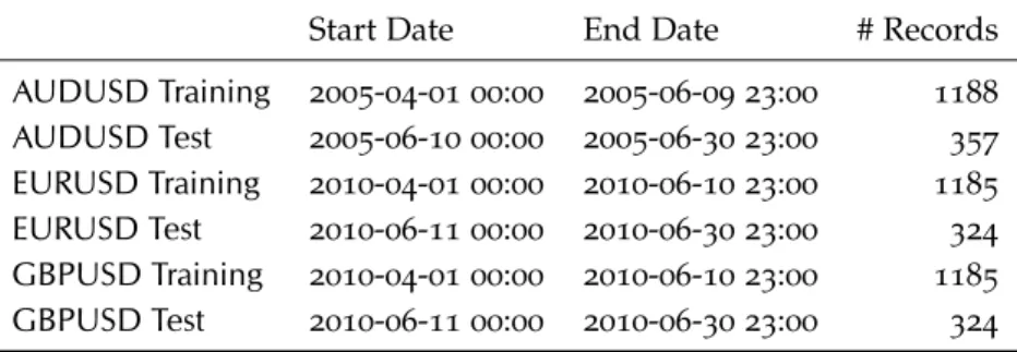
by taking the sum of the signal qualities over the three test data sets, signal strategies that are robust to a wide variety of market conditions have an advantage. The data sets with their respective time intervals and sizes are shown in Table1.

Start Date End Date # Records

AUDUSD Training 2005-04-01 00:00 2005-06-09 23:00 1188 AUDUSD Test 2005-06-10 00:00 2005-06-30 23:00 357 EURUSD Training 2010-04-01 00:00 2010-06-10 23:00 1185 EURUSD Test 2010-06-11 00:00 2010-06-30 23:00 324 GBPUSD Training 2010-04-01 00:00 2010-06-10 23:00 1185 GBPUSD Test 2010-06-11 00:00 2010-06-30 23:00 324

Table1: The training and test data sets with their respective time intervals and sizes used in the competition.

EURUSDandGBPUSDdata are given

for the same time intervals to enable trading strategies to exploit possible correlations.

Tr a d i n gcosts as defined in Section2are given in Table2. These

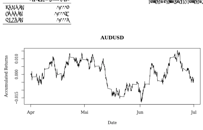
costs, given in counter currency units, apply each time a trade is exited (see Section2). Figure3shows a plot of the accumulated FX

return time seriesAUDUSD, to give an idea of the data. Note the individual returns have been accumulated in this plot. All data sets are made available inCSVformat.

Trading Cost (USD)

AUDUSD 0.0002

EURUSD 0.00015

GBPUSD 0.0003

Table2: Trading cost (given in counter currency units) for each currency pair.

−0.015 0.000 0.010

AUDUSD

Apr Mai Jun Jul

Figure3: The accumulated FX return data setAUDUSD. Shown are both training and test data ranges.

3

Rules and Ranking

The challenge was organized in two rounds: In the first round, participants submitted their score as defined in Section2.1. These

scores are based on the three test data sets given in Section2.2.

They also submitted their executable trading strategy generator. Submissions where ranked by score. In the second and final round, the ten best submissions where be ranked by their scores computed on training and test data sets collected after the submission date, as shown in Table3.

Start Date End Date # Records

Training 2011-04-01 00:00 2011-06-09 23:00 1155

Test 2011-06-10 00:00 2011-06-29 23:00 322

Table3: The training and test data set time intervals and sizes used in the second and final round of the competition. All currency pairs (AUDUSD,EURUSD, andGBPUSD

where sampled in the same time interval and had the same number of records.

A submission’s overall runtime for training per currency pair must not exceed4hours on a modern compute server. The compute

servers used in the final round where equipped with Intel Xeon E5540CPUs (2.53GHz) and4GB RAM.

Implementations of the objective function in both Java and R, ac-companying tools for result analysis, example trading signals, and the training and test data sets will be kept available for download at

Th ewinner of theGECCO 2011Industrial Challenge is the

partici-pant with the highest score in the second round.

4

Results

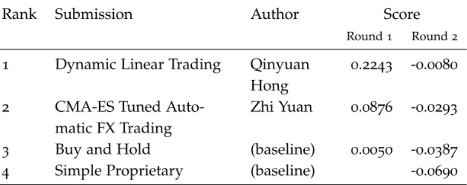
The organizers of theGECCO 2011Industrial Challenge received multiple submissions in the first round. Two submissions gen-erated reproducible results of high enough quality to qualify for the second round. Table4shows the final scores and ranking of

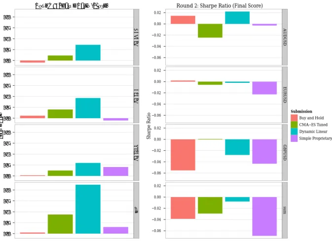
the submissions. These results are also summarized graphically, for both competition rounds,in Figure4. Table5shows the profit

and loss generated by the submissions. To put these results into perspective, a baseline buy and hold and a simple proprietary strat-egy provided by Quaesta Capital GmbH (Simple Proprietary) are shown as baselines.

Rank Submission Author Score

Round1 Round2

1 Dynamic Linear Trading Qinyuan

Hong

0.2243 -0.0080 2 CMA-ES Tuned

Auto-matic FX Trading

Zhi Yuan 0.0876 -0.0293 3 Buy and Hold (baseline) 0.0050 -0.0387 4 Simple Proprietary (baseline) -0.0690

Table4_{: Sharpe ratios (scores) of}

GECCO 2011Industrial Challenge submissions compared with baseline strategies.

Th ebuy and hold baseline strategy is realized by a trading strategy

that generates a constantLongsignal. In this strategy, the portfolio returns directly follow the base currency returns. Trading costs are minimized, as no signal changes occur. Simple Proprietary is a typical trend following strategy used as a building block of the much larger strategy portfolio of Quaesta Capital GmbH. The behavior of this strategy should be similar to other simple strategies available in commercial trading systems.

Rank Submission Author PnL

Round1 Round2

1 Dynamic Linear Trading Qinyuan

Hong

0.1029 -0.0033 2 CMA-ES Tuned

Auto-matic FX Trading

Zhi Yuan 0.0455 -0.0157 3 Buy and Hold (baseline) 0.0056 -0.0210 4 Simple Proprietary (baseline) -0.0411

Table5: Profit and loss (PnL) of

GECCO 2011Industrial Challenge submissions compared with baseline strategies.

Th ewinning submission, "Dynamic Linear Trading" by Qinyuan

fol-lowing strategy incorporating time series embedding preprocess-ing, prediction based on generalized linear models, and algorithm parameter tuning based on grid search. The submission ranked second, "CMA-ES Tuned Automatic FX Trading" by Zhi Yuan of Université Libre de Bruxelles, evolved trading strategies based on three standard technical indicators5

via the well-known Covariance 5

Moving Average (MA), Relative Strength Index (RSI), and Bollinger Bands (BB)

Matrix Adaptation Evolutionary Strategy (CMA-ES).

Round 1: Sharpe Ratio (Score)

Sharpe Ratio 0.00 0.05 0.10 0.15 0.20 0.00 0.05 0.10 0.15 0.20 0.00 0.05 0.10 0.15 0.20 0.00 0.05 0.10 0.15 0.20 AUDUSD EURUSD GBPUSD sum Submission

Buy and Hold CMA−ES Tuned Dynamic Linear Simple Proprietary

Round 2: Sharpe Ratio (Final Score)

Sharpe Ratio −0.06 −0.04 −0.02 0.00 0.02 −0.06 −0.04 −0.02 0.00 0.02 −0.06 −0.04 −0.02 0.00 0.02 −0.06 −0.04 −0.02 0.00 0.02 AUDUSD EURUSD GBPUSD sum Submission Buy and Hold CMA−ES Tuned Dynamic Linear Simple Proprietary

Figure4_{: Summary of the Sharpe} ra-tios (scores) of the submitted strategies in relation with the Buy and Hold and Simple Proprietary baselines. Results of the first round are shown on the left, results of the second round on the right. The ranking is based on the sum of the second round scores.

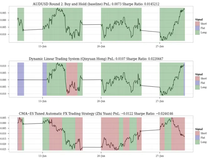
Figure5shows the trading behavior of the submitted trading

strategies, as well as the behavior of the baselines, on theAUDUSD

test data set of the second round. Both submissions outperformed the baseline strategies by a significant margin on the test data sets of both competition rounds.

5

Conclusions and Outlook

An important goal of theGECCO 2011Industrial Challenge was to shed light on the question whether it is possible to generate profitable algorithmic trading strategies based on FX return data alone. While both submissions that qualified for the second round significantly outperformed the baseline strategies in both rounds, the results also indicate that the profitability of trading strategies

AUDUSD Round 2: Buy and Hold (baseline) PnL: 0.0073 Sharpe Ratio: 0.0145212 Cumulative Return −0.010 −0.005 0.000 0.005

13−Jun 20−Jun 27−Jun

Signal

Short Flat Long

Dynamic Linear Trading System (Qinyuan Hong) PnL: 0.0107 Sharpe Ratio: 0.0220447

Cumulative Return−0.010 −0.005 0.000 0.005 0.010

13−Jun 20−Jun 27−Jun

Signal

Short Flat Long

CMA−ES Tuned Automatic FX Trading Strategy (Zhi Yuan) PnL: −0.0122 Sharpe Ratio: −0.0244146

Cumulative Return−0.025 −0.020 −0.015 −0.010 −0.005 0.000 0.005

13−Jun 20−Jun 27−Jun

Signal

Short Flat Long

Figure5_{: Trading signals and return} generated by submitted strategies compared with the Buy and Hold baseline strategy, on theAUDUSDdata set of the second (i.e. final) round.

Shortsignals are shown in red,Flat

signals in blue, andLongsignals in green. Returns are shown in units of counter currency.

is highly dependent on the given market environment. Successful strategies must adapt as the market environment changes. Quaesta Capital GmbH is very interested in the results obtained.

The Industrial Challenge will continue atGECCO 2012, again featuring a highly relevant industry problem provided by an indus-try partner. More information and the official call for participation will soon be available athttp://gociop.deand through the official

GECCO 2012channels.

5

.

1

Organizing Committee

• Thomas Bartz-Beielstein, Cologne University of Applied Sciences • Oliver Flasch, Cologne University of Applied Sciences

• Wolfgang Kantschik, DIP Dortmund Intelligence Project GmbH • Christian von Strachwitz, Quaesta Capital GmbH

• Wolfgang Konen, Cologne University of Applied Sciences • Pier Luca Lanzi, Politecnico di Milano

References

M.P. Austin, G. Bates, M.A.H. Dempster, V. Leemans, and S.N. Williams. Adaptive systems for foreign exchange trading. Quanti-tative Finance,4(4):37–45, August2004. ISSN1469-7688.

S. Bhattacharyya, O.V. Pictet, and G. Zumbach. Knowledge-intensive genetic discovery in foreign exchange markets. IEEE Transactions on Evolutionary Computation,6(2):169–181, April2002.

P.J. Brockwell and R.A. Davis. Introduction to Time Series and

Fore-casting. Springer, New York NY,2002. ISBN0387953515.

M.A.H. Dempster and Y.S. Romahi. Intraday FX trading: An evolutionary reinforcement learning approach. In H. Yin, N.M. Allinson, R.T. Freeman, J.A. Keane, and S.J. Hubbard, editors,

Proceedings of Third International Conference on Intelligent Data

En-gineering and Automated Learning - IDEAL2002, volume2412of

Lecture Notes in Computer Science, pages347–358, Manchester,2002.

Springer. ISBN3540440259.

J.D. Hamilton. Time Series Analysis. Princeton University Press,1

edition, January1994. ISBN0691042896.

T. Weithers. Foreign Exchange: A Practical Guide to the FX Markets. Wiley Finance. John Wiley & Sons, Inc.,2006. ISBN9780470043363.

G. Wilson and W. Banzhaf. Soft memory for stock market analysis using linear and developmental genetic programming. InGenetic

and Evolutionary Computation Conference GECCO ’09(Proceedings),

pages1633–1640, New York, NY, USA,2009. ACM. ISBN978-1 -60558-325-9.

G. Wilson and W. Banzhaf. Interday foreign exchange trading using linear genetic programming. InGenetic and Evolutionary

Computation Conference GECCO ’10(Proceedings), pages1139–1146,