Financial
Institutions
Center
Statistical Analysis of a Telephone Call
Center: A Queueing-Science Perspective
by Lawrence Brown Noah Gans Avishai Mandelbaum Anat Sakov Haipeng Shen Sergey Zeltyn Linda Zhao 03-12
The Wharton Financial Institutions Center
The Wharton Financial Institutions Center provides a multi-disciplinary research approach to
the problems and opportunities facing the financial services industry in its search for
competitive excellence. The Center's research focuses on the issues related to managing risk
at the firm level as well as ways to improve productivity and performance.
The Center fosters the development of a community of faculty, visiting scholars and Ph.D.
candidates whose research interests complement and support the mission of the Center. The
Center works closely with industry executives and practitioners to ensure that its research is
informed by the operating realities and competitive demands facing industry participants as
they pursue competitive excellence.
Copies of the working papers summarized here are available from the Center. If you would
like to learn more about the Center or become a member of our research community, please
let us know of your interest.
Franklin Allen
Richard J. Herring
Co-Director
Co-Director
The Working Paper Series is made possible by a generous
grant from the Alfred P. Sloan Foundation
Statistical Analysis of a Telephone Call Center:
A Queueing-Science Perspective
∗Lawrence Brown, Noah Gans, Avishai Mandelbaum, Anat Sakov, Haipeng Shen, Sergey Zeltyn and Linda Zhao
November 9, 2002
Corresponding author: Lawrence D. Brown
Department of Statistics, The Wharton School, University of Pennsylvania, Philadelphia, PA 19104-6340
Email: [email protected], Phone: (215)898-4753, Fax: (215)898-1280
∗Lawrence Brown is Professor, Department of Statistics, The Wharton School, University of Pennsylvania,
(email: [email protected]). Noah Gans is Assistant Professor, Department of Operations and Informa-tion Management, The Wharton School, University of Pennsylvania, (email: [email protected]). Avishai Mandelbaum is Professor, Faculty of Industrial Engineering and Management, Technion, Haifa, Israel, (email: [email protected]). Anat Sakov is post-doctoral fellow, Faculty of Industrial Engineering and Manage-ment, Technion, Haifa, Israel, (email: [email protected]). Haipeng Shen is Ph.D. Candidate, Department of Statistics, The Wharton School, University of Pennsylvania, (email: [email protected]). Sergey Zel-tyn is Ph.D. Candidate, Faculty of Industrial Engineering and Management, Technion, Haifa, Israel, (email: [email protected]). Linda Zhao is Associate Professor, Department of Statistics, The Wharton School, University of Pennsylvania, (email: [email protected]). This work was supported by the ISF (Israeli Science Founda-tion) Grants 388/99 and 126/02, the Wharton Financial Institutions Center, the NSF and the Technion funds for the promotion of research and sponsored research.
Abstract
A call center is a service network in which agents provide telephone-based services. Customers that seek these services are delayed in tele-queues.
This paper summarizes an analysis of a unique record of call center operations. The data comprise a complete operational history of a small banking call center, call by call, over a full year. Tak-ing the perspective of queueTak-ing theory, we decompose the service process into three fundamental components: arrivals, customer abandonment behavior and service durations. Each component involves different basic mathematical structures and requires a different style of statistical analysis. Some of the key empirical results are sketched, along with descriptions of the varied techniques required.
Several statistical techniques are developed for analysis of the basic components. One of these is a test that a point process is a Poisson process. Another involves estimation of the mean function in a nonparametric regression with lognormal errors. A new graphical technique is introduced for nonparametric hazard rate estimation with censored data. Models are developed and implemented for forecasting of Poisson arrival rates.
We then survey how the characteristics deduced from the statistical analyses form the building blocks for theoretically interesting and practically useful mathematical models for call center oper-ations.
Key Words: call centers, queueing theory, lognormal distribution, inhomogeneous Poisson process, censored data, human patience, prediction of Poisson rates, Khintchine-Pollaczek formula, service times, arrival rate, abandonment rate, multiserver queues.
Contents
1 INTRODUCTION 1
1.1 Highlights of results . . . 2
1.2 Structure of the paper . . . 4
2 QUEUEING MODELS OF CALL CENTERS 4 3 THE CALL CENTER OF BANK ANONYMOUS 5 4 THE ARRIVAL PROCESS 7 4.1 Arrivals are inhomogeneous Poisson . . . 9
4.2 The Poisson arrival-rates are not easily “predictable” . . . 13
5 SERVICE TIME 15 5.1 Very short service times . . . 16
5.2 On service times and queueing theory . . . 17
5.3 Service times are lognormal . . . 18
5.4 Regression of log service times on time-of-day . . . 19
5.4.1 Estimation ofµ(·) . . . 19
5.4.2 Estimation ofσ2(·) . . . 20
5.4.3 Estimation ofν(·) . . . 20
5.4.4 Application and model diagnostics . . . 21
6 QUEUEING TIME: WAITING TIME FOR SERVICE OR ABANDONING 23 6.1 Waiting times are exponentially distributed . . . 23
6.2 Survival curves for virtual waiting time and patience . . . 24
6.3 Hazard rates . . . 27
6.5 Dependence, or the violation of classical assumptions of survival analysis . . . 31
7 PREDICTION OF THE LOAD 32 7.1 Definition of load . . . 32
7.2 Independence of Λ(t) and ν(t) . . . 33
7.3 Coefficient of Variation for the prediction of L(t) . . . 34
7.4 Prediction of Λ(t) . . . 35
7.5 Diagnostics for the model for Λ(t) . . . 38
7.6 Prediction ofν(t) . . . 38
7.7 Confidence intervals forL(t) . . . 40
8 SOME APPLICATIONS OF QUEUEING SCIENCE 41 8.1 Validating Classical Queueing Theory . . . 42
8.2 Fitting the M/M/N+M model (Erlang-A) . . . 46
8.2.1 The Erlang-A Model . . . 47
8.2.2 Approximations . . . 49
8.2.3 Use and Limits of the Erlang-A Model . . . 50
1
INTRODUCTION
Telephone call centersallow groups of agents to serve customers remotely, via the telephone. They have become a primary contact point between customers and their service providers and, as such, play an increasingly significant role in more developed economies. For example, it is estimated that call centers handle more than 70% of all business interactions and that they employ more than 3.5 million people, or 2.5% of the workforce, in the U.S. (Uchitelle, 2002; Call Center Statistics, 2002). While call centers are technology-intensive operations, often 70% or more of their operating costs are devoted to human resources, and to minimize costs their managers carefully track and seek to maximize agent utilization. Well-run call centers adhere to a sharply-defined balance between agent efficiency and service quality, and to do so, they use queueing-theoretic models. Inputs to these mathematical models are statistics concerning system primitives, such as the number of agents working, the rate at which calls arrive, the time required for a customer to be served, and the
length of time customers are willing to wait on hold before they hang up the phone andabandon
the queue. Outputs are performance measures, such as the distribution of time that customers wait “on hold” and the fraction of customers that abandon the queue before being served. In practice, the number of agents working becomes a control parameter which can be increased or decreased to attain the desired efficiency-quality tradeoff.
Often, estimates of two or more moments of the primitives are needed to calibrate queueing models, and in many cases, the models make distributional assumptions concerning the primitives. In theory, the data required to validate and properly tune these models should be readily available, since computers track and control the minutest details of every call’s progress through the system. It is thus surprising that operational data, collected at an appropriate level of detail, has been scarcely available. The data that are typically collected and used in the call-center industry are
simpleaveragesthat are calculated for the calls that arrive within fixed intervals of time, often 15
or 30 minutes. There is thus a lack of documented, comprehensive, empirical research on call-center performance that employs more detailed data.
The immediate goal of our study is to fill this gap. In this paper, we summarize a comprehensive analysis of operational data from a bank call center. The data span all twelve months of 1999 and are collected at the level of individual calls. Our data source consists of over 1,200,000 calls that arrived to the center over the year. Of these, about 750,000 calls terminated in an interactive voice response unit (IVR or VRU), a type of answering machine that allows customers serve themselves. The remaining 450,000 callers asked to be served by an agent, and we have a record of the event-history of each of these calls.
1.1 Highlights of results
1. The arrival times of calls requesting service by an agent are extremely well modelled as an inhomogeneous Poisson process. This is not a surprise. The process has a smoothly varying
rate function,λ, that depends, in part, on the date, time of day, type and priority of the call.
(See Section 4.1.)
2. The function λis a hidden (or latent) rate function that it is not observed. That is, λis not
functionally determined by date, time, and call-type information. Because of this feature, we develop models to predict statistically the number of arrivals as a function of only these repetitive features. The methods also allows us to construct confidence bounds related to these predictions. See also Brown, Mandelbaum, Sakov, Shen, Zeltyn and Zhao (2002), where these models are more fully developed. (See Sections 4.2 and 7.4.)
3. The times required to serve customers of various types have lognormal distributions. This is quite different from the exponential distribution customarily assumed for such times, a finding that has potentially important implications for the queueing theory used to model the process. (See Section 5.3.)
4. The lognormal nature of service times has also led us to develop new methods for nonparamet-ric estimation of regression models involving lognormal errors, as well as for the generation of confidence and prediction intervals. (The mean time, as opposed to the median or the mean of the log-time, is of central interest to queueing theory, and this necessitates more precise tools for statistical inference about the mean.) Some of these new methods are reported here; others will be included in Shen (2002). (See Section 5.4.)
5. A surprising feature is the presence of a disproportionate number of extremely short service times, under 5 seconds. (Presumably these are mainly due to agents who prematurely discon-nect from the customer without offering any real service.) This reflects a behavioral feature of service agents that needs to be taken into account (and discouraged by various means) in engineering a queueing system. This feature also needs to be suitably accommodated in order to correctly estimate the parameters and features of the service-time distribution. (See Section 5.1.)
6. A joint feature of the arrivals and service times is that they are noticeably positively corre-lated as a function of time-of-day (and given customer types and priorities). Thus, during the busiest times of day (10am-12pm and 2pm-4pm) the service times are also, on average, longest. We are not sure what the explanation is for this and have developed several alter-nate hypotheses. Section 7 reports an examination of the data to see whether one of these can be identified as the primary cause. Determination of the cause could noticeably affect calculations of the so-called “offered load” that is central to queueing-theoretic calculation of system performance. (See Sections 4.1, 5.4 and 7.2.)
7. The hazard rate of customer patience is estimated using a competing-risks model for censored data. The very large size of our data set makes this an unusual situation for such an analysis, and it enables us to develop new nonparametric methods and graphical techniques. One notably finding is a marked short-run increase in the propensity of customers to abandon the queue at times shortly after they receive a message that asks them to be patient. We also examine two different patience indices that measure the relationship between customer patience and waiting time, and investigate the observed relationship between them. (See Sections 6.3 and 6.4.)
8. We examine the validity of a queueing-theoretic rule that relates the average waiting time in queue to the probability of abandonment. This “ratio” rule is derived in Baccelli and Hebuterne (1981) and Zohar, Mandelbaum and Shimkin (2002) and holds for models with exponentially distributed patience. We find that the rule seems to hold with reasonable preci-sion for our data, even though customers’ patience distribution is noticeably non-exponential. We are currently searching for a theoretical explanation of this empirical observation. (See Section 8.1.)
9. It is also possible to check the applicability of a multiple-server generalization of the classical Khintchine-Pollaczek formula from queueing theory (Iglehart and Whitt, 1970; Whitt, 2002). The data show that this formula does not provide a reasonable model for the call center under study, a result that is not surprising in that the formula ignores customer abandonment behavior. Conversely, alternatives that explicitly account for abandonment, such as Baccelli and Hebuterne (1981) and Garnett, Mandelbaum and Reiman (2002), perform noticeably better. (See Section 8.)
10. It is of interest to note that relatively simple queueing models can turn out to be surprisingly robust. For example, when carefully tuned, the so-called M/M/N+M model can be made to fit performance measures reasonably accurately, even though characteristics of the theoretical primitives clearly do not conform with the empirical ones. (See Section 8.2.)
Our study also constitutes a prototype that paves the way for larger-scale studies of call centers. Such a study is now being conducted under the auspices of the Wharton Financial Institutions Center.
This paper is part of a larger effort to use both theoretical and empirical tools to better characterize call center operations and performance. Mandelbaum, Sakov and Zeltyn (2000) presents a com-prehensive descriptive analysis of our call-by-call database. Zohar et al. (2002) considers customer patience and abandonment behavior. Gans, Koole and Mandelbaum (2002) reviews queueing and related capacity-planning models of call centers, and it describes additional sources of call-center data (marketing, surveys, benchmarking). Mandelbaum (2001) is a bibliography of more than 200 academic papers related to call-centers.
1.2 Structure of the paper
The paper is structured as follows. In Section 2, we provide theoretical background on queueing models of call centers. Next, in Section 3, we describe the call center under study and its database. Each of Sections 4 to 6 is dedicated to the statistical analysis of one of the stochastic primitives of the queueing system: Section 4 addresses call arrivals; Section 5, service durations; and Section 6, tele-queueing and customer patience. Section 6 also analyzes customer waiting times, a performance measure that, interestingly, is deeply intertwined with the abandonment primitive.
A synthesis of the primitive building blocks is typically needed for operational understanding. To this end, Section 7 discusses prediction of the arriving “workload”, which is essential in practice for setting suitable service staffing levels.
Once each of the primitives has been analyzed, one can also attempt to use existing queueing theory, or modifications thereof, to describe certain features of the holistic behavior of the system. In Section 8 we conclude with analyses of this type. We validate some classical theoretical results from queueing theory and refute others.
2
QUEUEING MODELS OF CALL CENTERS
Call centers agents provide tele-services. As they speak with customers over the phone, they
interact with a computer terminal, inputting and retrieving information related to customers and their requests. Customers, who are only virtually present, are either being served or are waiting
in what we call atele-queue, a phantom queue which they share, invisible to each other and to the
agents who serve them. Customers wait in this queue until one of two things happen: an agent is
allocated to serve them (through supporting software), or they becomeimpatientandabandonthe
tele-queue.
Queueing theory was conceived by A.K. Erlang (Erlang, 1911; Erlang, 1917) at the beginning of the 20th century and has flourished since to become one of the central research themes of Operations Research (For example, see Wolff 1989, Buzacott and Shanthikumar 1993 and Whitt 2002). In a queueing model of a call center, the customers are callers, the servers are telephone agents or communications equipment, and queues are populated by callers that await service.
The queueing model that is simplest and most widely used in call centers is the so-called M/M/N
system, sometimes called the Erlang-C model.1 Given arrival rateλ, average service durationµ−1
1The first M in “M/M/N” comes from Poisson arrivals, equivalently exponentially distributed, or Markovian,
interarrival times. The second M, from Markovian (exponential) service times. The N denotes the number of servers working in parallel.
and N servers working in parallel, the Erlang-C formula, C(λ, µ, N), describes, theoretically, the long-run fraction of time that all N servers will be simultaneously busy, or (via PASTA, see Wolff 1989) the fraction of customers who are delayed in queue before being served. In turn, it allows for calculation of the theoretical distribution of the length of time an arriving customer will have to wait in queue before being served.
The Erlang-C model is quite restrictive, however. It assumes, among other things, a steady-state environment in which arrivals conform to a Poisson process, service durations are exponentially dis-tributed, and customers and servers are statistically identical and act independently of each other. It does not acknowledge, among other things, customer abandonment behavior, time-dependent parameters, or customer heterogeneity. We refer the reader to Sze (1984), Harris, Hoffman and Saunders (1987), Garnett and Mandelbaum (1999), Garnett et al. (2002) and Zohar et al. (2002) for an elaboration of the Erlang-C’s shortcomings. An essential task of queueing theorists is to develop models that account for the most important of these effects.
Queueing science seeks to determine which of these effects is most important. For example, Garnett et al. (2002) develops both exact and approximate expressions for “Erlang-A” systems, which explicitly model customer patience (time to abandonment) as exponentially distributed. Data analysis of the arrival process, service times, and customer patience can confirm or refute whether system primitives conform to the Erlang-C and A models’ assumptions. Empirical analysis of waiting times can help us to judge how well the two models predict customer delays – whether or not their underlying assumptions are met.
3
THE CALL CENTER OF BANK ANONYMOUS
The source of our data is a small call center of one of Israel’s banks. (The small size has proved very convenient, in many respects, for a pioneering field study.) The center provides several types of services: information for current and prospective customers, transactions for checking and savings accounts, stock trading, and technical support for users of the bank’s internet site. On weekdays (Sunday through Thursday in Israel) the center is open from 7am to midnight; it closes at 2pm on Friday, for the weekend, and reopens around 8pm on Saturday. During working hours, at most 13 regular agents, 5 internet agents, and one shift supervisor may be working.
A simplified description of the path each call follows through the center is as follows. A customer calls one of several telephone numbers associated with the call center, the number depending on the type of service sought. Except for rare busy signals, the customer is then connected to a VRU and identifies herself. While using the VRU, the customer receives recorded information, general and customized (e.g. an account balance). It is also possible for the customer to perform some self-service transactions here, and 65% of the bank’s customers actually complete their service via
the VRU. The other 35% indicate the need to speak with an agent. If there is an agent free who is capable of performing the desired service, the customer and the agent are matched to start service immediately. Otherwise the customer joins the tele-queue.
Customers in the tele-queue are nominally served on a first-come first-served (FCFS) basis, and cus-tomers’ places in queue are distinguished by the time at which they arrive to the queue. In practice, the call center operates a priority system with two priorities - high and low - and moves high-priority customers up in queue by subtracting 1.5 minutes from their actual arrival times. Mandelbaum et al. (2000) compares differences between the behaviors of the two groups of customers.
While waiting, each customer periodically receives information on her progress in the queue. More specifically, she is told the amount of time that the first in queue has been waiting, as well as her approximate location in the queue. The announcement is replayed every 60 seconds or so, with music, news, or commercials intertwined.
Figure 1 provides a schematic summary of the event history (process flow) of calls through the system. In the figure, the numbers next to arrows represent approximate numbers of calls each month that arrived to the VRU, queue, abandoned, were served. From the figure, we see that in each of the 12 months of 1999, roughly 100,000-120,000 calls arrived to the system with 65,000-85,000 terminating in the VRU. The remaining 30,000-40,000 calls per month involved callers who exited the VRU indicating a desire to speak to an agent. The percentages within the ovals show that about 80% of those requesting service were, in fact served, and about 20% abandoned before being served. The focus of our study is the set of 30,000-40,000 calls each month that crossed Figure 1’s dashed line and queued or were immediately served.
Figure 1: Event history of calls (units are calls per month)
VRU / IVR Queue Service
End of Service ~17% of those Abandon requesting service End of Service ~83% of those requesting service 100-120K 22K 16K 29K 6K 65-85K 13K
Each call that crosses the dashed line can be thought of as passing through up to three stages,
each of which generates distinct data. The first is thearrival stage, which is triggered by the call’s
exit from the VRU and generates a record of an arrival time. If no appropriate server is available,
then the call enters thequeueingstage. Three pieces of data are recorded for each call that queues:
queue, by being served or abandoning. The last stage is service, and data that are recorded are the starting and ending times of the service. Note that calls that are served immediately skip the queueing stage, and calls that abandon never enter the service stage.
In addition to these time stamps, each call record in our database includes a categorical description of the type of service requested. The main call types are Regular (PS in the database), Stock Transaction (NE), New Customer (NW), and Internet Assistance (IN). (Two other types of call – Service in English (PE) and Outgoing Call (TT) – exist. Together, they accounted for less than 2% of the calls in the database, and they have been omitted from the analysis reported here.) Our database includes calls for each month of 1999, and over the year there were two operational changes that are important to note. First, from January through July, all calls were served by the same group of agents, but beginning in August, internet (IN) customers were served by a separate pool of agents. Thus, from August through December the center can be considered to be two separate service systems, one for IN customers and another for all other types. Second, as will be noted in Section 5, one aspect of the service-time data changed at the end of October. In several instances this paper’s analyses are based on only the November and December data. In other instances we have used data from August through December. Given the changes noted above, this ensures consistency throughout the manuscript. November and December were also convenient because they contained no Israeli holidays. In these analyses, we also restrict the data to include only regular weekdays – Sunday through Thursday, 7am to midnight – since these are the hours of full operation of the center. We have performed similar analyses for other parts of the data, and in most respects the November–December results do not differ noticeably from those based on data from other months of the year.
4
THE ARRIVAL PROCESS
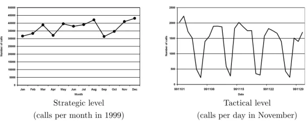
Buffa, Cosgrove and Luce (1976) describes four levels of representation of a call center that differ according to their time scales. Information about the system at these levels is required to support the complex task of efficiently staffing a center. The two top levels are the monthly (“strategic”) level and daily (“tactical”) level. Figure 2 shows plots of the arrival of calls at these two levels. The strategic level is presented in an annual plot with month being the time unit. The decrease in calls in April and September is due to many holidays in these months. Strategic information is required to determine how many agents are needed in all, perhaps by season, and it affects hiring and training schedules.
The tactical level is presented here in a monthly plot with day as the unit. The valleys occur during weekends when the center is only open for a few hours per day. Daily information is used to determine work assignments: given the total number of employees available, more or fewer agents
Figure 2: Arrival process plots (monthly and daily level)
-DQ )HE 0DU $SU 0D\ -XQ -XO $XJ 6HS 2FW 1RY 'HF 0RQWK ,90
Strategic level Tactical level
(calls per month in 1999) (calls per day in November)
are required to work each day, depending (in part) on the total number of calls to be answered. It should be clear that information at both of these levels is important for proper operation of the center. We will concentrate our analysis on the finer levels, however: hourly (“operational”); and real time (“stochastic”). Queueing models operate at these levels, and they are also the levels that present the most interesting statistical challenges.
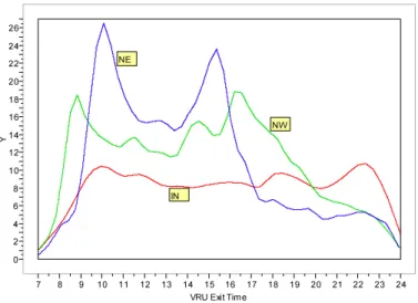
Figures 3 and 4 show, as a function of time of day, the average rate per hour at which calls come out of the VRU. These are composite plots for weekday calls in November and December. The plots show calls according to the major call types. The volume of Regular (PS) calls is much greater than that of the other 3 types; hence those calls are shown on a separate plot. These plots are kernel estimates using normal kernels. (The kernels have sd = 0.15 for the first plot and sd = 0.25 for the others. The bandwidths were visually chosen to preserve most of the regular variability evident in a histogram with 10 minute bin-widths.) For a more precise study of these arrival rates, including confidence and prediction intervals see Section 7 and also Brown et al. (2002) and Brown, Zhang and Zhao (2001).
Note the bimodal pattern of Regular call-arrival times in Figure 3. It is especially interesting that Internet service calls (IN) do not show a similar bimodal pattern and, in fact, have a peak in volume after 10pm. (We speculate that this peak can be partially explained by the fact that internet customers are sensitive to telephone rates, which significantly decrease in Israel after 10pm, and they also tend to be late-night types of people.)
Figure 3: Arrivals (to queue or service); Regular Calls/Hr; Weekdays Nov.–Dec. 0 20 40 60 80 100 120 C al ls /H r ( R eg ) 7 8 9 10 11 12 13 14 15 16 17 18 19 20 21 22 23 24 VRU Exit Time
Figure 4: Arrivals (to queue or service); IN, NW, and NE Calls/Hr; Weekdays Nov.–Dec.
0 2 4 6 8 10 12 14 16 18 20 22 24 26 Y 7 8 9 10 11 12 13 14 15 16 17 18 19 20 21 22 23 24 VRU Exit Time
NE
NW
IN
4.1 Arrivals are inhomogeneous Poisson
Classical theoretical models posit that arrivals form a Poisson process. It is well known that such a process results from the following behavior: there exist many potential, statistically identical callers to the call center; there is a very small yet non-negligible probability for each of them calling at any given minute, say, so that the average number of calls arriving within a minute is moderate; and callers decide whether or not to call independently of each other.
Common call-center practice assumes that the arrival process is Poisson with a rate that remains constant for blocks of time, often individual half-hours or hours. A call center will then fit a separate
queueing model for each block of time, and estimated performance measures may shift abruptly from one interval to the next.
A more natural model for capturing both stochastic and operational levels of detail is a time inhomogeneous Poisson process. Such a process is the result of time-varying probabilities that individual customers call, and it is completely characterized by its arrival-rate function. To be useful for constructing a (time inhomogeneous) queueing model, this arrival-rate function should vary smoothly and not too rapidly throughout the day. Smooth variation of this sort is familiar in both theory and practice in a wide variety of contexts, and seems reasonable here.
We now construct a test of the null hypothesis that arrivals of given types of calls form an inhomo-geneous Poisson process, with the arrival rate varying slowly. This test procedure does not assume that the arrival rates (of a given type) depend only on the time-of-day and are otherwise the same from day to day. It also does not require the use of additional covariates to (attempt to) estimate the arrival rate for given date and time-of-day.
The first step in construction of the test involves breaking up the interval of a day into relatively
short blocks of time. For convenience we used blocks of equal time-length, L, resulting in a total
of I blocks, though this equality assumption could be relaxed. For the Regular (PS) data we used
L= 6 minutes. For the other types we usedL= 60 minutes, since these types involved much lower
arrival rates. One can then consider the arrivals within a subset of blocks – for example, blocks at
the same time on various days or successive blocks on a given day. Let Tij denote the j-th ordered
arrival time in the i-th block, i = 1, . . . , I. Thus Ti1 ≤ . . . ≤TiJ(i), where J(i) denotes the total
number of arrivals in thei-th block. Then define Ti0= 0 and
Rij = (J(i) + 1−j) −log L−Tij L−Ti,j−1 , j= 1, ..., J(i).
Under the null hypothesis that the arrival rate is constant within each given time interval, the
{Rij}will be independent standard exponential variables as we now discuss.
Let Uij denote the j-th (unordered) arrival time in the i-th block. Then the assumed constant
Poisson arrival rate within this block implies that, conditionally onJ(i), the unordered arrival times
are independent and uniformly distributed, i.e. Uij i.i.d.∼ U(0, L). Note thatTij =Ui(j). It follows
that LL−−TTij
i,j−1 are independent Beta(J(i) + 1−j,1) variables. (See, for example, Problem 6.14.33(iii)
in Lehmann 1986.) A standard change of variables then yields the exponentiality of theRij. (One
may alternatively base the test on the variables Rij∗ = j
−logTTij
i,j+1
where j = 1, . . . , J(i) and
Ti,J(i)+1 = L. Under the null hypothesis these will also be independent standard exponential
variables.)
The null hypothesis does not involve an assumption that the arrival rates of different intervals are equal or have any other pre-specified relationship. Any customary test for the exponential
distri-bution can be applied to test the null hypothesis. For convenience we use the familiar Kolmogorov-Smirnov test, even though this may not have the greatest possible power against the alternatives of most interest.
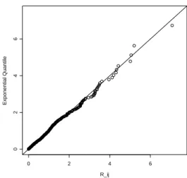
Figures 5 and 6 display the results of two applications of this test. Figure 5 is an exponential
quantile plot for the {Rij}computed from arrival times of the Regular (PS) calls arriving between
11:12am and 11:18am on all weekdays in November and December. Figure 6 is a similar plot from arrival of IN calls throughout Monday, November 23; from 7am to midnight. This was a typical midweek day in our data set.
Figure 5: Exponential (λ=1) Quantile plot for {Rij} from Regular calls 11:12am – 11:18am; Nov.
and Dec. weekdays
R_ij
Exponential Quantile
0 2 4 6
024
6
For both of the examples, pictured in Figures 5 and 6, the null hypothesis is not rejected, and we conclude that their data are consistent with the assumption of an inhomogeneous Poisson process for the arrival of calls. The respective Kolmogorov-Smirnov statistics have values K = 0.0316 (P-value = 0.2 with n = 420) and K = 0.0423 (P-(P-value = 0.2 with n = 172). These results are typical of those we have obtained from various selections of blocks of the various types of calls. Thus, overall there is no evidence in this data set to reject a null hypothesis that the arrival of calls from the VRU is an inhomogeneous Poisson process.
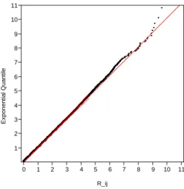
As a further demonstration that the arrival times follow an inhomogeneous Poisson process, we applied this method to the 48,963 Regular (PS) calls in November and December in blocks of 6 minutes for calls exiting the VRU on weekdays between 7am and 12pm. In view of the very large sample size we should expect the null hypothesis to be rejected, since the arrival rate is not exactly constant over 6 minute intervals, and also since the data are recorded in discrete units (of seconds) rather than being exactly continuous, as required by the ideal assumptions in the null hypothesis.
Figure 6: Exponential (λ=1) Quantile plot for {Rij}from Internet calls; Nov. 23 R_ij Exponential Quantile 0 1 2 3 4 5 6 01234 56
With this in mind, we view the fidelity of the exponential quantile plot in Figure 7 to a straight line as remarkable evidence that there is no discernible deviation of any practical importance from the assumption that the arrival data follow the law of an inhomogeneous Poisson process. (Two
outlying values of Rij have been omitted in Figure 7. They correspond to two 6-minute intervals
in which the telephone switching system apparently malfunctioned.)
Figure 7: Exponential Quantile plot of{Rij}for all PS calls, weekdays in Nov.–Dec. (Two outliers
omitted.) Ex ponential Q uantile 1 2 3 4 5 6 7 8 9 10 11 0 1 2 3 4 5 6 7 8 9 10 11 R_ij
We note that in this section, as well as in the following section, many tests are performed on the same data. For example, we test for the Poisson property over different blocks of time, different
days, different types of service etc. This introduces the problem of multiple testing: when many null hypotheses are rejected, a question should be asked if the rejections are real. One way to account for the problem is to use the FDR procedure (Benjamini and Hochberg, 1995). We do not use the procedure here since we are mainly illustrating what can be done with the data, rather than using them to make operational inferences. However, it is critical to use FDR or other procedures when making operational inferences.
4.2 The Poisson arrival-rates are not easily “predictable”
The inhomogeneous Poisson process described above provides a stochastic regularity that can some-times be exploited. However, this regularity is most valuable if the arrival rates are known, or can be predicted on the basis of observable covariates. The current section examines the hypothesis that the Poisson rates can be written as a function of the available covariates: call type, time-of-day and day-of-the-week. If this were the case, then these covariates could be used to provide valid stochastic predictions for the numbers of arrivals. But, as we now show, this is not the case. The null hypothesis to be tested is, therefore, that the Poisson arrival rate is a (possibly unknown)
function λtype(d, t), where type ∈ {P S, N E, N W, IN} may be any one of the types of customers,
d ∈ {Sunday, . . . ,Thursday} is the day of the week, and t ∈ [7,24] is the time of day. For this
discussion, let ∆ be a specified calendar date (e.g. November 7th), and let Ntype,∆ denote the
observed number of calls requesting service of the given type on the specified date. Then, under
the null hypothesis, the Ntype,∆ are independent Poisson variables with respective parameters
E[Ntype,∆] =
24
7 λtype(d(∆), t)dt , (1)
whered(∆) denotes the day-of-week corresponding to the given date.
Under the null hypothesis, each set of samples for a given type and day-of-week,{Ntype,∆|d(∆) =
d}, should consist of independent draws from a common Poisson random variable. If so, then one
would expect the sample variance to be approximately the same as the sample mean. For example, see Agresti (1990) and Jongbloed and Koole (2001) for possible tests.
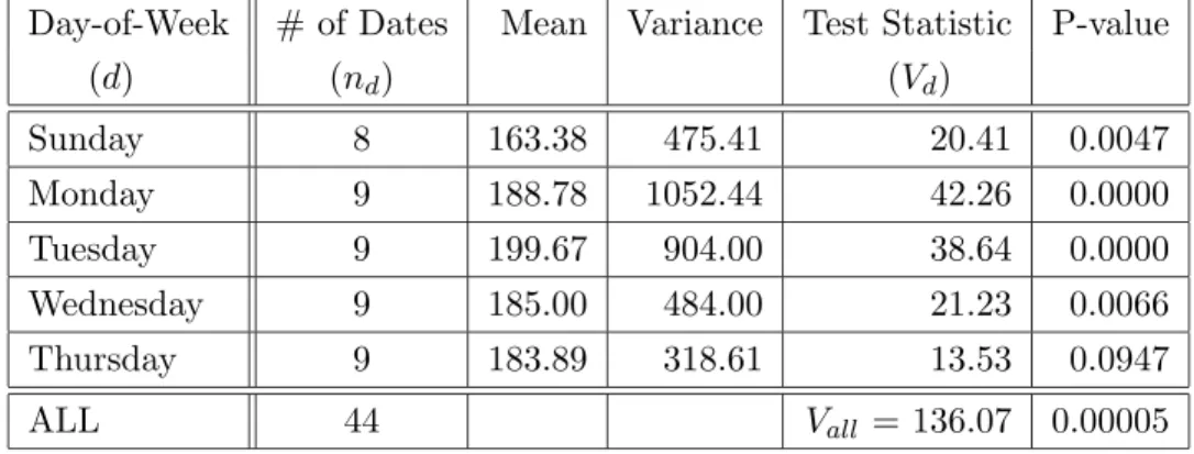
Table 1 gives some summary statistics for the observed values of {NN E,∆|d(∆) =d} for weekdays
in November and December. Note that there were 8 Sundays and 9 each of Monday through
Thursday during this period. A glance at the data suggests that the {NN E,∆|d(∆) = d} are
not samples from Poisson distributions. For example, the sample mean for Sunday is 163.38, and the sample variance is 475.41. This observation can be validated by a formal test procedure, as described in the following paragraphs.
Table 1: Summary statistics for observed values of NN E,∆, weekdays in Nov. and Dec.
Day-of-Week # of Dates Mean Variance Test Statistic P-value
(d) (nd) (Vd) Sunday 8 163.38 475.41 20.41 0.0047 Monday 9 188.78 1052.44 42.26 0.0000 Tuesday 9 199.67 904.00 38.64 0.0000 Wednesday 9 185.00 484.00 21.23 0.0066 Thursday 9 183.89 318.61 13.53 0.0947 ALL 44 Vall = 136.07 0.00005
variables. This is the test employed below. The background for this test is Anscombe’s variance stabilizing transformation for the Poisson distribution (Anscombe, 1948).
To apply this test to the variables{NN E,∆|d(∆) =d}, calculate the test statistic
Vd = 4 × {∆|d(∆)=d} NN E,∆+ 3/8 − 1 nd {∆|d(∆)=d} NN E,∆+ 3/8 2 ,
where nd denotes the number of dates satisfying d(∆) = d. Under the null hypothesis that the
{NN E,∆|d(∆) =d} are independent identically distributed Poisson variables, the statistic Vd has
very nearly a Chi-squared distribution with (nd−1) degrees of freedom. The null hypothesis should
be rejected for large values of Vd. Table 1 gives the values of Vd for each value of d, along with
the P-values for the respective tests. Note that for these five separate tests the null hypothesis is
decisively rejected for all but the valued= Thursday.
It is also possible to use the {Vd} to construct a test of the pooled hypothesis that the NN E,∆
are independent Poisson variables with parameters that depend only on d(∆). This test uses
Vall=
Vd. Under the null hypothesis this will have (very nearly) a Chi squared distribution with
(nd−1) degrees of freedom, and the null hypothesis should be rejected for large values of Vall.
The last row of Table 1 includes the value of Vall, and the P-value is less than or equal to 0.00005.
The qualitative pattern observed in Table 1 is fairly typical of those observed for various types of calls, over various periods of time. For example, a similar set of tests for type NW for November
and December yields one non-significant P-value (P = 0.2 ford(∆) = Sunday), and the remaining
P-values are vanishingly small. A similar test for type PS (Regular) yields all vanishingly small P-values.
The tests above can also be used on time spans other than full days. For example, we have con-structed similar tests for PS calls between 7am and 8am on weekdays in November and December.
(A rationale for such an investigation would be a theory that early morning calls – before 8am – arrive in a more predictable fashion than those later in the day.) All of the test statistics are
extremely highly significant: for example the value ofVall is 143 on 39 degrees of freedom. Again,
the P-value is less than or equal to 0.00005.
In summary, we saw in Section 4.1 that, for a given customer type, arrivals are inhomogeneous Poisson, with rates that depend on time of day as well as on other possible covariates. In Section 4.2 an attempt was made to characterize the exact form of this dependence, but ultimately the hypothesis was rejected that the Poisson rate was a function only of these covariates. For the operation of the call center it is desirable to have predictions, along with confidence bands, for this rate. We return to this issue in Section 7.
5
SERVICE TIME
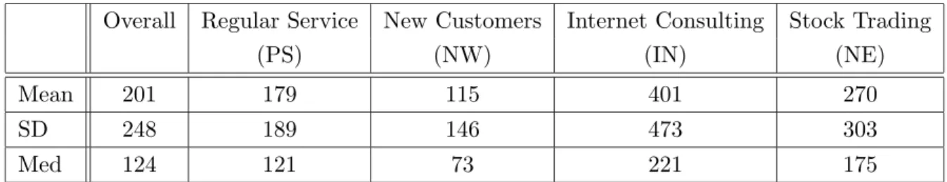
The last phase in a successful visit to the call center is typically the service itself. Table 2 summarizes the mean, SD and median service times for the four types of service of main interest. The very few calls with service time larger than an hour were not considered (i.e. we treat them as outliers). Adding these calls has little effect on the numbers.
Table 2: Service time by type of service, truncated at 1 hour, Nov.–Dec.
Overall Regular Service New Customers Internet Consulting Stock Trading
(PS) (NW) (IN) (NE)
Mean 201 179 115 401 270
SD 248 189 146 473 303
Med 124 121 73 221 175
Internet consulting calls have the longest service times, and trading services are next in duration. New customers have the shortest service time (which is consistent with the nature of these calls). An important implication is that the workload that Internet consultation imposes on the system is more than its share in terms of percent of calls. This is an operationally important observation to which we will return in Section 7.
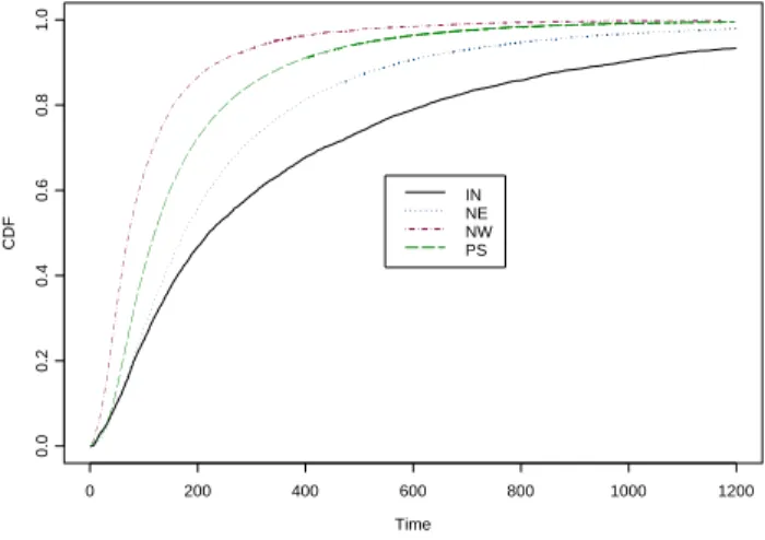
Figure 8 plots the cumulative distribution functions of service times by type. Note the clear stochas-tic ordering among the types, which strengthens the previously-discovered inequalities among mean service times.
Figure 8: Service times cumulative distribution functions, by types, Nov.–Dec. Time CDF 0 200 400 600 800 1000 1200 0.0 0.2 0.4 0.6 0.8 1.0 IN NE NW PS
5.1 Very short service times
Figure 9 shows histograms of the combined service times for all types of service for January through October and for November–December. These plots resemble those for Regular Service calls alone, since the clear majority of calls are for regular service. Looking closely at the histograms, we see that, in the first 10 months of the year, the percent of calls with service shorter than 10 seconds was larger than the percent at the end of the year (7% vs. 2%).
Figure 9: Distribution of service time
Time Jan-Oct 0 100 200 300 400 500 600 700 800 900 0 2 4 6 8 7.2 % Mean = 185 SD = 238 Time Nov-Dec 0 100 200 300 400 500 600 700 800 900 0 1 2 3 4 5 6 7 8 5.4 % Mean = 200 SD = 249
Service times shorter than 10 seconds are questionable. And, indeed, the manager of the call
center discovered that short service times were primarily caused by agents that simply hung-upon
uncommon; it is often due to distorted incentive schemes, especially those that over-emphasize short average talk-time, or equivalently, the total number of calls handled by an agent). The problem was identified and steps were taken to correct it in October of 1999, after a large number of customers had complained about being disconnected. For this reason, in the later analysis we focus on data from November and December. Suitable analyses can be constructed for the entire year through the use of a mixture model or (somewhat less satisfactorily) by deleting from the service-time analysis all calls with service times under 10 seconds.
5.2 On service times and queueing theory
Most applications of queueing theory to call centers assume exponentially distributed service times as their default. The main reason is the lack of empirical evidence to the contrary, which leads one to favor convenience. Indeed, models with exponential service times are amenable to analysis, especially when combined with the assumption that arrival processes “are” Poisson processes (a rather natural one for call centers, see Section 4.1). The prevalent M/M/N (Erlang-C) model is an example.
In more general queueing formulae, the service time often affects performance measures through its
squared-coefficient-of-variation C2 =σ2/E2, E being the average service time, andσ its standard
deviation. For example, a useful approximation for the average waiting time in an M/G/N model (Markovian arrivals, Generally distributed service times, N servers), is given by Whitt (1993):
E[Wait for M/G/N]≈E[Wait for M/M/N] × (1 +C
2)
2 .
Thus, average wait with general service times is multiplied by a factor of (1 +C2)/2 relative to the
wait under exponential service times. For example, if service times are, in fact, exponential then
the factor is 1, as should be; deterministic service timeshalvethe average wait of exponential; and
finally, based on Table 2, our empirical (1 +C2)/2 = 1.26.
In fact, in the approximation above and many of its “relatives”, service times manifest themselves only through their means and standard deviations. Consequently, for practical purposes, if means and standard deviations are close to each other, then one assumes that system performance will be close to that with exponential service times.
However, for large call centers with high levels of agent utilization, this assumption may not hold:
simulation studies indicate that theentiredistribution of service time may become very significant
(for example, see Mandelbaum and Schwartz 2002). While ours is a small call center with moderate utilization levels, its service-time distributions are, nevertheless, likely to be similar to those of larger, more heavily utilized systems. Thus, it is worthwhile investigating the distribution of its service times.
5.3 Service times are lognormal
Looking at Figure 9, we see that the distribution of service times is clearly not exponential, as assumed by standard queueing theory. In fact, after separating the calls with very short service
times, our analysis reveals a remarkable fit to the lognormaldistribution.
The left panel of Figure 10 shows the histogram of log(service time) for November and December, in which the short service phenomenon was absent or minimal. We also superimpose the best fitted normal density as provided by Brown and Hwang (1993). The right panel shows the lognormal Q-Q plot of service time, which does an amazingly good imitation of a straight line. Both plots suggest that the distribution of Service Time is very nearly lognormal. We only provide the graphs to qualitatively support our claim of lognormality. The reason is that, given the large sample size we have, the Kolmogorov-Smirnov test (or any other goodness-of-fit test) will always reject the null hypothesis of lognormality due to a small deviation from the lognormal distribution.
Figure 10: Histogram, QQ Plot of Log(Service Time) (Nov.–Dec.)
0 2 4 6 8 0.0 0.1 0.2 0.3 0.4 Log(Service Time) Proportion Log-normal Service time 0 1000 2000 3000 0 1000 2000 3000
After excluding short service times, the strong resemblance to a lognormal distribution also holds for all other months. It also holds for various types of callers even though the parameters depend on the type of call. This means that, in this case, a mixture of log-normals is log-normal empirically, even though mathematically this cannot hold. The same phenomenon occurs in Section 6.1, when discussing the exponential distribution. We refer the reader to Mandelbaum et al. (2000) where the phenomenon is discussed in the context of the exponential distribution.
Lognormality of processing times has been occasionally recognized by researchers in telecommuni-cations and psychology. Bolotin (1994) shows empirical results which suggest that the distribution of the logarithm of call duration is normal for individual telephone customers and a mixture of nor-mals for “subscriber-line” groups. Ulrich and Miller (1993) and Breukelen (1995) provide theoretical arguments for the lognormality of reaction times using models from mathematical psychology.
Man-delbaum and Schwartz (2002) use simulations to study the effect of lognormally distributed service times on queueing delays.
In our data, lognormality appears to also hold quite well at lower levels: for all types and priorities of customers, for individual servers, for different days of the week, and also when conditioning on time of day, as in Section 5.4. Brown and Shen (2002) gives a more detailed analysis of service times.
5.4 Regression of log service times on time-of-day
The important implication of the excellent fit to a lognormal distribution is that we can apply standard techniques to regress log(service time) on various covariates, such as time-of-day. For example, to model the mean service time across time-of-day, we can first model the mean and variance of the log(service time) across time-of-day and then transform the result back to the service-time scale. (Shen (2002) contains a detailed analysis of service service-times against other covariates, such as the identities of individual agents (servers), as well as references to other literature involving lognormal variates.)
LetS be a lognormally distributed random variable with meanν and varianceτ2, thenY = log(S)
will be a normal random variable with some mean µand varianceσ2. It is well known that
ν=eµ+12σ2. (2)
We use (2) as a basis for our proposed methodology. Suppose we wish to estimate ν =E(S) and
construct an associated confidence interval. If we can derive estimates forµandσ2, then ˆν=eµˆ+σˆ22
will be a natural estimate for ν according to (2). Furthermore, in order to provide a confidence
interval forν, we need to derive confidence intervals for µand σ2, or more precisely, forµ+σ2/2.
For our call center data, letS be the service time of a call andT be the corresponding time-of-day
that the call begins service. Let{Si, Ti}ni=1be a random sample of sizenfrom the joint distribution
of{S, T}and sorted according toTi. Then Yi = log(Si) will be the Log(Service Time) of the calls,
and these are (approximately) normally distributed, conditional on Ti. We can fit a regression
model ofYi on Ti as
Yi =µ(Ti) +σ(Ti)i, (3)
wherei|Ti are i.i.d. N(0,1).
5.4.1 Estimation of µ(·)
If we assume thatµ(·) has a continuous third derivative, then we can use local quadratic regression
µ(t0), then an approximate 100(1−α)% confidence interval for µ(t0) is
ˆ
µ(t0)±zα/2seµ(t0), (4)
where seµ(t0) is the standard error of the estimate of the mean at t0 from the local quadratic fit.
5.4.2 Estimation of σ2(·)
Our estimation of the variance functionσ2(·) is a two-step procedure. At the first step, we regroup
the observations{Ti, Yi}in=1 into consecutive non-overlapping pairs{T2i−1, Y2i−1;T2i, Y2i}i=1n/2. The
variance atT2i,σ2(T2i), is estimated by a squared pseudo-residual,D2i, of the form (Y2i−1−Y2i)2/2,
a so-called difference-based estimate. The difference-based estimator we use here is a simple one that suffices for our purposes. In particular, our method yields suitable confidence intervals for
the estimation ofσ2. More efficient estimators might slightly improve our results. There are many
other difference-based estimators in the literature. See M¨uller and Stadtm¨uller (1987), Hall, Kay
and Titterington (1990), Dette, Munk and Wagner (1998) and Levins (2002) for more discussions of difference-based estimators.
During the second step, we treat {T2i, D2i}i=1n/2 as our observed data points and apply local
quadratic regression to obtain ˆσ2(t0). Part of our justification is that, under our model (3), the
{D2i}’s are (conditionally) independent given the{T2i}’s. Similar to (4), a 100(1−α)% confidence
interval forσ2(t0) is approximately
ˆ
σ2(t0)±zα/2seσ2(t0).
Note that we usezα/2 as the cutoff value when deriving the above confidence interval, rather than
a quantile from a Chi-square distribution. Given our large data set the degree of freedom is large, and a Chi-square distribution can be approximated well by a normal distribution.
5.4.3 Estimation of ν(·)
We now use ˆµ(t0) and ˆσ2(t0) to estimate ν(t0), as eµˆ(t0)+ˆσ2(t0)/2. Given the estimation methods
used forµ(t0) andσ2(t0), ˆµ(t0) and ˆσ2(t0) are asymptotically independent, which gives us
se(ˆµ(t0) + ˆσ2(t0)/2)≈ seµ(t0)2+ seσ2(t0)2/4.
When the sample size is large, we can assume that µ(·) +σ2(·)/2 has an approximately normal
distribution. Then the corresponding 100(1−α)% confidence interval for ν(t0) is
exp
(ˆµ(t0) + ˆσ2(t0)/2)±zα/2 seµ(t0)2+ seσ2(t0)2/4
.
5.4.4 Application and model diagnostics
In the following analysis, we apply the above procedure to the weekday calls of November and De-cember. The results for two interesting service types are shown in Figures 11 and 12, below. There
are 42,613 Regular Service (PS) calls and 5,066 Internet Consulting (IN) calls. To produce the
figures, we use the tricube function as the kernel and nearest-neighbor type bandwidths. The band-widths are subjectively chosen to generate interesting curves that are nearly free of (apparently) extraneous wiggles.
Figure 11 shows the mean service time for PS calls as a function of time-of-day, with 95% confidence bands. Note the prominent bimodal pattern of mean service time across the day for PS calls. The accompanying confidence band shows that the changing pattern is highly significant. Average service times are longest around 10:00am and 3:00pm. The changing pattern of the overall average (across all types of calls) will be similar, because about 70% of the calls are Regular Service calls.
Also notice that the pattern nicely resembles that for arrival rates of PS calls. (See Figure 3
in Section 4.) Call center managers should take this phenomenon into account when making
operational decisions. We will come back to this issue and explore possible explanations when we analyze system workload in Section 7.
Figure 11: Mean Service Time (PS) versus Time-of-day (95% CI)
Time of Day
Mean Service Time
10 15 20 100 120 140 160 180 200 220 240 7 8 9 10 11 12 13 14 15 16 17 18 19 20 21 22 23 24
Figure 12 plots an analogous confidence band for IN calls. One interesting observation is that IN calls do not show a similar bimodal pattern. We do see some fluctuations during the day, but they are only mildly significant, given the wide confidence band. Also notice that the entire confidence band for IN calls lies above that of PS calls. This reflects the same stochastic dominance that was observed in Figure 8.
Figure 12: Mean Service Time (IN) versus Time-of-day (95% CI)
Time of Day
Mean Service Time
10 15 20 300 350 400 450 500 7 8 9 10 11 12 13 14 15 16 17 18 19 20 21 22 23 24
We close this section with some diagnostics of our model, looking at residuals from the regression of log(service time) on time-of-day for PS calls. Figure 13’s histogram and normal quantile plot of residuals show that the residuals are fairly normal, and they provide additional validation of the lognormality of the service times.
Figure 13: Histogram, QQ Plot of The Residuals from Modeling Mean Log(Service Time) on Time-of-day (PS) -4 -2 0 2 4 0.0 0.1 0.2 0.3 0.4 Residuals Proportion
Quantiles of Standard Normal
Residuals -4 -2 0 2 4 -4 -2 0 2 4
6
QUEUEING TIME: WAITING TIME FOR SERVICE OR
ABAN-DONING
In Sections 4 and 5 we characterized two primitives of queueing models: the arrival process and service times. In each case we were able to directly observe and analyze the primitive under investigation.
Ideally, we would next address the last system primitive, customer patience and abandonment behavior, before considering system outputs, such as waiting time. Abandonment behavior and waiting times are deeply intertwined, however. By definition, all customers who abandon the
tele-queue have waited. Furthermore, the times at which customers who are served would have
abandoned, had they not been served, are not observed. Thus, the characterization of patience and time to abandonment is based on censored data.
We make three important outcome-based distinctions. The first is the difference between queueing time and waiting time. We use the convention that the latter does not account for zero-waits. This measure is more relevant for managers, especially when considered jointly with the fraction of customers that did wait. A second, more fundamental, distinction is between the waiting times of customers who were served and of those who abandoned. A third distinction is between the
time that a customer needs to wait before reaching an agent versus the time that a customer is
willing to wait before abandoning the system. The former is referred to as virtual waiting time, since it amounts to the time that a (virtual) customer, equipped with infinite patience, would have
waited until being served. We refer to the latter aspatience. Both measures are obviously of great
importance, but neither is directly observable, and hence both must be estimated.
6.1 Waiting times are exponentially distributed
A well known queueing-theoretic result is that, in heavily loaded systems (in which essentially all customers wait, so that queueing time equals waiting time), queueing time should be exponentially distributed. See Kingman (1962) for an early result and Whitt (2002) for a recent text. Although our system is not very heavily loaded, we find that the empirical waiting time distribution conforms to the theoretical prediction.
Table 3 summarizes the mean, SD and median waiting time for all calls, as well as for calls stratified by outcome (A – Abandoned; S – Served) and by type of service. The waiting-time data have some observations that we consider to be outliers: for example, those with queueing time larger than 5 hours. Therefore, we have truncated the waiting time at 15 minutes. This captures about 99% of the data.
Table 3: Waiting time, truncated at 15 minutes (A – Abandoned; S – Served) Overall PS NE NW IN A S A S A S A S A S Mean 98 78 105 62 96 99 114 88 136 140 159 SD 105 90 108 69 98 113 112 94 131 148 159 Med 62 51 67 43 62 55 78 58 92 86 103
exponential distribution, and the figure’s right panel compares the waiting times to exponential
quantiles, using a Q-Q plot. (Thep-value for the Kolmogorov-Smirnov test for exponentiality is 0
however. This is not surprising in view of the large sample size of about 48,000.)
Figure 14: Distribution of waiting time (1999)
Time 0 30 60 90 120 150 180 210 240 270 300 29.1 % 20 % 13.4 % 8.8 % 6.9 % 5.4 % 3.9 % 3.1 % 2.3 % 1.7 % Mean = 98 SD = 105 Waiting time Exp quantiles 0 200 400 600 0 200 400 600
In fact, when restricted to customers reaching an agent, the histogram of waiting time resembles even more strongly an exponential distribution. Similarly, each of the means in Table 3 is close to the corresponding standard deviation, both for all calls and for those that reach an agent. This suggests (and was verified by QQ-plots) an exponential distribution also for each stratum, where a similar explanation holds: calls of type PS are about 70% of the calls. We also observe this exponentiality when looking at the waiting time stratified by months (Table 4).
6.2 Survival curves for virtual waiting time and patience
Both times to abandonment and times to service are censored data, and we apply survival
anal-ysis to help us estimate them. Denote by R the “patience” or “time willing to wait”, by V the
Table 4: Waiting time, truncated at 15 minutes
Jan Feb Mar Apr May Jun Jul Aug Sep Oct Nov Dec
Mean 68 76 119 109 96 85 105 114 84 73 101 111
SD 67 78 126 108 101 89 105 119 89 83 109 116
Med 46 50 75 72 62 55 69 72 54 45 63 71
W = min{R, V}, as well as the indicator 1{R<V} for observing R or V. To estimate the
distribu-tion ofR, one considers all calls that reached an agent as censored observations, and vice versa for
estimating the distribution ofV. We make the assumption that (as random variables)RandV are
independent given the covariates relevant to the individual customer. Under this assumption, the
distributions ofRand V (given the covariates) can be estimated using the standard Kaplan-Meier
product-limit estimator. (See Section 6.5 for some cautionary remarks.)
In Figure 15, we plot the Kaplan-Meier estimates of the survival functions of R (time willing to
wait), V (virtual waiting time) and W = min{V, R}. A clear stochastic ordering emerges among
the three distributions. Moreover, the same ordering arises at all months and across different types
of service. The reason for the survival function ofW being the lowest is obvious. In contrast, the
stochastic ordering betweenV andR is interesting and informative. It indicates that customers are
willing to wait (R) more than they need to wait (V), which suggests that our customers population
consists of patient customers. Here we have implicitly, and only intuitively, defined the notion of a
patient customer(to the best of our knowledge systematic research on this subject is lacking).
In Figure 16, we consider the survival functions of R for different types of service. Again, a clear
stochastic ordering emerges. For example, we learn that customers performing stock trading (type ‘NE’) are willing to wait more then customers calling for regular services (type ‘PS’). One might intuitively expect stock-trading customers to be less tolerant of delay. At the same time, their need for service, and their trust of the system to provide it, might be higher. Thus, a possible explanation for the ordering shown in Figure 16 is that type NE needs the service more urgently, and we are led to distinguish between tolerance for waiting and loyalty/persistency (which we do not pursue further).
Table 5 reports the means and standard deviations of the conventional Kaplan-Meier estimates for
the distributions of V andR. The table is based on all weekday calls in November and December
that waited in queue. We use a procedure that is conventional in several standard software packages. When the Kaplan-Meier estimate of the survival distribution of the event is defective (does not reach 0) this conventional estimator places all remaining survival probability at the largest event time.
Figure 15: Survival curves (Nov.–Dec.) Time Survival 0 200 400 600 800 1000 0.0 0.2 0.4 0.6 0.8 1.0 W R V
Figure 16: Survival curves for time willing to wait (Nov.–Dec.)
Time Survival 0 500 1000 1500 2000 2500 3000 0.0 0.2 0.4 0.6 0.8 1.0 IN NE NW PS
anomalies. In spite of the fact that one expects the true distributions to be skewed to the right, the estimated distributions are severely truncated. This is especially true for types PS and NE because they are more heavily censored. See Figure 16. A result of this is that the estimated means for PS and NE calls are much smaller than the estimated medians, while the opposite relation holds for
Table 5: Means, SDs and medians forV and R (Nov.–Dec.)
Time willing to wait (R) Time needs to wait (V)
Mean SD Median Mean SD Median
All Combined 803 905 457 142 161 96
PS 642 446 1048 118 114 83
NE 806 471 1225 144 141 103
NW 535 885 169 227 251 193
IN 550 591 302 274 319 155
NW and IN calls. Also the estimated mean for the overall distribution (mean = 803) is much larger than that for its largest component, PS (mean = 642) and is approximately equal to the largest of the component means. We suspect that, as a consequence of this heavy censoring, the estimates
for the mean of R are heavily biased (too small) and should be handled with care. Again this is
especially true for types PS and NE in this table.
6.3 Hazard rates
Hazard rates are informative for understanding time-varying behavior. For example, local peaks in the hazard rates of the time willing to wait manifest a systematically increased tendency to abandon, while constant hazard rates indicate that the tendency to abandon remains the same, regardless of the past (memoryless). Palm (1953) was the first to describe impatience in terms of a hazard rate. He postulated that the hazard rate of the time-willing-to-wait is proportional to a customer’s irritation due to waiting (thus defining, implicitly, the notion of irritation). Aalen and Gjessing (2001) advocate dynamic interpretation of the hazard rate, but warn against the possibility that the population hazard rate need not represent individual ones.
For this reason we have found it useful to construct nonparametric estimates of the hazard rate. It is feasible to do so because of the large sample size of our data (about 48,000). Figures 17 and 18
show such plots for R andV, respectively.
The procedure we use to calculate and plot the figures is as follows. For each interval of length δ,
the estimate of the hazard rate is calculated as
[ # of events during (t, t+δ] ]
[ # at risk at t] × δ .
For smaller time values, t, the numbers at risk and event rates are large, and we letδ = 1 second.
For larger times, when fewer are at risk, larger δ’s are used. Specifically, the larger intervals are
the hazard rate for each interval is plotted at the interval’s median.
The curves superimposed on the plotted points are fitted using nonparametric regression. In prac-tice we used LOCFIT (Loader, 1999), though other techniques, such as kernel procedures or smooth-ing splines, would yield similar fits. In particular, we have experimented with HEFT (Kooperberg, Stone and Truong, 1995), as can be seen in Mandelbaum et al. (2000). The smoothing bandwidth was chosen manually to provide a reasonably smooth estimate which, nevertheless, provided a sat-isfying visual fit to the data. We experimented with fitting techniques that varied the bandwidth to take into account the increased variance and decreased density of the estimates with increasing time. However, with our data these techniques had little effect and so are not used here.
Figure 17 plots the hazard rates of the time willing to wait for regular (PS) calls. Note that it shows two main peaks. The first occurs after only a few seconds. When customers enter the queue, a “Please wait” message, as described in Section 3, is played for the first time. At this point some customers who do not wish to wait probably realize they are in queue and hang up. The second
peak occurs at about t= 60, about the time the system plays the message again. Apparently, the
message increases customers’ likelihood of hanging up for a brief time thereafter, an effect that may be contrary to the message’s intended purpose (or, maybe not!).
Figure 17: Hazard rate for the time willing to wait for PS calls (Nov.–Dec.)
Time Hazard Rate 0 200 400 600 800 0.0 0.002 0.004 0.006
In Figure 18, the hazard rate for the virtual waiting times is estimated forallcalls (the picture for
each type is very similar). The overall plot reveals rather constant behavior beyond 100 seconds, which suggests exponentiality of the tail.