Evolutionary Algorithms: Application to
Cardiac SPECT Diagnosis
António Gaspar-Cunha
IPC/I3N – Institute of Polymers and Composites, University of Minho, Campus de Azurém, Guimarães, Portugal (e-mail: [email protected]).
Abstract
An optimization methodology based on the use of Multi-Objective Evolutionary Algorithms (MOEA) in order to deal with problems of feature selection in data mining was proposed. For that purpose a Support Vector Machines (SVM) fier was adopted. The aim being to select the best features and optimize the classi-fier parameters simultaneously while minimizing the number of features necessary and maximize the accuracy of the classifier and/or minimize the errors obtained. The validity of the methodology proposed was tested in a problem of cardiac Sin-gle Proton Emission Computed Tomography (SPECT). The results obtained allow one to conclude that MOEA is an efficient feature selection approach and the best results were obtained when the accuracy, the errors and the classifiers parameters are optimized simultaneously.
1. Introduction
Feature selection is of crucial importance when dealing with problems with high amount of data. This importance can be due to various reasons: i) the processing of all features available can be computational infeasible; ii) the existence of high number of variables for small number of available data points can invalidate the resolution of the problem; iii) an high number of features can be redundant or ir-relevant for the classification problem under study. Therefore, taking into account the large number of variables usually present, and the frequent correlation between these variables, the existence of a feature selection method able to reduce the number of features considered for analysis is of essential importance [1].
Multi Objective Evolutionary Algorithms (MOEA) is a valid and efficient method to deal with this problem. Recently, some works using this approach have been proposed. A framework for SVM based on multi-objective optimization with
the aim of minimizes the risk of the classifier and the model capacity (or accuracy) was proposed by Bi [2]. An identical approach was followed by Igel [3], but now the objective concerning the minimization of the risk was replaced by the minimi-zation of the complexity of the model (i.e., the number of features). Oliveira et al. in [4] used an hierarchical MOEA operating at two levels: performing a feature lection to generate a set of classifiers (based on artificial neural networks) and se-lecting the best set of classifiers. Hamdani et al. in [5] optimized simultaneously the number of features and the global error obtained by a neural network classifier using the NSGA-II algorithm [6]. Both errors of type I (false positive) and type II (false negative) were taking into account individually through the application of a MOEA by Alfaro-Cid et al. [7]. MOEA were also applied in unsupervised learn-ing. Handl and Knowles studied the problem of feature selection by formulating them as a multi-objective optimization problem [8].
The main ideas of a previous work proposed by the author were take into ac-count [9]. It consisted in using a MOEA to accomplish simultaneously two objec-tives: the minimization of the number of features used and the maximization of the accuracy of the classifier used [9]. This is an important issue since parameter tun-ing is not an easy task [10]. In this work these ideas were extended to deal with the issue of selecting the best accuracy measures [11-13]. Thus, different accuracy measures, such as maximization of the Fmeasure and the minimization of errors (type I and type II) will be tested. Also, an analysis based on ROC curves will be carried out [13]. Simultaneously, the parameters required by the classifier will be optimized. The motivation for doing this work is the development of a methodol-ogy able to deal with bigger problems like gene expression data. However, before applying the methodology to difficult problems the methodology must be tested in small and controllable problems.
This text is organized as follows. The MOEA used will be presented and de-scribed in detail in section 2. In section 3 the classification methods employed and the main accuracy measures employed will be presented and described. The meth-odology proposed will be applied to a case study and the results will be presented and discussed in section 4. Finally, the conclusion will be drawn in section 5.
2. Multi-Objective Evolutionary Algorithms
Due to the complexity in dealing with multiple conflicting objectives problems, MOEAs have been recognized in the last two decades as good methods to explore and find an approximation to the Pareto-optimal front. This is due to the difficulty of traditional exact methods to solve this type of problems and by their capacity to explore and combine various solutions to find the Pareto front in a single run. The Pareto front is constituted by the non-dominated solutions, i.e., the solutions that are not better neither worst than the others. Thus, a MOEA must be able to ac-complish simultaneously two objectives, a homogeneous distribution of the
popu-lation along the Pareto frontier in the objective domain and an improvement of the solutions along successive generations [6, 14]. The Reduced Pareto Set Genetic Algorithm with elitism (RPSGAe) is adopted here [14, 15]. This algorithm is based on the use of a clustering technique to reduce the number of solutions on the efficient frontier, which enabled simultaneously the distribution of the solutions along the entire Pareto front and the choice of the best solutions for reproduction. Thus, both the exploration and exploitation of the search space are simultaneously taking into account. Detailed information about this algorithm can be found else-where [14, 15].
3. Classification Methods
The methodology proposed here consists in using a MOEA to determine the best compromise between the two and/or the three conflicting objectives. For that pur-pose Support Vector Machines (SVM) will be used to evaluate (or classify) the trial solutions proposed by the MOEA during the successive generations. Support Vector Machines (SVMs) are a set of supervised learning methods based on the use of a kernel, which can be applied to classification and regression. In the SVM a hyper-plane or set of hyper-planes is (are) constructed in a high-dimensional space. In this case, a good separation is achieved by the hyper-plane that has the largest distance to the nearest training data points of any class. Thus, the generali-zation error of the classifier is lower when this margin is larger. SVMs can be seen an extension to nonlinear models of the generalized portrait algorithm developed by Vapnik in [16]. In this work the SVM from LIBSVM was used [17].
The SVM performance depends strongly on the selection of the right kernel, as well the definition of the best kernel parameters [3]. In the present study only the C-SVC method using as kernel the Radial Basis Function (RBF) was tested [17]. Thus, two different SVM parameters are to be selected carefully: the regulariza-tion parameter (C) and the kernel parameter (γ). Another important parameter is the training method. Two different approaches were used for training the SVM, holdout and 10-fold validation. Thus two additional parameters were studied: the Learning Rate (LR) and the Training Fraction (TF). The choice of a performance metric to evaluate the learning methods is nowadays an important issue that must be carefully defined [11-13]. Some recent studies demonstrate that the use of a single measure can introduce an error on the classifier evaluation, since two type of objectives must be accomplished simultaneously, maximization of the classifier accurateness and minimization of the errors obtained [13]. The selection of the best learning algorithm to use and the best performance metric to measure the ef-ficiency of the classifier is nowadays the subject of many studies [11, 13].
The simplest way evaluate a classifier is the use the accuracy given by the ratio between the number instances correctly evaluated and the total number of in-stances, i.e., Accuracy = (TP + TN) /(TP + TN + FP + FN), where, TP are the
posi-tives correctly classified, TN are the negatives correctly classified, FP are the posi-tives incorrectly classified and FN are the negative incorrectly classified. It is also important to know the level of the errors accomplished by the classifier. Two dif-ferent error types can be defined, type I and type II, given respectively by: eI =
FP/(FP + TN) and eII = FN/(FN + TP). Another traditional way to evaluate the in-formation is using the sensitivity or recall (R) and the precision (P) of the classi-fier: R = TP/(TP + FN) and P = TP/(TP + FN). Fmeasure, representing the harmonic mean of R and P, is a global measure often used to evaluate the classifier: Fmeasure = (2.P.R)/(P + R). In order to take into account the problem of simultaneously maximize the classifier accurateness and minimize the errors obtained, ROC curves can be adopted instead [12, 13]. On a ROC graph the False Positive rate (FPrate) is plotted in the X axis and the True Positive rate (TPrate) is plotted on the Y axis. Thus, defining a bi-dimensional Pareto frontier where the aim is to ap-proach the left top corns of this graph [12, 13]. The FPrate is given by the error of type I (eI) and the TPrate is given by the recall (R).
4. Results and Discussion
The MOEA methodology proposed will be used in a diagnostic problem of cardiac Single Proton Emission Computed Tomography (SPECT) images [18]. Each of the patients is classified into two categories: normal and abnormal. The database of 267 SPECT image sets (patients) was processed to extract features that summa-rize the original SPECT images. As a result, 44 continuous feature patterns were created for each patient. The pattern was further processed to obtain 22 binary fea-ture patterns. The aim was finding the minimum number of feafea-tures while maxi-mizing the accuracy and/or the Fmeasure and minimizing the errors. The database was downloaded from the UCI Machine Learning Repository [19].
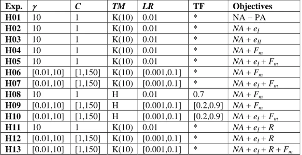
Table 1 shows the different experiments tested. Concerning the definition of the decision variables, two possibilities were considered. Initially, a pure feature selection problem was analyzed. In this case the parameters of the classifier, such as type of training and learning rate, the SVM parameters (C and γ) and the train-ing fraction of holdout validation, were initially set. In a second approach, these parameters were also included as variables to be optimized. The range of variation allowed for these variables is shown on Table 1. The RPSGAe was applied using the following parameters: 100 generations, crossover rate of 0.8, mutation rate of 0.05, internal and external populations with 100 individuals, limits of the cluster-ing algorithm set at 0.2 and the number of ranks (NRanks) at 30. These values re-sulted from a carefully analysis made previously [14, 15]. Due to the stochastic nature of the initial tentative solutions several runs have to be performed (in the present case 10 runs) for each experiment. Thus, a statistical method based on at-tainment functions was applied to compare the final population for all runs [20, 21]. This method attributes to each objective vector a probability that this point is
attaining in one single run [20]. It is not possible to compute the true attainment function, but it can be estimated based upon approximation set samples, i.e., dif-ferent approximations obtained in difdif-ferent runs, which is denoted as Empirical Attainment Function (EAF) [21]. The differences between two algorithms can be visualized by plotting the points in the objective space where the differences be-tween the empirical attainment functions of the two algorithms are significant [22]. Table 1. Experiments. Exp. γ C TM LR TF Objectives H01 10 1 K(10) 0.01 * NA + PA H02 10 1 K(10) 0.01 * NA + eI H03 10 1 K(10) 0.01 * NA + eII H04 10 1 K(10) 0.01 * NA + Fm H05 10 1 K(10) 0.01 * NA + eI + Fm H06 [0.01,10] [1,150] K(10) [0.001,0.1] * NA + Fm H07 [0.01,10] [1,150] K(10) [0.001,0.1] * NA + eI + Fm H08 10 1 H 0.01 0.7 NA + Fm H09 [0.01,10] [1,150] H [0.001,0.1] [0.2,0.9] NA + Fm H10 [0.01,10] [1,150] H [0.001,0.1] [0.2,0.9] NA + eI + Fm H11 10 1 K(10) 0.01 * NA + eI + R H12 [0.01,10] [1,150] K(10) [0.001,0.1] * NA + eI + R H13 [0.01,10] [1,150] K(10) [0.001,0.1] * NA + eI + R + Fm * Not applicable
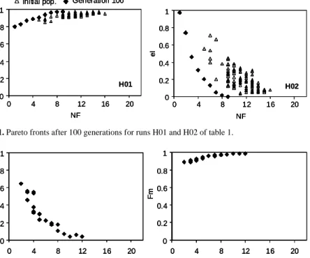
Figure 1 shows the initial population and the Pareto front after 100 generations for the first run of Experiments H01 and H02 (Table 1). Identical results were ob-tained for the remaining runs. As can be observed there is a clear improvement of the solutions proposed during the search process. The algorithm was able to evolve to good values of the Accuracy (graph at the left) using a few features. In fact only six or seven features are needed to reach more than 90% of accuracy. Concerning the experiments were the eI was minimized simultaneously with the number of features (H02) identical improvements can be noticed. More results can
be found at http://www.dep.uminho.pt/agc/agc/Supplementary_Information_Page.html.
The results for the first run of experiment 5 were plotted in Figure 2. In this case a 3-dimensional Pareto front was obtained and some of the points that seem to be dominated in one of the graphs (in each 2D plots) are in reality non-dominated due to the third objective considered in the optimization run. These plots are very similar to those obtained for experiments H01 and H02, but now the solutions resulted from a compromise between the 3 objectives considered simul-taneously. Thus, more features are needed to satisfy simultaneously the maximiza-tion of Fmeasue and the minimization of eI. These plots allow us to observe the
shape of the curves and to get some information about the relation between the ob-jectives. This information is important in the sense that will help the decision maker selecting the best solution satisfying their requirements.
Generation 100 Initial pop. 0 0.2 0.4 0.6 0.8 1 Ac c 0 0.2 0.4 0.6 0.8 1 eI 0 4 8 12 16 20 NF H01 H02 0 4 8 12 16 20 NF Generation 100
Initial pop. Generation 100 Initial pop. 0 0.2 0.4 0.6 0.8 1 Ac c 0 0.2 0.4 0.6 0.8 1 Ac c 0 0.2 0.4 0.6 0.8 1 eI 0 0.2 0.4 0.6 0.8 1 eI 0 4 8 12 16 20 NF 0 4 8 12 16 20 NF H01 H02 0 4 8 12 16 20 NF 0 4 8 12 16 20 NF Fig. 1. Pareto fronts after 100 generations for runs H01 and H02 of table 1.
0 0.2 0.4 0.6 0.8 1 0 4 8 12 16 20 NF eI 0 0.2 0.4 0.6 0.8 1 0 4 8 12 16 20 NF Fm 0 0.2 0.4 0.6 0.8 1 0 4 8 12 16 20 NF eI 0 0.2 0.4 0.6 0.8 1 0 4 8 12 16 20 NF eI 0 0.2 0.4 0.6 0.8 1 0 4 8 12 16 20 NF Fm 0 0.2 0.4 0.6 0.8 1 0 4 8 12 16 20 NF Fm
Fig. 2. Three-dimensional Pareto fronts after 100 generations for run H05.
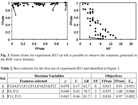
The EAFs functions were used to compare experiments H04, H06, H08 and H09 (due to a lack of space these results were presented in the supplementary informa-tion page identified above). This analysis allowed concluding that the best per-formance is obtained with the k-fold validation method when the classifier pa-rameters are optimized simultaneously (experiment H06). Finally, the advantages of using the proposed methodology for dealing with this type of problems, is shown in Figure 3 (Pareto fronts for experiment H13). In this figure is possible to observe that the algorithm is able to converge to very good solutions since high values for TPrate were obtained simultaneously with low values for FPrate. This in-dicates that the application of a MOEA, where the features to be selected and the parameters of the SVM are optimized simultaneously, is a method with good po-tentialities for solving this type of problems. The solutions identified in this plots are presented in Table 2. These include the decision variables (features selected, and classifier parameters) and the objective values. Identical results were obtained for runs H11 and H12.
0 0.2 0.4 0.6 0.8 1 0 4 8 12 16 20 NF FP ra te 0 0.2 0.4 0.6 0.8 1 0 0.2 0.4 0.6 0.8 1 FPrate TP ra te 1 2 2 1 3 3 0 0.2 0.4 0.6 0.8 1 0 4 8 12 16 20 NF FP ra te 0 0.2 0.4 0.6 0.8 1 0 0.2 0.4 0.6 0.8 1 FPrate TP ra te 0 0.2 0.4 0.6 0.8 1 0 4 8 12 16 20 NF FP ra te 0 0.2 0.4 0.6 0.8 1 0 4 8 12 16 20 NF FP ra te 0 0.2 0.4 0.6 0.8 1 0 0.2 0.4 0.6 0.8 1 FPrate TP ra te 0 0.2 0.4 0.6 0.8 1 0 0.2 0.4 0.6 0.8 1 FPrate TP ra te 1 2 2 1 3 3
Fig. 3. Pareto fronts for experiment H13 (at left is possible to observe the solutions generated in the ROC curve domain).
Table 2. Best solutions for the first run of experiment H13 and identified in Figure 3.
Decision Variables Objectives
Sol.
Features selected γ C LR NF FPrate TPrate Fm
1 F3,F4,F11,F13,F14,F16,F18,F22 0.078 0.17 62.7 8 0.013 0.91 0.951
2 F4, F11 0.040 0.43 78.7 2 0.975 1.00 0.886
3 F11, F13 0.043 0.46 81.7 2 0.818 0.97 0.892
5. Conclusions
In this work a MOEA was used for feature selection in data mining problems us-ing a Support Vector Machines classifier. The methodology proposed was able not only to propose solutions with a few number of features necessary but is able also to provide relevant information to the decision maker, such as the best features to be used but, the best parameters of the classifier and the trade-off between the dif-ferent objectives used. Finally, the approach followed here showed good potenti-alities in obtaining a good approximation to the ROC curves.
6. References
1. Guyon I, Gunn S, Nikravesh M, Zadeh, L (2006) Feature Extraction Foundations and Appli-cations. Springer.
2. Bi J (2003) Multi-Objective Programming in SVMs, Proceedings of the Twentieth Interna-tional Conference on Machine Learning, ICML-2003, Washington DC.
3. Igel C (2005) Multi-Objective Model Selection for Support Vector Machines, in C.A. Coello Coello et al. (Eds.), EMO 2005, pp. 534-546, Springer-Verlag Berlin Heidelberg.
4. Oliveira LS, Morita M, Sabourin R(2006) Feature Selection for Ensembles Using the Multi-Objective Optimization Approach, Studies in Computational Intelligence, 16:49-74.
5. Hamdani TM, Won JM, Alimi AM, Karray F (2007) Multi-objective Feature Selection with NSGA II. in Adaptive and Natural Computing Algorithms, B. Beliczynski, A. Dzielinski, M. Iwanowski, B. Ribeiro (Eds.), 8th International Conference, ICANNGA 2007, Part I, Springer-Verlag. Lecture Notes in Computer Science vol. 4431, pp. 240-247.
6. Deb K, Pratap A, Agarwal S, Meyarivan T (2002) A fast and elitist multi-objective genetic algorithm: NSGA-II,” IEEE Transaction on Evolutionary Computation, 6:181-197.
7. Alfaro-Cid E, Castillo PA, Esparcia A, Sharman K, Merelo JJ, Prieto A, Mora AM, Laredo JL (2008) Comparing Multiobjective Evolutionary Ensembles for Minimizing Type I and II Errors for Bankruptcy Prediction, Congress on Evolutionary Computation - CEC'2008, pp. 2907-2913, Washington, USA, 2008.
8. Handl J, Knowles J (2006) Feature subset selection in unsupervised learning via multiobjec-tive optimization, International Journal of Computational Intelligence Research, 2:217-238. 9. Mendes F, Duarte J, Vieira A, Ribeiro B, Ribeiro A , Neves J, Gaspar-Cunha A (2010)
Fea-ture Selection for Bankruptcy Prediction: A Multi-Objective Optimization Approach, Interna-tional Journal of Natural Computing Research , submitted for publication.
10. Kulkarni A, Jayaraman VK, Kulkarni VD (2004) Support vector classification with parame-ter tuning assisted by agent-based technique, Comp. and Chemical Engineering, 28:311–318. 11. Caruana R, Niculescu-Mizil A (2004) Data Mining in Metric Space: An Empirical Analysis
of Supervised Learning Performance Criteria, in Proc. Internat. Conf. on Knowledge Discov-ery and Data Mining, Seattle, Washington, pp. 69-78.
12. Provost F, Fawcet T (1997) Analysis and Verification of Classifier Performance: Classifica-tion under Imprecise Class and Cost DistribuClassifica-tions, in Proc. Internat. Conf. on Knowledge Discovery and Data Mining (KDD-97), Menlo Park, CA, pp. 43–48.
13. Fawcet T (2006) An introduction to ROC analysis, Pattern Recognition Letters ,27: 861–874. 14. Gaspar-Cunha A, Covas JA (2004) - RPSGAe - A Multiobjective Genetic Algorithm with
Elitism: Application to Polymer Extrusion, in Metaheuristics for Multiobjective Optimisa-tion, vol. 535, X. Gandibleux, M. Sevaux, K. Sörensen and V. T'kindt (Eds.), Lecture Notes in Computer Science, Berlin, Springer Verlag, pp. 221-249.
15. Gaspar-Cunha A (2009) Modelling and Optimization of Single Screw Extrusion, Published doctoral dissertation, 2000, in Modelling and Optimization of Single Screw Extrusion: Using Multi-Objective Evolutionary Algorithms, A. Gaspar-Cunha, Köln, Germany: Lambert Aca-demic Publishing.
16. Cortes C, Vapnik V (1995) Support-Vector Networks, Machine Learning, 20: 273-297. 17. Chang CC, Lin CJ (2000) LIBSVM a library for support vector machines (Tech. Rep.),
De-partment of Computer Science and Information Engineering, National Taiwan University, Taipei, Taiwan.
18. Kurgan LA, Cios KJ, Tadeusiewicz R, Ogiela M, Goodenday LS (2001) Knowledge Discov-ery Approach to Automated Cardiac SPECT Diagnosis, Artificial Intelligence in Medicine, 23: 149-169,.
19. Asuncion A, Newman DJ (2007) UCI Machine Learning Repository, Irvine, CA: University of California, School of Information and Computer Science. http://www.ics.uci.edu/~mlearn/MLRepository.html. Accessed 10 February 2010.
20. Fonseca C, Fleming PJ (1996) On the performance assessment and comparison of stochastic multiobjective optimizers, in Parallel Problem Solving from Nature-PPSN IV, Lectures Notes in Computer Science, Springer-Verlag, pp. 584-593.
21. Fonseca VG, Fonseca C, Hall A (2001) Inferential performance assessment of stochastic optimisers and the attainment function, in Evolutionary Multi-Criterion Optimization, Lec-ture Notes in Computer Science, Springer-Verlag, pp. 213-225.
22. López-Ibañez M, Paquete L, Stützle T (2006) Hybrid population based algorithms for the bi-objective quadratic assignment problem, in Journal of Mathematical Modelling and Algo-rithms, 5:111-137.