A Nonlinear Harmonic Balance Solver for an
Implicit CFD Code: OVERFLOW 2
by
Chad H. Custer
Department of Mechanical Engineering and Materials Science Duke University
Date:
Approved:
Dr. Earl H. Dowell, Co-advisor
Dr. Jeffrey P. Thomas, Co-advisor
Dr. Kenneth C. Hall
Dr. Donald B. Bliss
Dr. Laurens E. Howle
Dr. Zbigniew J. Kabala
Dissertation submitted in partial fulfillment of the requirements for the degree of Doctor of Philosophy in the
Department of Mechanical Engineering and Materials Science in the Graduate School of Duke University
Abstract
( Mechanical Engineering )
A Nonlinear Harmonic Balance Solver for an Implicit CFD
Code: OVERFLOW 2
by
Chad H. Custer
Department of Mechanical Engineering and Materials Science Duke University
Date:
Approved:
Dr. Earl H. Dowell, Co-advisor
Dr. Jeffrey P. Thomas, Co-advisor
Dr. Kenneth C. Hall
Dr. Donald B. Bliss
Dr. Laurens E. Howle
Dr. Zbigniew J. Kabala
An abstract of a dissertation submitted in partial fulfillment of the requirements for the degree of Doctor of Philosophy in the
Department of Mechanical Engineering and Materials Science in the Graduate School of Duke University
Copyright c 2009 by Chad H. Custer All rights reserved
Abstract
A National Aeronautics and Space Administration computational fluid dynamics code, OVERFLOW 2, was modified to utilize a harmonic balance solution method. This modification allows for the direct calculation of the nonlinear frequency-domain solution of a periodic, unsteady flow while avoiding the time consuming calculation of long physical transients that arise in aeroelastic applications.
With the usual implementation of this harmonic balance method, converting an implicit flow solver from a time marching solution method to a harmonic balance solution method results in an unstable numerical scheme. However, a relatively simple and computationally inexpensive stabilization technique has been developed and is utilized. With this stabilization technique, it is possible to convert an existing implicit time-domain solver to a nonlinear frequency-domain method with minimal modifications to the existing code.
This new frequency-domain version of OVERFLOW 2 utilizes the many features of the original code, such as various discretization methods and several turbulence models. The use of Chimera overset grids in OVERFLOW 2 requires care when implemented in the frequency-domain. This research presents a harmonic balance version of OVERFLOW 2 that is capable of solving on overset grids for sufficiently small unsteady amplitudes.
Contents
Abstract iv List of Tables ix List of Figures x Acknowledgements xiii 1 Introduction 1 1.1 Previous Research . . . 2 1.2 Research Contributions . . . 3 1.3 Outline . . . 42 Time-Domain Computational Fluid Dynamics (CFD) Model 6 2.1 Governing Equations . . . 6 2.1.1 Conservation of Mass . . . 7 2.1.2 Conservation of Momentum . . . 8 2.1.3 Conservation of Energy . . . 9 2.1.4 Equation of State . . . 10 2.1.5 Vector Form . . . 11 2.1.6 Generalized Coordinates . . . 11 2.1.7 Exact Solutions . . . 14
2.2 Finite Differencing in Space and Time . . . 16
2.2.2 Spatial Discretization . . . 25
2.3 Turbulence Modeling . . . 28
2.3.1 Reynolds Averaging . . . 29
2.3.2 Spalart-Allmaras . . . 31
3 Harmonic Balance Solution Method for CFD Model 34 3.1 Derivation . . . 35
3.2 Stability Analysis . . . 40
3.2.1 Source Term Included in the n Pseudo-time Level . . . 41
3.2.2 Source Term Included in the n+1 Pseudo-time Level . . . 47
3.3 Stabilization Technique Derivation . . . 49
3.4 Stabilized Implicit Harmonic Balance Method . . . 51
4 Time-Domain OVERFLOW 2 53 4.1 Background and History . . . 54
4.2 Chimera Overset Grids . . . 56
4.3 Force and Moment Calculation . . . 60
4.4 Aerodynamics of the AIM-120 Missile . . . 61
4.4.1 CFD Model . . . 64
4.4.2 Analytical Model . . . 65
4.4.3 Hybrid Model . . . 66
5 Capability Enhancement of OVERFLOW 2 67 5.1 Harmonic Balance Solution Method . . . 67
5.1.1 Pre-processing Phase Modifications . . . 68
5.1.2 Iteration Phase Modifications . . . 71
5.1.3 Post-processing Phase Modifications . . . 75
5.2 Time-Domain Deforming Grid Capabilities . . . 79
5.2.1 Pre-processing Phase Modifications . . . 81
5.2.2 Iteration Phase Modifications . . . 81
5.2.3 Post-processing Phase Modifications . . . 83
6 Results 84 6.1 AIM-120 Missile Aerodynamics . . . 84
6.2 Capability Enhancement Validation . . . 90
6.2.1 Parametric Convergence . . . 90
6.2.2 Comparison of Solution Methods . . . 99
6.3 Unsteady Aerodynamics of the NACA 0012 Airfoil . . . 105
6.4 F-16 Wing Modal Aerodynamics . . . 114
7 Conclusions 120 7.1 Research Contributions . . . 120
7.2 Future Work . . . 124
A Overflow 2.1 Capabilities 126
B Alternate Derivation of the HB Stabilization Technique 131
Bibliography 133
List of Tables
List of Figures
2.1 Control Volume, V bounded by the control surface, S. . . 7 2.2 Transformation of a airfoil computational domain to a generalized
coordinate system. . . 12 2.3 Couette flow. . . 15 2.4 Discretization of a two-dimensional rectangular domain. . . 16 2.5 Control surface where flux terms are evaluated with Godunov methods. 27 2.6 Wave solutions of the Riemann problem. . . 27 3.1 Airfoil location at each sub-time level of a three harmonic calculation. 39 3.2 Eigenvalues of the frequency-domain backward difference method with
the source included on the n pseudo-time level. One harmonic re-tained,ω∆t = 0.5, andλ = 0.5. . . 45 3.3 Eigenvalues of the frequency-domain Euler implicit method with the
source included on the n pseudo-time level. One harmonic retained, ω∆t = 0.5, and λ= 1.0. . . 46 3.4 Amplification factor of the frequency-domain backward difference method
with the source included on then+1 pseudo-time level. One harmonic retained, ω∆t = 0.5, and λ= 0.95. . . 49 3.5 Amplification factor of the frequency-domain Euler implicit method
with the source included on then+1 pseudo-time level. One harmonic retained, ω∆t = 0.5, and λ= 1.0. . . 50 4.1 Development history of OVERFLOW 2. Figure adapted from
OVER-FLOW 2.1 Manual [1]. . . 55 4.2 Computational grid for a regular cube. . . 57 4.3 Set of Chimera overset grids describing the NACA 0012 airfoil. . . 59
4.4 System of grids describing a sphere before and after FOMOCO
pro-cessing. . . 62
4.5 AIM 120 missile. . . 63
4.6 Surface grids of the AIM-120 missile near the forward fins. . . 64
4.7 Dimensions of the AIM-120 used for the slender body formulation of Eq. 4.1. . . 65
4.8 AIM-120 at a steady angle of attack. . . 66
5.1 Harmonic balance method flow chart. . . 69
5.2 Cartesian off-body grid corresponding to three sub-time levels. . . 78
5.3 Source term calculation for sub-time level solutions with holes. Black boxes represent data missing due to grid holes. . . 79
5.4 Fringe point communication at two sub-time levels using the single connection method. . . 80
5.5 Deforming F-16 fighter wing. . . 82
6.1 Steady aerodynamic response of the AIM-120. In Fig. 6.1(b) solid lines correspond to calculations performed on the full geometry and symbols correspond to hybrid model calculations. . . 86
6.2 Coefficient of pressure on the AIM-120 surface and near the forward fins. . . 87
6.3 Mach contours of the AIM-120 at 2◦ angle of attack. . . 88
6.4 Set of overset grids describing the NACA 0012 airfoil. . . 91
6.5 NACA 0012 unsteady coefficient of lift history calculated on a single-block c-grid with the time-domain solver. . . 94
6.6 NACA 0012 unsteady pressure along the airfoil chord calculated on a single-block c-grid with the time-domain solver. . . 95
6.7 NACA 0012 unsteady coefficient of lift history calculated on a single-block c-grid with the harmonic balance solver. . . 97
6.8 NACA 0012 unsteady pressure along the airfoil chord calculated on a single-block c-grid with the harmonic balance solver. . . 98
6.9 NACA 0012 unsteady coefficient of lift history calculated on an overset
grid with the harmonic balance solver. . . 100
6.10 NACA 0012 unsteady pressure along the airfoil chord calculated on an overset grid with the harmonic balance solver. . . 101
6.11 NACA 0012 unsteady coefficient of lift history as calculated with time-domain and frequency-time-domain methods. . . 103
6.12 NACA 0012 unsteady pressure along the airfoil chord as calculated with time-domain and frequency-domain methods. . . 104
6.13 Mach contours about the NACA 0012 airfoil at sub-time levels within one period of motion calculated on the single and overset grids at M∞= 0.5. Figure continued from previous page. . . 108
6.14 Comparison of single- and multi-block grid solutions for a pitching NACA 0012 airfoil at M = 0.5. Symbols correspond to single-block grid calculations and lines correspond to multi-block grid calculations. 109 6.15 Comparison of single- and multi-block grid solutions for a pitching NACA 0012 airfoil at M = 0.8. Symbols correspond to single-block grid calculations and lines correspond to multi-block grid calculations. 111 6.16 Mach contours about the NACA 0012 airfoil at sub-time levels within one period of motion calculated in the single grid and overset grids at M∞= 0.8. Figure continued from previous page. . . 113
6.17 F-16 fighter. . . 114
6.18 F-16 fighter wing computational grid. . . 115
6.19 Time-domain parametric convergence verification. . . 116
6.20 Frequency-domain parametric convergence verification. . . 117
6.21 Absolute and change in unsteady modal force on the F-16 wing as a function of total iterations. . . 118
Acknowledgements
I wish to express my most sincere gratitude to my advisor, Dr. Dowell. I am very fortunate to have an advisor as knowledgeable and capable as he, however it is his skill as a mentor that sets him apart.
Each of my committee members have played an important roll in this research and also deserve recognition. They are: Dr. Jeff Thomas, Dr. Kenneth Hall, Dr. Donald Bliss, Dr. Laurens Howle, Dr. Zbigniew Kabala, and Dr. Daniella Raveh. Jeff, Daniella, Dr. Hall and Dr. Dowell have been critical to the progress of this work. Their tireless support and thoughtful insight is certainly appreciated.
Thank you to Dr. Russ Rausch of the NASA Langley Research Center for his generous advisement and support. Dr. Rausch has supported my final two years of research under a NASA Graduate Student Research Program Fellowship.
I would also like to thank my family. This PhD is the product of the encourage-ment of my mom and dad. Finally, I want to thank my wife Laura. Her love and support is has sustained me.
1
Introduction
Aeroelasticity is the interaction of a structure with the fluid through which it is pass-ing. For many problems of interest, this fluid-structure interaction is unwelcome and stands as a design challenge that must be addressed. The F-16 fighter, for example, is notorious for experiencing flutter and limit cycle oscillations (LCO). Flutter is the dynamic instability of the aeroelastic (fluid-structure) system and LCO is the non-linear oscillation that may follow. These aeroelastic effects not only adversely affect the comfort and performance of the pilot, but also can lead to structural fatigue and failure [2]. Additionally, the aeroelastic behavior of the fighter is highly sensitive to a host of parameters such as aircraft configuration, flight altitude and flight speed [3]. Although the F-16 was introduced to service in 1974 [4], the aeroelastic challenges associated with the F-16 persist, which speaks to the difficulty of the problem. A key component of modeling the aeroelastic behavior of a body is the ability to model the corresponding unsteady aerodynamics accurately. The aerodynamic governing equations take the form of a set of nonlinear partial differential equations (PDEs), for which no exact solution generally exists. However, these governing equations can be discretized, forming a large system of algebraic equations that can be solved using
time-marching techniques.
The drawback of time-marching numerical schemes is that the computational cost is great. The physical transient of aeroelastic calculations tends to be very long meaning that a vast number of time steps must be modeled. Fortunately, it is possible to avoid calculating these long physical transients and instead calculate the periodic response directly by working in the frequency-domain. Additionally, the nonlinear frequency-domain harmonic balance (HB) method developed by Hall et al. [5] allows for the numerical schemes and computational grid methods developed for time-domain analysis to be used in the frequency-domain.
1.1
Previous Research
Significant work has been done with the nonlinear frequency-domain harmonic bal-ance method of Hall. The method was originally developed for turbomachinery computations [5] and have been widely used in that field to study phenomena such as non-synchronous vibration [6] and aeroelastic fan stability [7]. The method has also been extended to allow for flow fields that may be aperiodic in time [8].
In addition to turbomachinery applications, the HB method has been used ex-tensively to study the aeroelastic properties of airfoils and wings such as the NACA 64A010A [9], the NRL 7301 [10], and the AGARD 445.6 [11, 12]. Flutter and LCO calculations for the F-16 has been performed using slender body/slender wing the-ory to model stores [13]. Recently, helicopter rotors in hover and forward flight have been modeled using the HB method [14]. Also, the HB method has been used in conjunction with shape design optimization [15–17].
Advancement of the harmonic balance method continues and it has been used in conjunction with acceleration techniques originally intended for time-domain meth-ods [18]. Research has been done on systems with time perimeth-ods that are either variable or unknown a priori [19, 20]. Also, a recent paper explores using overset
grids with a frequency-domain method [21].
1.2
Research Contributions
The objective of this research is to create a harmonic balance implementation of the time-domain computational fluid dynamics (CFD) solver OVERFLOW 2, which employs advanced implicit discretization techniques, uses robust turbulence models and is capable of solving on Chimera overset grids. In achieving this objective the following research contributions are made.
Development of a novel stabilization technique that allows the harmonic balance method to be used in conjunction with implicit finite difference methods.
A simple and computationally efficient numerical stabilization technique is devel-oped. This technique allows for the form of the linear system that must be solved to mimic that of the time-domain, while retaining the stability requirements of the original time-domain scheme.
Implementation of the harmonic balance method about the existing time-domain CFD solver OVERFLOW 2.
OVERFLOW 2 is a time-domain flow solver with many advanced discretization techniques and turbulence models implemented. A full list of features is given in Ap-pendix A. The nonlinear frequency-domain harmonic balance method is implemented about OVERFLOW 2. This new solver is capable of using a suite of finite difference techniques and turbulence models and is shown to perform accurate unsteady modal aerodynamic calculations.
balance version of OVERFLOW 2.
Modeling the geometry of interest accurately is shown to be important for cal-culating the aerodynamics of complex bodies. To allow for accurate geometric rep-resentation of bodies such as a fighter aircraft, a Chimera overset grid technique is integrated into the harmonic balance implementation of OVERFLOW 2.
Incorporate deforming grid capabilities into the time-domain version of OVERFLOW 2.
Deforming grid capabilities are introduced to time-domain OVERFLOW 2, al-lowing for the validation of the HB implementation of OVERFLOW 2. Also, time-domain and frequency-time-domain versions of the same solver allow timing studies to be performed. Finally, the time-domain deforming grid version of OVERFLOW 2 can be used to model scenarios where physical transients are important such as aircraft maneuver simulations.
1.3
Outline
First, the mathematical foundation for the work to follow is presented. Chapter 2 describes the equations that govern fluid dynamics as well as the discretization techniques that will be used in this research. Chapter 3 describes the nonlinear frequency-domain representation of the governing equations. This chapter also ex-amines the stability of various implementations of the harmonic balance method using the 1-D advection equation. The final portion of Chapter 3 develops a novel stabilization technique for the harmonic balance method.
Next, Chapter 4 gives background on the time-domain CFD solver OVERFLOW 2 and describes three aerodynamic models for the AIM-120 missile. These models are created to determine the level of geometric complexity required to model a modern fighter aircraft complete with stores.
Chapter 5 describes the modifications required to transform OVERFLOW 2 from a time-domain solver to a nonlinear frequency-domain solution method. This chapter also develops a method for using Chimera overset grids with the HB implementation of the solver. Finally, modifications to the time-domain version of OVERFLOW 2 that allow for deforming grids are described.
The results from the models and methods developed in Chapters 4 and 5 are presented in Chapter 6. First, the solutions produced by the three aerodynamic models of the AIM-120 are presented. It is shown that a full geometric representation of the body is required to capture accurately the aerodynamic response of a complex body. Next, the capabilities implemented in Chapter 5 are validated by comparing solutions computed for a transonic NACA 0012 airfoil oscillating in pitch. Finally, time-domain and frequency-domain results for a deforming F-16 wing at a Mach number of 0.9 are presented.
Research contributions are highlighted in Chapter 7 and the document closes with suggestions for future work.
2
Time-Domain
Computational
Fluid
Dynamics
(CFD) Model
2.1
Governing Equations
The Navier-Stokes equations, named for Claude-Louis Navier and George Gabriel Stokes, are a set of nonlinear partial differential equations (PDEs), which state that the momentum of an infinitesimal volume of compressible, viscous fluid must be conserved [22]. Together with equivalent statements concerning the conservation of mass and energy, a set of equations is formed, which govern fluid flow. Although the Navier-Stokes equations formally refer to the conservation of momentum equations, the name is used often to refer to the entire set of governing equations.
Since this set of equations describes such a vast array of physical systems, many disciplines are interested in their solution. Along with topics in aerodynamics and aeroelasticity, the Navier-Stokes equations are critical to the study of acoustics [23, 24], biology [25], hydrodynamics [26], meteorology [27] and astrophysics [28, 29], to name a few.
These governing equations are based on a few basic assumptions about the fluid. It is assumed that the fluid is a homogeneous continuum in which there are no
chem-ical reactions or mass diffusion. It is possible to add terms in order to allow for chemically reacting flows [30], however all flows considered here are non-reacting. In deriving the governing equations, it also assumed that the field quantities and their derivatives are continuous, at least in the weak sense. The following sections will explore each conservation equation and point out the basic features of the equa-tions. Numerous derivations of the governing equations have been published over the years [31–33]. Tannehill et al. [34] is a favorite reference, and was often consulted for the writing of the following sections.
2.1.1 Conservation of Mass
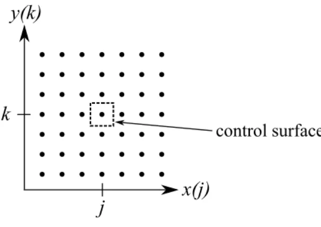
The conservation of mass principle simply states that mass is neither created nor destroyed. When this principle is applied to a fluid, the resulting equation is known as the continuity equation. The continuity equation can be derived by considering a Eulerian control volume at rest within the flow field, as shown in Fig. 2.1. Since
Figure 2.1: Control Volume, V bounded by the control surface, S.
mass can be neither created nor destroyed, the continuity equation states that the rate of change of the mass of the fluid within the control volume is balanced by the mass flux through the boundary of the control volume.
∂ρ
The fluid density is represented by ρ, and V describes the velocity field of the fluid. It is often convenient to work in terms of the substantial derivative given by Eq. 2.2.
D() Dt ≡
∂()
∂t +V· ∇() (2.2)
The substantial derivative describes the time rate of change of a quantity as a fluid element moves within the flow. When written in terms of the substantial derivative, the continuity equation becomes the following.
Dρ
Dt +ρ(∇ ·V) = 0 (2.3)
2.1.2 Conservation of Momentum
Newton’s Second Law, as given by Eq. 2.4, states that the time rate of change in momentum of an object is equal to the force applied.
F= dp
dt (2.4)
HereF is the force applied, and p is the momentum of the object.
This same concept is used to derive the conservation of momentum equation. Although the resulting expression is much more complex than Newton’s Second Law, the concept is fairly simple. The change in momentum of the infinitesimal fluid volume is due to body forces, viscous stresses and convection through the surface of the control volume. In the conservation of momentum equation, given by Eq. 2.5, f
represents the body force per unit mass.
ρDV
Dt =ρf +∇ ·Πij (2.5)
The surface forces, which consist of normal and shear stresses, are given by Eq. 2.6 for a Newtonian fluid.
The viscous stress tensor is given by τij. τij=µ ∂ui ∂xj + ∂uj ∂xi − 2 3δij ∂uk ∂xk (2.7)
The viscosity of the fluid is given byµ, andδij is the Kronecker delta function. The
velocity in each coordinate direction is given by ui,j,k and the coordinate directions
themselves are xi,j,k.
By substituting Equations 2.6 and 2.7 into Eq. 2.5, the Navier-Stokes equation is formed. ρDV Dt =ρf − ∇p+ ∂ ∂xj µ ∂ui ∂xj + ∂uj ∂xi − 2 3δijµ ∂uk ∂xk (2.8) 2.1.3 Conservation of Energy
The conservation of energy statement is derived from the First Law of Thermody-namics given by Eq. 2.9.
∆Et =Q−W (2.9)
Equation 2.9 states that the change in total internal energy of a system (∆Et) is
equal to the energy transfer by heat into the system (Q) minus the work done by
the system (W).
Like the previous derivations, the conservation of energy equation is derived by applying the applicable basic principle to the control volume within the fluid. The total energy per unit volume of the fluid is equal to the internal energy per unit mass (e) plus the kinetic energy per unit volume (K) and potential energy per unit volume (U) of the fluid.
Et=ρ(e+K+U) (2.10)
The conservation of energy equation is given by Eq. 2.11.
∂Et
∂t +∇ ·EtV= ∂Q
The left hand side of the equation represents the change in energy of the system and the convection of energy through the surface of the control volume. The first term on the right is the rate of heat produced while the second term quantitates the amount of heat lost from the control volume due to convection. Note that k is the thermal conductivity and T is the temperature of the fluid. The final two right hand terms represent the work doneon the system by body forces and surface forces, respectively.
2.1.4 Equation of State
The previous sections of this chapter outline the fundamental governing equations of fluid flow. However, the equations above do not form a closed system. That is to say that there are more unknown variables than there are equations. The independent variables of Equations 2.1, 2.8, 2.11 are pressure, three components of velocity, temperature, density and internal energy. For these seven variables there are only five equations.
It is often assumed that the fluid in question obeys the Perfect Gas Law,
p=ρRT (2.12)
where R is the gas constant.
In addition we will assume that the fluid is calorically perfect meaning that the specific heat at a constant volume (cp) and the specific heat at a constant temperature
(cv) are unchanging. This allows us to write pressure and temperature as a function
of internal energy and density.
T = (γ−1)e R (2.13) p= (γ−1)ρe (2.14) γ = cp cv (2.15)
Using these equations of state, pressure and temperature are no longer indepen-dent variables. This closes the system and leaves five equations for five unknowns.
2.1.5 Vector Form
It is convenient to formulate this system of equations into a single vector equation. For the Cartesian coordinate system, the vector equation is given by
∂U ∂t + ∂E ∂x + ∂F ∂y + ∂G ∂z =0 (2.16) where U = ρ ρu ρv ρw Et (2.17) E = ρu ρu2+p−τ xx ρuv−τxy ρuw−τxz (Et+p)u−uτxx−vτxy −wτxz+qx (2.18) F = ρv ρuv−τxy ρv2+p−τ yy ρvw−τyz (Et+p)v−uτxy −vτyy−wτyz+qy (2.19) G = ρw ρuw−τxz ρvw−τyz ρw2+p−τzz (Et+p)w−uτxz −vτyz−wτzz+qz (2.20) 2.1.6 Generalized Coordinates
It is often easier to formulate computational methods from the Cartesian vector form of the Navier-Stokes equations. However, most flow solvers do not operate in the
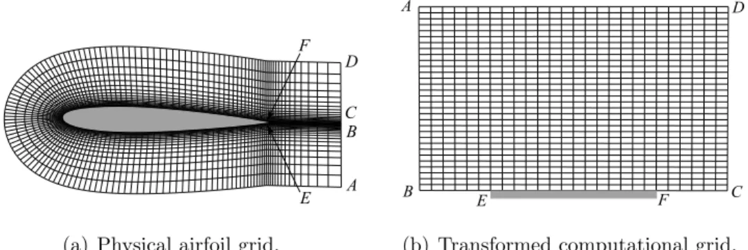
Cartesian coordinate system. Instead, complex computational grids are transformed onto a regular geometry. This concept is illustrated in Fig. 2.2 where the domain surrounding an airfoil is transformed to a regular geometry.
(a) Physical airfoil grid. (b) Transformed computational grid.
Figure 2.2: Transformation of a airfoil computational domain to a generalized coordinate system.
The generalized coordinates of the computational domain (ξ, η, ζ) can be ex-pressed in terms of the Cartesian coordinates (x, y, z) illustrated in Eq. 2.21.
ξ = ξ(x, y, z)
η = η(x, y, z) (2.21)
ζ = ζ(x, y, z)
Using the chain rule, Eq. 2.22 transforms from the geometric space to the computa-tional space. dξ dη dζ = ξx ξy ξz ηx ηy ηz ζx ζy ζz dx dy dz (2.22)
Likewise, Eq. 2.23 transforms from the computational space to the geometric space.
dx dy dz = xξ xη xζ yξ yη yζ zξ zη zζ dξ dη dζ (2.23)
By setting Eq. 2.22 equal to Eq. 2.23, the transformation metrics can be found. ξx ξy ξz ηx ηy ηz ζx ζy ζz =J yηzζ−yζzη −(xηzζ−xζzη) xηyζ−xζyη −(yξzζ−yζzξ) xξzζ−xζzξ −(xξyζ−xζyξ) yξzη−yηzξ −(xξzη−xηzξ) xξyη −xηyξ (2.24)
Where the Jacobian (J) is given by:
J = ∂(ξ, η, ζ) ∂(x, y, z) = ξx ξy ξz ηx ηy ηz ζx ζy ζz = 1 J−1 = 1/ ∂(x, y, z) ∂(ξ, η, ζ) = 1 xξ xη xζ yξ yη yζ zξ zη zζ
The transformation metric can be calculated analytically if there is a known ex-pression for the inverse transformation, however this is rarely the case. Generally, the transformation metrics will be computed by approximating the derivatives using finite difference techniques.
The final step of this section is to consider the governing equations in generalized coordinates. As shown in Eq. 2.25, the form of the equations does not change from that of Eq. 2.16. ∂Uˆ ∂t + ∂Eˆ ∂ξ + ∂Fˆ ∂η + ∂Gˆ ∂ζ =0 (2.25)
ˆ U = 1 JU ˆ E = 1 J(Eξx+Fξy +Gξz) ˆ F = 1 J(Eηx+Fηy +Gηz) ˆ G = 1 J(Eζx+Fζy +Gζz) 2.1.7 Exact Solutions
The Navier-Stokes equations are a set of nonlinear partial differential equations for which there exists no general solution. In fact it has not yet been proven that there always exists a solution to the three-dimensional Navier-Stokes equations. This is known as the Naiver-Stokes existence and smoothness problem [35]. Since it is rarely possible to find analytical solutions to the governing equations, alternate techniques must be employed. It is for this reason that computational fluid dynamics has become an extremely popular method for solving all but the simplest of flows.
There are, however, a small class of flows for which exact solutions can be found. Some examples include steady channel flow, steady flow into a corner, and steady flow of a circular pipe [36].
As a representative example, this section will discuss the solution to Couette flow [37]. Consider a fluid between two infinite flat plates separated by a distanceh with the top plate moving at a velocity of utop and the bottom plate fixed. This
scenario is illustrated in Fig. 2.3. Due to the infinite nature of the plates, the Navier-Stokes equation given by Eq. 2.8 are only y−dependent for this configura-tion. Additional assumptions such as no body forces acting on the fluid and no pressure gradients result in a greatly simplify equation describing x velocity of the
Figure 2.3: Couette flow. flow. ∂ ∂y µ∂u ∂y = 0 (2.26)
With the added assumption that the viscosity, µ, is unchanging, we are able solve this equation by simply integrating twice. The constants of integration are found by enforcing the following boundary conditions at the upper and lower walls.
u(y= 0) = 0, u(y=h) =utop (2.27)
The solution, as given by Eq. 2.28, shows that the velocity profile is a linear function of y.
u(y) = utop y
h (2.28)
Clearly, this example is far less complex than most problems of interest. Typi-cally exact solutions are only possible when both geometry and assumptions about the flow result in many terms within the governing equations equaling zero. In fact, if variable fluid properties are considered for the same geometry as above, computa-tional methods must be employed [38].
Although there exist special cases, such as Couette flow, for which exact solu-tions can be found, this is not an option for most flows of interest. The geometries considered will generally be highly complex, allowing for no canceling of terms. Also,
simplifying assumptions about the flow, such as incompressibility, will not be made. For these reasons CFD methods are by far the most common method for solving flow fields. There exist challenges and shortcomings with CFD methods as well, however it is the only practical method for solving complex flow fields.
2.2
Finite Differencing in Space and Time
Instead of trying to solve for the continuous functions that describe the conservation variables within the flow domain, the region of interest is discretized. As such, the solution is only considered at a finite number of points within the domain. A discretization of a two-dimensional plane is shown in Fig. 2.4, where each point represents a location at which the governing equations will be solved. The governing equations will only be solved at these discrete points within the domain.
Figure 2.4: Discretization of a two-dimensional rectangular domain.
Since we are no longer seeking continuous functions of the conservation variables as solutions, the partial differential equations governing the system are converted into a system of algebraic equations. This conversion is achieved by approximating the spatial and temporal derivative operators of the governing equations. The
ap-proximations are often based on the very definition of a derivative, given in Eq. 2.29.
du
dx = lim∆x→0
u(x)−u(x−∆x)
∆x (2.29)
Since there is some finite distance between any two given nodes, say ∆xj, this limit
cannot go to zero. The finite difference approximation most closely corresponding to Eq. 2.29 is known as backward differencing.
∂u ∂x j ≈ uj −uj−1 ∆xj (2.30)
The backward differencing method is one of the simplest approximations. This tech-nique only uses information from the node where the derivative will be calculated and the neighboring node in one direction to calculate the derivative. There are a vast number of finite difference approximations in use today; each designed for a par-ticular purpose [34, 39]. For example, when there is a known direction of information travel, the derivative approximation will include the nodes from which information is naturally propagated. The collection of nodes used to calculate the derivative is known as the stencil. The stencil shown Fig. 2.4 is a central difference method, taking information from each of the neighboring nodes.
Recall that the governing equations also contain a time derivative term, meaning that time will be discretized in the same fashion as space. Since time is no longer a continuous function, one must choose on what time level to evaluate the spatial derivative terms; the current time-level (n) or the future time-level (n + 1). If the spatial derivatives are evaluated on the n time-level the resulting scheme isexplicit, whereas if the derivatives are evaluated on then+ 1 time-level the scheme isimplicit. As an example, consider the simple advection equation, ut+aux = 0. An explicit
discretization would be unj+1−unj ∆t +a un j −unj−1 ∆x = 0 (2.31)
whereas an implicit discretization would be unj+1−un j ∆t +a unj+1−unj−1+1 ∆x = 0. (2.32)
Both methods form a linear system that takes the following form.
[A]un+1 = [B]un. (2.33)
The distinguishing feature is that with explicit methods [A] is a diagonal matrix, whereas with implicit methods it is not.
There are an unlimited number of finite difference approximations that can be constructed, however all must be consistent with the equation being approximated.
Consistency and Order of Accuracy
After creating a finite difference approximation to a partial differential equation, it is important to ensure that the PDE is being represented properly. This property is known as consistency. The finite difference representation of the PDE must obey the property that as ∆x and ∆t go to zero, the exact PDE is recaptured.
This analysis is performed by Taylor expanding each of the terms of the finite difference equation (FDE) and grouping terms by powers of ∆x and ∆t. The re-sulting equation is known as the FDE’s modified partial differential equation. As an example, the modified partial differential equation for the discretization of the advection equation given by Eq. 2.31 is given by the following.
ut+aux =
∆t
2 utt+a∆xuxx (2.34)
Clearly as ∆x,∆t → 0 the advection equation results, meaning that this scheme is consistent.
With a given discretization of time and space, ∆t and ∆x will always be some finite values. On a practical level, having a consistent representation of the PDE
means that with a sufficiently small time step and sufficiently refined grid, the PDE will be modeled accurately. Unfortunately there is no method for calculating the required time step and grid size. Instead, multiple trials must be run. For example to ensuregrid convergence, computations are performed on a set of grids with increasing refinement.
The modified PDE also determines the order of accuracy of the method in ques-tion. The truncation error (Et) of a method is the difference between the PDE and
the FDE. In other words the truncation error is the sum of all terms containing pow-ers of ∆xand ∆t. The order of accuracy of a method is expressed as the lowest power of ∆xand ∆tpresent inEt. By inspecting Eq. 2.34, it is clear that this discretization
isO(∆x,∆t). This means that the truncation error scales proportionally to ∆xand ∆t. In order to reduce truncation error, higher order schemes are desirable.
Scheme Stability
A stable scheme is a scheme in which numerical errors do not grow in discrete time. Generally speaking there is some criterion involving ∆xand ∆tthat must be satisfied for a particular scheme to be stable. There is no method for directly obtaining the
stability criterion for a nonlinear PDE; instead, the equation must first be linearized. With the linearized version of the equation, a von Neumann stability analysis can be performed.
Recall that we are only considering the linearized PDE. Based on the principle of superposition, we treat the error as a superposition of waves and determine the cri-terion for which a single wave amplitude grows in time. The error can be represented as
(x, t) =rn(t)eik∆xi(x) (2.35)
and this error does not grow as long as the magnitude of the amplification factor,r, is less than or equal to unity.
Generally, the stability criteria for implicit methods are much less strict than those for explicit methods. Therefore, it is possible to take larger time steps for a given computational grid. The trade off is that there is an increased computational cost associated with solving the algebraic system for an implicit method since [A] is not diagonal. However, reduction in computational cost associated with the ability to take larger time steps usually far outweighs the cost penalty of solving the algebraic system.
This research is interested in converting an implicit time-domain CFD solver to the harmonic balance method. Although the discretization techniques are much more complex than the 1-D examples outlined above, the basis of the methods remains the same. This research will focus on converting the NASA developed CFD solver OVERFLOW 2 to the harmonic balance method. There are a vast number of dis-cretization methods implemented within OVERFLOW 2. In the following sections two temporal and spatial discretizations will be discussed. These are the methods that will be used to produce the results of this project, and so are presented for reference. However, it is important to note that the conversion of OVERFLOW 2 to the harmonic balance method is independent of the discretization techniques imple-mented.
2.2.1 Temporal Discretizations
Each of the temporal discretizations discussed in the following sections utilize sub-time iterations, which can improve sub-time marching accuracy and also results in a more stable numerical scheme [1, 40]. For a more complete discussion of the implemen-tation of sub-time iterative methods in OVERFLOW 2, the reader is directed the treatment of Pandya et al. [41]. Recall from Eq. 2.25 that the governing equations
can be represented by the following vector equation in generalized coordinates. ∂U ∂t + ∂E ∂ξ + ∂F ∂η + ∂G ∂ζ =0
For a sub-iterative scheme, a pseudo-time derivative will be added to Eq. 2.25 as given by Eq. 2.36. ∂U ∂t + ∂U ∂τ + ∂E ∂ξ + ∂F ∂η + ∂G ∂ζ =0 (2.36)
This equation can then be discretized using the Euler implicit method. In Eq. 2.37 physical time steps are indexed by n and sub-iterations are indexed by m.
I+ ∆t (1 +θ)∆τ ∆Un+1,m+1 + ∆t 1 +θ ∂ ∂ξ ∆E n+1,m+1 + ∂ ∂η ∆F n+1,m+1 + ∂ ∂ζ ∆G n+1,m+1 =− (Un+1,m−Un)− θ 1 +θ∆U n+ ∆t 1 +θRHS n+1,m (2.37)
The equation above is written in delta form, where ∆Un+1,m+1 =Un+1,m+1−Un+1,m
and corresponds to the change in the solution vector from the previous time step and sub-iteration. The order of the time differencing is controlled by θ where θ = 0 corresponds to first order time differencing andθ = 1/2 corresponds to second order time differencing. The right-hand-side term contains the spatial difference terms and is given by Eq. 2.38. RHS = ∂E ∂ξ + ∂F ∂η + ∂G ∂ζ (2.38)
Note that the pseudo-time term is discretized using first order time differencing. The delta terms of Eq. 2.37 can then be linearized by retaining the first term of the corresponding Taylor series. An example for the linearization of E follows.
En+1 =En+ ∂E ∂U n Un+1−Un+O(∆t2) (2.39)
The result is that these delta terms can be expressed in terms of a matrix multiplying the update vector, ∆Un+1.
∆En+1 = ∂E ∂U n ∆Un+1 =A∆Un+1 ∆Fn+1 = ∂F ∂U n ∆Un+1 =B∆Un+1 (2.40) ∆Gn+1 = ∂G ∂U n ∆Un+1 =C∆Un+1
Substituting these expressions into Eq. 2.37 yields the following.
I+ ∆t (1 +θ)∆τ + ∆t 1 +θ ∂A ∂ξ + ∂B ∂η + ∂C ∂ζ ∆Un+1,m+1 =− Un+1,m−Un− θ 1 +θ∆U n+ ∆t 1 +θRHS n+1,m (2.41)
With the pseudo-time step (∆τ) constant throughout the domain, Eq. 2.41 repre-sents a Newton sub-iteration scheme. If ∆τ varies throughout the domain, Eq. 2.41 represents a dual time-stepping algorithm. It is important to note that when utiliz-ing sub-iterations, the solution must be converged in pseudo-time for each physical time step in order to ensure time accuracy.
The linear system represented by Eq. 2.41 is solved implicitly on each individual grid. However, overset grid methods will be used meaning that the computational domain may contain many individual grid blocks. Information is transferred between grids in these overlapping regions explicitly. Also, the solution at nodes with specified boundary conditions is imposed explicitly. The inclusion of sub-iterations allows for better transfer of information between grid blocks, improving convergence and accuracy.
Diagonalized Beam-Warming Factored Method
Solving the linear system expressed by Eq. 2.41 can be extremely computationally expensive, especially considering the fact that modern CFD solvers will have millions of degrees of freedom. One method for reducing the resources required to solve the linear system is to factorize the linear system [1, 42, 43]. The factorization of Eq. 2.41 is given by I+ ∆t (1 +θ) ∂A ∂ξ I+ ∆t (1 +θ) ∂B ∂η I+ ∆t (1 +θ) ∂C ∂ζ ∆Un+1,m+1 =− Un+1,m−Un − θ 1 +θ∆U n+ ∆t 1 +θRHS n+1,m +Ef act (2.42)
where the error due to the factorization is given by the following.
Ef act = " ∆t 1 +θ 2 ∂A ∂ξ ∂B ∂η + ∂A ∂ξ ∂C ∂ζ + ∂B ∂η ∂C ∂ζ + ∆t 1 +θ 3 ∂A ∂ξ ∂B ∂η ∂C ∂ζ # ∆Un+1,m+1 (2.43)
The factorization shown above is known as the three factor alternating direction implicit (ADI) scheme. Since A, B and C are block tridiagonal matrices, each of the three matrices on the left-hand-side of the equation are block tridiagonal, which means that the linear system can be solved efficiently.
Subsequently, the A, B and C matrices can be decomposed into Eigenvalues and Eigenvectors as given in Eq. 2.44.
A=XAΛAXA−1
B =XBΛBXB−1 (2.44)
By commuting the eigenvalues and the differential operators, Eq. 2.42 becomes the following linear system, which is a pentadiagonal matrix system in each direction.
XA I+ ∆t (1 +θ) ∂ΛA ∂ξ XA−1XB I+ ∆t (1 +θ) ∂ΛB ∂η XB−1 XC I+ ∆t (1 +θ) ∂ΛC ∂ζ XC−1∆Un+1,m+1 =− Un+1,m−Un− θ 1 +θ∆U n+ ∆t 1 +θRHS n+1,m +Ef act (2.45)
Note that for this system, artificial second and fourth order smoothing is required. This system is less costly to solve since each of the three matrices on the left-hand-side of the equation are pentadiagonal matrices. The diagonalized Beam-Warming pentadiagonal scheme will be the standard factorized method used in this research.
Symmetric Successive Over-Relaxation Unfactored Method
The Symmetric Successive Over-Relaxation (SSOR) method [1, 43] is an unfactored method and therefore does not suffer from the factorization error as does the method above. The SSOR algorithm can be expressed as the following.
∆Uj,k,lmm+1 = (1−Ω)∆Uj,k,lmm+ Ω RHS−AL∆Ujmm−1,k,l−1 −AR∆Ujmm+1,k,l−1
−BL∆Uj,kmk−11 ,l−BR∆Uj,kmk+12,l (2.46)
−CL∆Uj,k,lml1−1−CR∆Uj,k,lml2+1
In the above equation the subscriptsL,DandU denote the lower, diagonal and upper portions of the block tridiagonal matrix. Overbars represent the premultiplication by the inverse of AD+BD+CD, and Ω is the relaxation parameter. This parameter is
typically set to 0.9, which represents an under-relaxation. Since, as the name implies, this is a symmetric and successive technique, there will be forward and backward sweeps and the sweeps will be performed multiple times in order to converge to a
solution. A forward Jacobi sweep is performed in the j direction and symmetric Gauss-Seidel sweeps are performed in the k and l directions. The forward k and l sweeps are defined as
mk1 =mm+ 1, mk2 = mm, ml1 =mm+ 1, ml2 =mm (2.47)
while the backward sweeps are defined as
mk1 =mm, mk2 =mm+ 1, ml1 =mm, ml2 = mm+ 1 (2.48)
where mmis the sweep index.
The SSOR method eliminates the factorization error, however the trade off is in increased computational cost and memory requirements. Since multiple sweeps are being performed in the method, the compute time for a physical time step is larger than the factored methods of the previous section. Also, the entire flux Jacobian must be stored. This means that the memory required is increased over that of the factored method outlined above.
The SSOR method has proven to be a robust algorithm for unsteady flows and will be used extensively in this research.
2.2.2 Spatial Discretization
The spatial discretization is responsible for approximating the derivatives within the RHS term such as in Eq. 2.45 and Eq. 2.46. As is the case with time discretizations, there are many spatial discretizations available within OVERFLOW 2. Each method offers a unique set of benefits and limitations.
Central Difference
As the name implies, central differencing techniques take information from both positive and negative directions when approximating the derivative. An example of
a second order central difference scheme is give by Eq. 2.49.
∂u ∂t ≈
uj+1−uj−1
2∆x (2.49)
The order of the approximation can be increased by including more points in the stencil. Second order through sixth order central difference schemes are available within OVERFLOW 2 [1]. However, at the boundary of overlapping grids, second order methods are always used.
Central difference methods are easy to implement and well suited for many prob-lems. However, central difference methods are not able to accurately model disconti-nuities in the domain, such as shocks. These methods tend tosmear the shock [44]. This means that the shock will not be a step discontinuity between nodes. Instead, the shock will be modeled as a large change in the conservation variables over the range of a few nodes.
HLLC Upwind
Many finite difference techniques, including the central difference scheme, are based on Taylor series approximations of derivatives. These schemes assume that the con-servation variables and their derivatives are continuous. This clearly is not the case in shock regions or near other discontinuities. To circumvent this issue, Godunov [45] proposed evaluating the flux terms of the conservation variables on a finite volume basis. This concept is illustrated in Fig. 2.5.
Godunov methods determine the flux at each cell face by employing Riemann solution techniques at each interface. The Riemann problem is the initial value problem of a set of conservation equations where a discontinuity is centered atx= 0, for the one dimensional case [46]. This initial value problem results in three types of waves as illustrated in Fig. 2.6. The right and left waves represent shocks and rarefactions, respectively, whereas the middle wave is a contact surface. The contact
Figure 2.5: Control surface where flux terms are evaluated with Godunov methods.
surface separates regions of differing temperature and density.
Figure 2.6: Wave solutions of the Riemann problem.
Harten, Lax and van Leer proposed a Godunov-type upstream differencing method that has become known as the HLL scheme [47]. The major benefit of this method is the ability to capture a sharp shock at the proper location within the flow field. Also, the method is accurate away from the shock and is robust. However, this method does not account for the contact discontinuity. The result is that discontinuities in temperature and energy within the flow field can exist, and additionally vortex sheets can be smeared [48].
Many variations to the HLL scheme have been proposed. Toro, Spruce and Spears formulated a method to restore the missing contact surface of the HLL method [48].
This method is known as the HLLC method and is implemented within OVER-FLOW 2.
2.3
Turbulence Modeling
Turbulence is a centuries’ old problem and as such much has been written on the topic [49–51]. A CFD practitioner’s guide has been developed by Nichols and pro-vided useful background in the writing of this section [52].
Turbulent flow is chaotic and non-repeating in time. It is widely accepted that the Navier-Stokes equations are fully able to model turbulent flow, however it is extremely rare that turbulent flows are modeled directly. Calculations of these types are referred to as direct numerical simulations (DNS) and have only been performed for simple geometries due to extreme computational cost [53].
DNS calculations are extremely difficult to perform because the turbulent length and time scales are much smaller than the length and time scales that are typically of interest. The smallest turbulent scale, known as the Kolmogorov scale, are given by Eq. 2.50 where λ is the length scale and τ is the time scale.
λ= ν3 1/4 , τ =ν 1/2 (2.50)
In Eq. 2.50, ν is the kinematic viscosity, and is the turbulent dissipation. These length and time scales tend to be orders of magnitude smaller than the character-istic length of the body and the time scale of the body motion. Thus, in order to fully resolve all length scales of the flow, an exorbitant number of nodes would be needed within the domain. Likewise, in order to resolve the turbulent time scale a prohibitively small time step would be needed.
2.3.1 Reynolds Averaging
Since the CFD practitioner is not usually interested in modeling the unsteady flow at the turbulent length and time scales, approximations are made that seek to model the averaged result of the small scale turbulence. A popular technique is to separate the primitive variables based on time scale [52, 54]. An example for the decomposition of a general velocity component is shown by Eq. 2.51 where the overbar indicates the time averaged portion and the prime indicates turbulent level variation.
uj(x, t) = ¯uj(x) +u0j(x, t) (2.51)
In the above equation, the averaging is done on a time scale larger than the turbulent time scale. The result is that the turbulent fluctuations are captured by primed quantities. The separated expressions for the primitive variables are then substituted into the continuity equation (Eq. 2.1), the Navier-Stokes equation (Eq. 2.8), and the conservation of energy equation (Eq. 2.11). The result of this substitution is a set of equations similar in form to the original governing equations, that are known as the Reynolds-averaged Navier-Stokes (RANS) equations.
Conservation of Mass ∂ρ¯ ∂t + ∂ ∂xj ( ¯ρu¯j) = 0 (2.52) Conservation of Momentum ∂ ∂t( ¯ρu¯i) + ∂ ∂xj ( ¯ρu¯iu¯j) + ∂ ∂xj RS z }| { ( ¯ρu¯iu¯j) = − ∂p¯ ∂xi + ∂τ¯ij ∂xj (2.53)
Conservation of Energy ∂ρ¯E¯ ∂t + ∂ ∂xj ¯ ρu¯jH¯ + ∂ ∂xj THF z }| { ¯ ρu0je0+ ¯u i RS z }| { ¯ ρu0iu0j+1 2 TDF z }| { ¯ ρu0iu0iu0j= ∂ ∂xj ( ¯ujτ¯ij) + ∂ ∂xj u0 iτij0 | {z } TDS − ∂ ∂xj κT ∂T¯ ∂xj (2.54) ¯ H = ¯E+p¯ ¯ ρ = ¯ e+1 2u¯iu¯i+ 1 2u 0 iu 0 i + p¯ ¯ ρ
The turbulent variation terms are labeled in the above equations and can be interpreted physically. The term labeled RS is the so called Reynolds stress term and represents the transport of momentum due to the turbulent motion. The turbulent heat flux is labeled as THF and the turbulent diffusion and dissipation are labeled as TDF and TDS, respectively.
With the introduction of these new unknown quantities, the RANS equations are in need of closure. The Boussinesq approximation states that the Reynolds stresses can be treated in the same manner as viscous stresses in laminar flows. As such the Reynolds stresses are modeled by
−ρu¯ 0iu0j =µt ∂ui ∂xj + ∂uj ∂xi −2 3ρkδi,j (2.55)
where µt is the eddy viscosity and k is the turbulent kinetic energy.
Using the Boussinesq approximation, the RANS equations are significantly sim-plified. The conservation of mass and conservation of momentum equations are un-changed in form from the original governing equations given by Eq. 2.1 and Eq. 2.8, respectively. The only change in these equations is that viscosity (µ) appearing in τij, as given by Eq. 2.7, includes the turbulent eddy viscosity µt. The conservation
of energy equation becomes ∂ρE ∂t + ∂ ∂xj (ρujH) = ∂ ∂xj (ujτij)− ∂ ∂xj µ P r + µt P rt ∂T ∂xj (2.56)
whereµt is the eddy viscosity and P ris the Prandtl number, a non-dimensional
pa-rameter. Note that with this simplification, the eddy viscosity is the only additional unknown to the system of equations. In order to close this system, many turbulence models have been developed.
The benefit of the Reynolds-averaging method is clear. The phenomenon of turbulence is confined to a single additional variable on the global length scale. This means that the turbulent length and time scales do not need to be modeled. This too is the limitation of the method. Since all turbulence is on a sub-grid length scale, a great deal of importance is placed on the turbulence modeling. Since turbulence is one of the unsolved problems in nature, the current models are only reliable for specific classes of flow and must be calibrated appropriately.
2.3.2 Spalart-Allmaras
The turbulence model developed by Spalart and Allmaras [52, 55] is a one-equation transport type turbulence model that has enjoyed a great deal of popularity and success for a wide variety of flows. This turbulence model will be used for the majority of the research presented. The Spalart-Allmaras (SA) turbulence model can be expressed as shown in Eq. 2.57.
∂ν˜ ∂t +Ui ∂ν˜ ∂xi = 1 σ ∇ ·[(ν+ ˜ν)∇ν˜] +Cb2(∇ν˜)2 +P(˜ν)−D(˜ν) (2.57)
Above, ˜ν is the turbulence variable and has dimensions of viscosity. The left-hand-side of the equation represents the convection of the turbulence variable and the bracketed term on the right-hand-side represents the diffusion of turbulence. P(˜ν)
and D(˜ν) are production and destruction terms. The production and destruction terms are given by the following.
P(˜ν) = Cb1ν˜ Ω + ν˜ κ2d2fν2 (2.58) D(˜ν) =Cw1fw ˜ ν d 2 (2.59)
The magnitude of the vorticity is given by Ω and d is the distance to the nearest wall. A number of functions and coefficients are needed to close the partial differential equation and are given below.
fv1 = 1− χ3 χ3+C3 v1 , fv2 = 1− χ 1 +χfv1 , fv3 =g 1 +Cw63 g6+C6 w3 1/6 (2.60) χ= ν˜ ν, g =r+Cw2 r 6− r, r= ν˜ Ωκ2d2+ ˜νf v2 (2.61) Cb1 = 0.1355, Cb2 = 0.622, Cv1 = 7.1 (2.62) Cw1 = Cb1 κ2 + 1 +Cb2 σ , Cw2 = 0.3 (2.63) σ= 2 3, κ= 0.41 (2.64)
The turbulence variable in the above PDE is directly related to the unknown eddy viscosity by µt = ˜νfv1 and thus closes the Reynolds-averaged Navier-Stokes equa-tions.
As mentioned, this method proves useful for a wide variety of flows. The major problems with the Spalart-Allmaras model is that it over-damps flows in the core of a vortex since the production term is a function of vorticity [52].
Another major concern relates to grid spacing and is not unique to the SA model. This model, like most, is sensitive to the near wall grid spacing. The non-dimensional
distance measure when considering grid resolution near walls is given by the y plus
distance.
y+ =u∗∆xν (2.65)
The distance to the nearest wall is given by ∆x, the kinematic viscosity isν and the characteristic velocity near the wall is given by the following.
u∗ =
rτ
w
ρ (2.66)
It is often the case that flow solutions are most well behaved when the y+ distance is near unity.
Since this distance is dependent on the solution, the CFD practitioner must have a general rule of thumb for creating grids that will result in y+ distances near one. One such rule is that the grid spacing nearest to the wall should be no larger than one over the Reynolds number.
3
Harmonic Balance Solution Method for CFD Model
Many CFD codes exist with the majority of these solvers modeling the flow field by time-marching a spatially and temporally discretized version of the conservation equations. This technique is highly versatile since any body motion can be consid-ered. However, when studying aeroelasticity one is often primarily interested in the response of the flow field to harmonic motion of the body.
While it is possible to write a nonlinear frequency-domain solver de novo, it is possible to convert a time-domain flow solver to a frequency-domain method with a modest amount of CFD code modification. Basing the HB solver on a time-domain code significantly reduces code development time. By using the time-domain flow solver to drive the frequency-domain code, we are able to utilize current state-of-the-art methods already implemented within a given time-domain solver. Specifically, we are interested in using a variety of discretization techniques and turbulence models as well as the Chimera overset grid method.
The harmonic balance method developed by Hall et al. [5] takes advantage of the temporally periodic nature of the flow field by assuming the conservation variables can each be accurately represented by a Fourier series in time. It is then possible to
recast the governing equations and solve for the Fourier coefficients of the conserva-tion variables. One of the major features of the HB method is that the pseudo-time marching scheme used to solve for the Fourier coefficients of the conservation vari-ables takes the same form as the scheme by which the original governing equations are solved for the steady state case. The only addition to the update step required by the HB method is the inclusion of an additional term known as the source term. The fact that the equations to be solved for the HB method mimic the original governing equations allows one to utilize computational methods already well developed in the literature.
The HB method is highly efficient with computation time being at least an order of magnitude faster than the time-marching equivalent for aeroelastic analyses [56]. Also, the HB method is capable of modeling nonlinearities [11]. These properties make the method useful for a wide variety of applications such as the modeling of limit cycle oscillations in nonlinear aeroelastic systems [10, 57].
3.1
Derivation
The equations governing fluid flow have been described in Chapter 2. The set of partial differential equations given by Eq. 2.16 can be expressed generally as shown in Eq. 3.1. Here the first term clearly represents the time derivative. The second term, N(Q(x, t)), is the spatial operator representing the derivative operations in space.
∂Q(x, t)
∂t −N(Q(x, t)) = 0 (3.1)
Note that it is useful to begin the formulation for the harmonic balance method with this general expression for Navier-Stokes equations since many conservation laws can be expressed in this form.
follow, l represents the index of the conservation variable and j is the nodal index.
∂Ql,j(t)
∂t −Nl,j(t) = 0 (3.2)
The first step in deriving the HB method is to utilize the fact that the body is undergoing a harmonic motion with fundamental frequencyω and to Fourier expand Ql,j(t) and Nl,j(t). Ql,j(t) =Q0l,j+ NH X n=1 QCl,jn cos(ωnt) +QSl,jn sin(ωnt) (3.3) Nl,j(t) =N0l,j+ NH X n=1 N Cl,jn cos(ωnt) +N Sl,jn sin(ωnt) (3.4)
Note that the number of harmonics retained in the Fourier expansions (NH) must
be sufficient such thatQl,j(t) and Nl,j(t) are represented accurately. The expansions
of Ql,j(t) and Nl,j(t) are then substituted into Eq. 3.2.
0 = d dt " Q0l,j+ NH X n=1 {QCl,jn cos(ωnt) +QSl,jn sin(ωnt)} # − " N0l,j+ NH X n=1 {N Cl,jn cos(ωnt) +N Sl,jn sin(ωnt)} # = NH X n=1 {−ωnQCl,jn sin(ωnt) +ωnQSl,jn cos(ωnt)} −N0l,j− NH X n=1 {N Cl,jn cos(ωnt) +N Sl,jn sin(ωnt)} =−N0l,j+ NH X n=1 {(ωnQSl,jn −N Cl,jn) cos(ωnt)−(ωnQCl,jn +N Sl,jn) sin(ωnt)} (3.5)
orthog-onality that the steady, cosine, and sine coefficients must each sum to zero.
−N0l,j = 0
ωnQSl,jn −N Cl,jn = 0 (3.6)
−ωnQCl,jn −N Sl,jn = 0
This constitutes a system of NT equations for NT unknowns where NT = 2NH + 1
since n∈[1, NH].
The next step is to build vectorsQˆl,jandNˆl,jthat will hold the Fourier coefficients
of Ql,j(t) and Nl,j(t), respectively. ˆ Ql,j = Q0 QSl,j1 .. . QSNH l,j CCl,j1 .. . QCNH l,j ,Nˆl,j = N0 N Sl,j1 .. . N SNH l,j N Cl,j1 .. . N CNH l,j (3.7)
With these vectors the system given by Eq. 3.6 can be represented by
ω[A]Qˆl,j−Nˆl,j =0 (3.8)
where [A] is anNT×NT matrix whose only nonzero entries are given byAi=n+1,j=NH+n+1 = n and Ai=NH+n+1,j=n+1 =−n for n∈[1, NH]. [A] = 0 0 . . . 0 0 . . . 0 0 0 . . . 0 1 .. . ... . .. ... . .. 0 0 . . . 0 NH 0 −1 0 . . . 0 .. . . .. ... . .. ... 0 −NH 0 . . . 0 (3.9)
It would be possible to write a flow solver based on Eq. 3.8, and attempt to solve for the Fourier coefficients directly. However the goal of this research is to utilize the
core of an existing time-marching CFD solver. Consider instead working with the time-domain CFD solution (Ql,j) and residual (Nl,j) at NT equally spaced sub-time
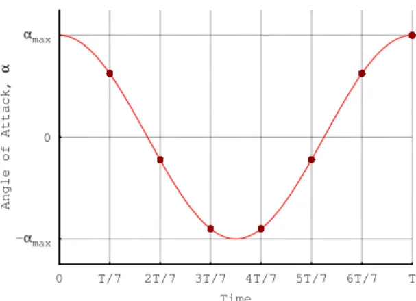
levels within one period of motion. For example, the airfoil locations at each of the sub-time levels of a three harmonic calculation are shown for a simple pitching airfoil in Fig. 3.1. These sampled values can then be assembled into vector form as given by Eq. 3.10. Ql,j = Ql,j(t0+ ∆t) Ql,j(t0+ 2∆t) .. . Ql,j(t0 +T) , Nl,j = Nl,j(t0+ ∆t) Nl,j(t0+ 2∆t) .. . Nl,j(t0 +T) (3.10) T = 2π ω ∆t= 2π NTω
The Fourier coefficients of the conservation variable (Qˆl,j) can be related to the
time-domain conservation variables sampled over one period (Ql,j) by the NT ×NT
discrete Fourier transform matrix [E] and likewise for the spatial operator.
ˆ Ql,j = [E]Ql,j, Nˆl,j = [E]Nl,j (3.11) E = 2 NT 1/2 1/2 . . . 1/2 cos(2πN1×1 T ) cos( 2π1×2 NT ) . . . cos( 2π1×NT NT ) .. . cos(2πNT×1 NT ) cos( 2πNT×2 NT ) . . . cos( 2πNT×NT NT ) sin(2πN1×1 T ) sin( 2π1×2 NT ) . . . sin( 2π1×NT NT ) .. . sin(2πNT×1 NT ) sin( 2πNT×2 NT ) . . . sin( 2πNT×NT NT ) (3.12)
With this substitution, Eq. 3.8 can be expressed in terms Ql,j and Nl,j as given
below.
-αmax 0 αmax 0 T/7 2T/7 3T/7 4T/7 5T/7 6T/7 T Angle of Attack, α Time
(a) Angle of attack at each sub-time level.
(b) Airfoil location for each sub-time level.
Figure 3.1: Airfoil location at each sub-time level of a three harmonic calculation.
Multiplying by the inverse of [E] results in
ω[D]Ql,j−Nl,j =0 (3.14)
where [D] = [E]−1[A][E].
Equation 3.14 represents the governing equations recast in the frequency-domain. There are several important features of this equation. First, note that the first term in the above equation is a pseudo-spectral (frequency-domain) representation of the time derivative term. This term is referred to as the source term of the equation since it contains no time derivatives per se. The second important feature of this
equation is that the spatial operator is unchanged from the time-domain formulation, it is simply evaluated at multiple sub-time levels. This is critical to the goal of implementing the HB method about an existing time-domain solver. Finally, note that the vector equation for each conservation variable at each point is of size NT.
In order to mimic the form of the time-domain equations as closely as possible, a pseudo-time (non-physical time) term is added to Eq. 3.14. The result is an equation that is identical in form to Eq. 3.2 with one extra term, i.e. the source term.
∂Ql,j(t)
∂τ −Nl,j(t) +ω[D]Ql,j(t) = 0 (3.15)
Since the frequency-domain representation of the governing equations is given by Eq. 3.14, the pseudo-time term can be used to iterate rapidly to convergence. Equation 3.15 can be discretized in pseudo-time using the same methods by which the original time-domain equations are discretized in physical time. Also, recall that the spatial operator is unchanged from the time-domain solver. This results in a finite-difference formulation of the HB method that is formally unchanged from that of the original time-domain CFD code except for the addition of the source term.
3.2
Stability Analysis
As with time-domain equations, the choices made when discretizing Eq. 3.15 affect the numerical stability of the scheme. Additionally, there is a choice to be made regarding the inclusion of the source term; it can be included on the n pseudo-time level or the n+ 1 pseudo-time level. As will be shown in the following sections, each of these options have serious limitations.
The 1-D advection equation, as given by Eq. 3.16, will be used to analyze potential discretization techniques.
∂Q ∂t +c
∂Q
As to be expected, it will be shown that the numerical stability of the frequency-domain representation of Eq. 3.16 depends on the type of discretization used. It will also be shown that the discretization of the source term greatly influences the stability of the scheme and the size of the system of equations that must be solved. When recast in the frequency-domain, the advection equation becomes the following.
∂Q ∂τ +c[I]
∂Q
∂x +ω[D]Q= 0 (3.17)
In the following sections we will analyze including the source term on the n pseudo-time level and then+ 1 pseudo-time level. For each of these options we will analyze the stability of the Euler implicit and explicit backward difference methods applied to Eq. 3.17.
3.2.1 Source Term Included in the n Pseudo-time Level
Consider the matrix system associated with the time-domain version of the advection equation (Eq. 3.16.) The discretization of this equation (or any PDE) can be formed into a Nnodes×Nnodes system of equations given by Eq. 3.18.
[A]∆Q= [B]Qn (3.18)
Recall that the harmonic balance method requires solving a system of equations of sizeNT for each conservation variable at each node. Thus, for a scalar equation being
solved on a domain of sizeNnodes, the HB linear system would take the following form
where ˆQis of size NT ·Nnodes.
[A]∆ ˆQ= [B] ˆQn+ω[D]Q (3.19)
The vector containing the value of Q at each node on each sub-time level can be constructed as shown in Eq. 3.20 whereQ1, for example, represents vector containing
the solution at each node of the first sub-time level. Q= Q1 Q2 .. . Q3 (3.20)
For clarity we will analyze the form of the HB system of equations considering only one harmonic, as one harmonic is sufficient to demonstrate the features of the system. When the source term of the HB method is included on the n pseudo-time level, the system takes the following form
[A] [A] [A] ∆Q1 ∆Q2 ∆Q3 = [B] [B] [B] Q1 Q2 Q3 n + s1 s2 s3 (3.21)
where the source term is given by Eq. 3.22.
s1 s2 s3 =ω D Q1 Q2 Q3 n (3.22)
The source term matrix D is a full matrix of size Nnodes·NT ×Nnodes ·NT, which
couples the sub-time levels. However, since this is evaluated on thentime-level it can be computed before the update takes place. The result is that this large linear system does not need to be constructed. Instead, the update for each sub-time level (each row in the above equation) can be calculated independently of the others. This is highly favorable since it would be very costly to solve this fullNnodes·NT×Nnodes·NT linear
system. Also, note that the update for the frequency-domain system of equations is unchanged from the time-domain version for each sub-time level with the exception of the source term. With such similarity to the time-domain update, little must be changed when converting a time-domain solver to the HB method.
Stability of the Backward Difference Discretization
Applying the simple backward difference discretization to Eq. 3.17 and including the source term on the n pseudo-time level results in
Qn+1 j −Q n j +λ Q n j −Q n j−1 +ω[D]Qn j =0 (3.23)
where λ=c∆τ /∆x. Note that [D] is a circulant matrix, which can be decomposed into [P][L][P]−1 where the columns of [P] are the Eigenvectors of [D], and [L] is the diagonal matrix containing the Eigenvalues of [D] as given below wherei=√−1.
[L] =i −NH . .. 0 . .. NH (3.24)
Premultiplying Eq. 3.23 by [P]−1 results in a diagonal system of equations where each row is identical except for the coefficient multiplying the source term. Thus, the stability of the method can be determined by analyzing one scalar equation as given in Eq. 3.25.
qnj+1−qnj +λ qnj −qnj−1+miω∆τ qjn= 0 (3.25) m∈[−NH, NH]
By performing a von Neumann stability analysis of Eq. 3.25, we find that the amplification factor associated with the method is given by
r= 1 +λ(cosβ−1−isinβ)−imω∆�
![Figure 4.1: Development history of OVERFLOW 2. Figure adapted from OVER- OVER-FLOW 2.1 Manual [1].](https://thumb-us.123doks.com/thumbv2/123dok_us/29987.2504159/68.918.190.785.115.869/figure-development-history-overflow-figure-adapted-flow-manual.webp)