Bayesian Estimation of a Dynamic
Partial-Equilibrium Model for Investment
∗
Matthias Kredler
†August 26, 2005
Abstract
This paper revisits the question if the user cost of capital plays an important role for investment decisions using Bayesian estimation techniques. These methods offer advantages over classical econometric tools in this area: The most important are that prior distributions offer a convincing way to confine the support of model parameters and that confidence intervals are more reliable when model parameters approach the bounds of their support. I use aggregate investment data from six industrial sectors in the UK to estimate a parsimonious partial-equilibrium model. The Kalman Filter is used to evaluate the likelihood and MCMC methods are employed to draw from the posterior distribution. The main finding is that the real interest rate accounts for less than 10 percent of the variance in investment under the 99-percent confidence level; this result is robust across sectors.
∗This paper is handed in as a term paper for the course “Advanced Macroeconomics”,
taught by T. Sargent and F. Schorfheide atNew York Universityin the Fall 2004 semester.
1
Introduction
Surprisingly, it is still an open question in macroeconomics if the user cost of capital matters for investment. On a theoretical level, all standard models predict that the real interest rate should have a major impact on investment.1
On an empirical level, however, this effect is hard to find. As Caballero (2000) notes, “the empirical investment literature has been nearly merciless in evaluating [these] theories”. He summarizes the empirical literature by saying that even studies thatdo find an impact of the user cost of capital on investment leave a large fraction of the variance in investment unexplained.
In the last two decades, yet, evidence has accumulated that the impact of capital costs on investment is larger than previously thought. Caballero (2000) cites studies that focus on long-run capital formation and episodes where investment incentives underwent changes due to tax reform; in all of these studies, the coefficients on the cost of capital are larger than in previous work. Bernanke (1983) found that high real interest rates were largely responsible for the low pace of capital expenditure in the late 1970s and early 1980s in the U.S.
Recently, new methods have been added to the econometrician’s toolkit that warrant a new look at this topic: The vast increase in computing power and the development of Markov-Chain Monte-Carlo (MCMC) methods have made the estimation of Bayesian models feasible on standard personal com-puters. These techniques offer some significant advantages over frequentist methods.
First, they give the researcher the possibility to force certain model pa-rameters into the economically sensible range by specifying their prior distri-bution. Moreover, as Johannes & Polson (2005) note, they offer a coherent treatment of both model parameters and hidden state variables in the model — they treat both as random variables which have a joint distribution with the observables. In many cases, also, Bayesian methods are more reliable and robust than classical maximization-based methods; this is especially the case when filtering methods are employed to evaluate the likelihood of an ob-served time series. Ill-behaved likelihood surfaces and the lack of analytical derivatives can make maximization in a high-dimensional parameter space a formidable task.
Lastly, and maybe most importantly, the Bayesian approach yields exact
confidence intervals for the parameters as well as for functions of these; in our case, for example, the fraction of variance in investment explained by movements in the interest rate. If this fraction is close to zero, the Bayesian approach yields confidence intervals that are much more credible than the ones obtained from first-order approximations in a classical framework. The latter are bound to be symmetric and will extend below zero in many cases although they refer to a fraction, which by definition has to be positive.
In this paper, I estimate a parsimonious partial-equilibrium model for ag-gregate investment in six industrial sectors in the UK with Bayesian methods. I use the Kalman Filter to evaluate the likelihood and draw from the poste-rior distribution of the parameters and the hidden state of the model using MCMC methods. The main finding is that the real interest rate accounts for less than 10 percent of the variance in investment in all of these sectors; this statement holds under a 95-percent confidence level. However, as in prob-ably any model, there are indications of misspecification which suggest to compare this parsimonious framework to different, possibly more elaborate, models in future research.
2
Data
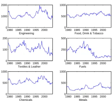
The data set for investment is taken from the UK’sOffice for National Statis-tics’s web site. It consists of six quarterly time series for aggregate business investment by industry at 2001 prices in millions of British Pounds. The six industries are: Chemicals; Engineering; Food, Drink & Tobacco; Fuels; Met-als; Textiles & Leather. The data set ranges from the first quarter of 1979 to the fourth quarter of 2004, yielding 104 observations. The time series are seasonally adjusted and measure investment by total capital expenditure in the sector. The time series are plotted in figure 1.
As for the cost of capital, it would be optimal to use some direct measure of the real interest rate in the estimation. Inflation-indexed bonds traded on the British capital markets come very close to such a direct measurement. However, these instruments are only traded at very long maturities. Also, as Barr & Campbell (1996) note, these bonds are only imperfect measures of real interest rates — even in the long term — since they leave the buyer unprotected against inflation occurring in the last months before maturity. Instead, I choose to use the ex-post real interest rate and regard it as a noisy signal of the expected real interest rate in the market. This procedure uses
Figure 1: Investment Data 1980 1985 1990 1995 2000 0 1000 2000 Engineering 1980 1985 1990 1995 2000 0 500 1000
Food, Drink & Tobacco
1980 1985 1990 1995 2000 0
100 200
Textiles & Leather
1980 1985 1990 1995 2000 0 250 500 Fuels 1980 1985 1990 1995 2000 0 500 1000 Chemicals 1980 1985 1990 1995 2000 0 500 1000 Metals
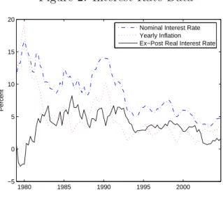
the Kalman Filter and is due to Fama & Gibbons (1982). The ex-post real interest rate is defined as the difference between the nominal interest rate and inflation. The data are taken from the Bank of England’s web site. Figure 2 shows the respective time series over the sample period.
For inflation, I take the difference between the logarithm of the price level over one year.2 Hamilton (1994b) suggests this as a simple procedure
to remove seasonality. Technically, the resulting figure is a 4-quarter moving average over annualized quarterly inflation (seasonally adjusted) andnot an-nualized quarterly inflation. Yet, this smoothing of the inflation time series essentially removes noise from the data and should not have a significant effect on the results — the relevant variable in the estimation procedure is the underlying expected inflation (in seasonally adjusted terms), which has certainly less variance in the high frequencies than realized inflation.
Visual inspection suggests that the series can be assumed to be stationary over the sample period. Hence, no effort will be made to include a time trend in the theoretical model.
2
Technically: πt= logCP It+4−logCP It, where πt is annualized inflation in quarter
Figure 2: Interest-Rate Data 1980 1985 1990 1995 2000 −5 0 5 10 15 20 Percent
Nominal Interest Rate Yearly Inflation Ex−Post Real Interest Rate
3
The Model
The model describes a dynamic partial equilibrium in a competitive industrial sector, where the interest rate and demand are exogenous. The representative firm in the sector produces a single good with a constant-returns-to-scale technology. The only factor employed is capital:
yt =Akt,
where yt is the quantity of the good produced by the firm in period t, kt is
the capital stock in t, and A > 0 is a productivity coefficient. I use lower-case letters to denote quantities on the firm level and capitals to denote their aggregate analogon. Capital accumulation is frictionless:
kt+1 = (1−δ)kt+it, (1)
whereitis investment by the firm in periodtand 0≤δ ≤1 is the depreciation
rate. The investment good it can be obtained at the constant price of one
unit of the output good. Demand for the good produced in the sector is given by
Pt =CdYt−γνt=CdA−γKt−γνt, (2)
where Pt is the price of the good,Cd>0 is a sector-specific constant, andYt
and time-invariant. The demand shifter νt induces time-varying investment
incentives in the sector; its logarithm ˜νt ≡ logνt is assumed to follow an
AR(1) process with a Gaussian innovation:
˜
νt+1 =ρνν˜t+σνε˜ν,t+1, (3)
where ˜εν
t is a serially uncorrelated normal shock with variance 1. To simplify
notation, introduce C ≡CdA−γ >0.
Notice that technology shocks can easily be accommodated in this frame-work. Suppose we introduce an adequately scaled process ξt for the
produc-tivity of capital: yt =Aktξt. Then, equation (2) becomes: Pt=CKt−γνtξ−tγ.
In this alternative framework, ˆνt≡νtξt−γ would be the demand shifter.
Un-fortunately, I did not find data series that allow me to disentangle the effects of demand and technology. This would be an interesting extension of this project.
The firm is risk-neutral and has access to an incomplete capital market. There is an exogenously given stochastic sequence for the real interest rate
Rt. Specifically, I assume that its deviation from the logarithmic mean,
˜
rt ≡ logRt− E[logRt], follows an AR(1) process with a standard normal
serially uncorrelated shock:
˜
rt+1 =ρrr˜t+σrε˜r,t+1 (4)
The following notation is adopted to facilitate the ensuing discussion:
R−10,t =
t−1
Y i=0
Ri−1,
The firm ranks stochastic sequences of profits by the criterion
Q {kt+1}∞t=0,· =E0 ∞ X t=0 R−10,t CKt−γνtkt−kt+1+ (1−δ)kt given k0,{Kt+1}t∞=0,{Rt}∞t=0,
where the sequences{Kt+1}∞t=0,{Rt}∞t=0are exogenous and the sequence{kt+1}∞t=0
is under control of the firm. The term in brackets is the firm’s profit in pe-riod t, which consists of the revenue from sales and the cost of investing in the capital stock.
Taking first-order conditions with respect to kt+1 and re-arranging yields
the following familiar expression:
Rt =CKt−+1γEt[νt+1] + (1−δ) (5)
This equation says that the expected profits from investing a marginal unit in a company in the sector must be equal to the interest rate on the capital market. Notice that no variable under control of the firm enters in (5). The equation only gives a restriction on aggregate quantities which makes a risk-neutral investor indifferent between investing a marginal unit in the sector or holding a bond in the wider capital market. In order to obtain a tractable linear expression, I take a first-order Taylor approximation of (5) in logarithms and re-arrange to obtain3
˜ kt+1 = ρν γ ν˜t− ¯ R γ[ ¯R−(1−δ)]r˜t, (6) where ˜kt ≡ logKt−E[logKt] and ¯R ≡ E[logKt]. Using equations (3), (4)
and the expectation of (6), the impulse response for capital with respect to the driving processes is
˜ kt+1 = ρνσν γ ∞ X j=0 ρjνε˜ν,t−j − ¯ Rσr γ[ ¯R−(1−δ)] ∞ X j=0 ρjrε˜r,t−j. (7)
To obtain an expression for investment, use the log-linearized law of mo-tion of capital, ˜kt+1 = (1−δ)˜kt+δ˜it: ˜it = ρνσν γ 1 δε˜ν,t+ ∞ X j=1 ρjνε˜ν,t−j ! − Rσ¯ r γ[ ¯R−(1−δ)] 1 δε˜r,t+ ∞ X j=1 ρjrε˜r,t−j ! (8) The variance of investment can be decomposed as
V ar(˜it) = ρνσν γ 2 1 δ + ρ2 ν 1−ρ2 ν − ¯ Rσr γ[ ¯R−(1−δ)] 2 1 δ + ρ2 r 1−ρ2 r .
The second observed variable is the ex-post real interest raterp,t, which is
defined asrn,t−πt, where rn,t is the nominal interest rate and πt is inflation. 3Note that when taking expectations of this first-order approximation (or equivalently, in the so-called “deterministic steady state”), the following identity follows: ¯R−(1−δ) =
The ex-ante real interest rate rt is defined as rn,t −πe,t, where πe,t is the
inflation rate expected for period t by the public when entering this period. I follow Fama & Gibbons (1982) and decompose realized inflation into πt=
πe,t+ηt, where ηt is a rational-expectations error. Regarding rt as a hidden
state and combining the expressions before, we have
rp,t=ri,t−πt=rt−ηt. (9)
Since ηt is a rational-expectations error, it is uncorrelated over time and also
uncorrelated to other variables known to the agents in the market at time t, as for example the contemporaneous shocks εν,t+1 and εr,t+1. I furthermore
assume that ηt has constant variance ση.
Now, everything is in place to write down a state-space system combining (3), (4), (8) and (9): ˜ νt+1 ˜ rt+1 ˜ k0 = ρν 0 0 0 ρr 0 0 0 1 ˜ νt ˜ rt ˜ k0 + σν 0 0 σr 0 0 ˜ εν,t ˜ εr,t (10) ˜ it ˜ rp,t = −Ptj=1(1−δ)jLj 0 ˜it+ ρδγν −R¯ δγ[ ¯R−(1−δ)] − (1−δ)t δ 0 1 0 ! ˜ νt ˜ rt ˜ k0 + 0 ση ηt,
where (˜ε′ν,t+1,ε˜r,t′ +1, η′t)′ is Gaussian white noise with covariance matrix I 3
and Lis the lag operator: Lxt =xt−1. In the language of the Kalman Filter,
(˜νt,r˜t,k˜0)′ is the hidden state and (˜it,r˜p,t)′ is the observed state. The lagged
values of ˜it are pre-determined at t and can hence be treated as fixed. The
timing convention is as follows: The first observation is made at t = 1, the last at t=T.
The distribution of the hidden state att = 0, which is needed to start the recursions of the Kalman Filter, is the unconditional variance of the variables. From (8), the unconditional variance of ˜k0 can be seen to be
V ar(˜kt+1) = ρν γ 2 V ar(˜νt) + ¯ R γ[ ¯R−(1−δ)] 2 V ar(˜rt), where V ar(˜νt) = σ 2 ν 1−ρ2 ν and V ar(˜rt) = σ2 r 1−ρ2
and ˜rt are
Cov(˜kt+1,ν˜t+1) = Cov(˜kt+1, ρνν˜t) +Cov(˜kt+1, σνε˜ν,t+1) =
ρ2
ν
γ V ar(˜νt) Cov(˜kt+1,r˜t+1) = Cov(˜kt+1, ρr˜rt) +Cov(˜kt+1, σrε˜r,t+1) =
ρrR¯
γ[ ¯R−(1−δ)]V ar(˜rt)
4
Estimation and Computational Issues
I adopt a two-stage strategy to estimate the model described in (10). In the first stage, the parameters ρν, σν and ση are determined solely from the
interest-rate data by maximum-likelihood estimation (MLE). In the second stage, these parameters are fixed at the estimated values and the remaining four parameters in (10) are estimated from the investment data in a particular sector and the interest-rate data employing Bayesian methods.
This two-stage strategy is not only computationally easier to implement than joint estimation of all seven parameters. It is also in another way a natural way to proceed. Since the six investment time series from the differ-ent sectors all contain a noisy signal about the real interest rate that adds to the information contained in the ex-post real rate, it would be theoreti-cally appealing to estimate a model with all sectors jointly. However, this is obviously hard to implement. The alternative strategy of estimating the seven parameters in (10) jointly ineach of the six sectors, on the other hand, is somewhat awkward as well, since all estimation procedures would yield slightly different posterior distributions for the time path of the real rate. Therefore, the two-stage strategy seems a reasonable way to proceed. At any rate, potential inefficiencies of this method should be small since the invest-ment time series can be expected to contain very little additional information on the real interest rate.
The first step evaluates the likelihood of observing the data for{r˜p,t}104t=1
for a fixed triplet of parameters (ρν, σν, ση)′ by applying the Kalman Filter
to the simplified system4
˜
rt+1 =ρν˜rt+σνεν,t
˜
rp,t= ˜rt+σηηt.
4See Hamilton (1994a), for example, for the exact procedure of obtaining the likelihood in a state-space system.
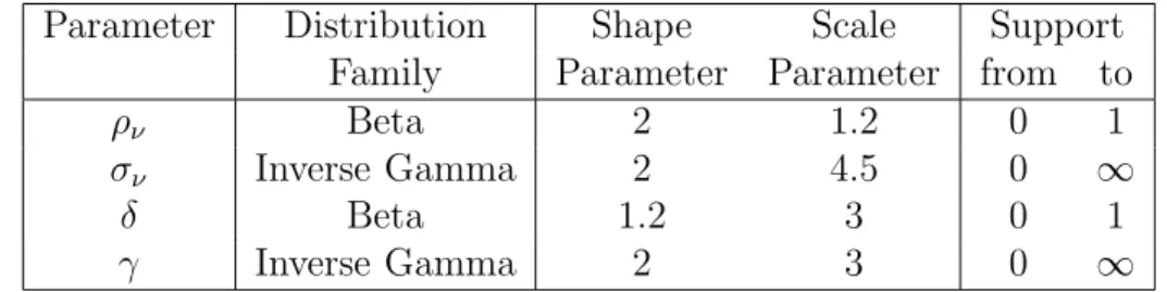
Table 1: Prior Distribution
Parameter Distribution Shape Scale Support Family Parameter Parameter from to
ρν Beta 2 1.2 0 1
σν Inverse Gamma 2 4.5 0 ∞
δ Beta 1.2 3 0 1
γ Inverse Gamma 2 3 0 ∞
The series {˜rp,t}104t=1 is obtained by de-meaning the logarithm of the ex-post
real interest rate, as described in section 2. Notice that this procedure yields a method-of-moments estimate for the parameter ¯R, which will be used in the second step as well.
As in all subsequent estimation procedures, I calculate the matrices aris-ing in the application of the Kalman Filter dynamically until they converge to the stationary steady state. These steady-state matrices are computed us-ing the doublus-ing algorithm5. This proved to be important since the matrices
in the dynamic algorithm diverged after a large number of periods, probably due to small calculation inaccuracies accumulating over time.
In the second stage, the Metropolis-Hastings algorithm6 is used to draw
from the posterior distribution of the remaining four parameters ρν, σν, δ
and γ. The prior distribution of the parameters is given in table 4. The four parameters are independently distributed under the prior.
The likelihood of observing the data {r˜p,t,˜it}104t=1 given a vector of
pa-rameters is evaluated applying the Kalman Filter to the state-space system described in (10). To obtain the series{˜it}104
t=1, again I de-mean the logarithm
of the investment time series in the respective sector, which is tantamount to estimating the model parameter C by a moment condition.
Since (10) contains a dynamic component, it is necessary to work with a time-varying system for a certain number of periods. For small values ofδ, the matrices calculated for the Kalman Filter do not converge for a long time and sometimes the time-varying system has to be used until the end of the data series. In the other cases, the matrices from the doubling algorithm of the limiting system are utilized after a number of periods applying a convergence
5Specifically, I use a program that Ljungqvist & Sargent (2004) provide.
6See Johannes & Polson (2005), for example, for a description of how to MCMC tech-niques.
criterion. For this stable system, the component ˜k0 is dropped from the
hidden state.
As suggested by Johannes & Polson (2005), a fat-tailed distribution is used for the jump proposals in the Metropolis-Hastings algorithm. Specif-ically, I use a t-distribution with 5 degrees of freedom. In the estimations, it proved very important to adjust the scaling of the jump-proposal density to the covariance of the parameters under the posterior. As figure 8 in the appendix suggests, especially the covariance between the parameters γ and
σν is very high; in all sectors, their correlation coefficient under the
poste-rior distribution exceeds 0.9. Implementing a well-scaled proposal density allowed me to increase the efficiency of the algorithm by using a relatively large variance for the jump proposals. The jump size was tuned such that the acceptance rate lay in the optimal range between 0.25 and 0.4.7
The computations were carried out inMatlab and were greatly simplified by the use of object-oriented programming to calculate the likelihood under different parameter vectors and for different dimensions of the hidden state vector.8
For each sector, I carried out 20,000 draws from the posterior distribution. For every tenth draw, an additional draw was taken from the process for the hidden state in (10). This strategy is due to the high computational demands of carrying out these draws — note that drawing from this process requires both more memory usage and additional computations to those of the Kalman Filter.
The technique I use to draw from the hidden state is inspired by the smoothing algorithm as described, for example, in Hamilton (1994a).9 To
simplify notation, denote a generic state-space system (as the one in (10)) as
7See Johannes & Polson (2005) for an overview of theoretical results on the optimal acceptance rate of MCMC algorithms.
8Recall that the initial capital stock is dropped from the system once convergence is reached and so the number of hidden states decreases from three to two.
9“Smoothing” describes a recursive procedure for obtaining the conditional expectation (or projection, in the non-Gaussian case)E[xt|yT] with its associated conditional variance (or mean squared error). Note that the Kalman Filter only gives a recursive formula for findingE[xt|yt] andE[xt+1|yt] — it does not take into account future observations ofyt, which potentially contain useful information about the distribution ofxt.
follows:
xt+1 =Axt+Cεt yt=Fxt+Gηt,
where xt is a vector of hidden state variables, yt is a vector of observed
variables, (ε′t,η′t)′ is vector white noise and the matricesA,C,Fand G are
known at t and fulfill the obvious conformability conditions with the state and shock vectors. Note that the following derivation is valid for time-varying matrices At, Ct, Ft and Gt as long as they are known at t — the subscript
is dropped for notational convenience only.
The following identity is at the heart of the algorithm:
E[xt|xt+1,yT] =E[xt|xt+1,yt],
where yt ≡ (y0,y1, . . . ,yt). This can easily be seen by decomposing yt+j
into yt+j =F " Aj−1xt+1+ j−1 X k=0 AkCεt+j−k # +Gηt+j
and noting that the errors εt+k and ηt+k are uncorrelated with xt for k >0
by assumption. To facilitate notation, introduce ˆxt|t ≡ E[xt|yt], ˆx
t+1|t ≡
E[xt+1|yt] and ˆxdt ≡ E[xt|xt+1,yt], where the d in the superscript indicates
that this value will be used for drawing from the posterior. Now, update the projection ofxt on yt, which is a by-product of the Kalman Filter, with the
information about xt+1. Make the “news” from xt+1 orthogonal on yt by
introducing the innovation at+1 ≡xt+1−xˆt+1|t and update using the formula
for updating a linear projection (as given in Hamilton (1994b), for example):
ˆ xdt =E[xt|xt+1,yt] = ˆxt|t+E h (xt−xˆt|t)a′t+1 i | {z } ≡Ωxa n E[at+1a′t+1] | {z } ≡Ωt+1|t o−1 at+1 (11)
Notice that Ωt+1|t is also an ingredient of the Kalman Filter and hence does not require additional computations. As for Ωxa, it is given by
Ωxa =E h (xt−xˆt|t)a′t+1 i =Eh(xt−ˆxt|t) A(xt−xˆt|t) +Cεt+1 ′i =Ωt|tA′,
where Ωt|t ≡ E[(xt−xˆt|t)(xt−xˆt|t)′] is again an ingredient of the Kalman
The variance of the true state xt around E[xt|xt+1,yt] is given by the
usual formula for the mean squared error of an updated linear projection:
Ωtd≡E[(xt−xˆdt)(xt−xˆdt)′] =Ωt|t−ΩxaΩ−1t+1|tΩxa (12)
Since the variables{yt,xt}Tt=1are by assumption jointly normally distributed,
the conditional varianceE[(xt−xˆdt)(xt−xˆdt)′|xt+1,yt] is equal to the variance
Ωd
t which is unconditional on (xt+1,yt).
The algorithm to draw a sequence {xt}T
t=1 from its distribution
condi-tional on a sequence {yt}Tt=1 is as follows:
• Initialize by setting t:=T, ˆxdt = ˆxT|T and Ωdt =ΩT|T, which can both
be obtained from the Kalman Filter.10
• Draw xt= ˆxdt +
Ωdt1/2χt, where χt ∼ N(0,I).
• Set t := t−1. Stop if t = 0 is reached. If not, update ˆxdt according to (11) and Ωdt according to to (12).
5
Results
The results of this first step are summarized in table 2. Figure 3 shows the filtered series (i.e. E[rt|rp,t, rp,t−1, . . .]) with confidence intervals, derived
from the conditional variance of the true statertaround its conditional mean
E[rt|rp,t, . . .].
Table 2: Results of 1st-stage Estimation (MLE) Parameter ρν σν ση
Estimate 0.95 1.2 0.35
In the second step, the MCMC estimation yielded very similar results across the six sectors. Table 3 shows posterior mean and variance for the
10
There were some computational difficulties involved in this step since the updated matrices lost the property of positive definiteness for some parameter draws. These irreg-ularities occurred very rarely and were obviously due to computational inaccuracies when the vectors in Ωd
t were close to collinear. The problem was fixed by adding very small numbers to the elements of the matrix to make it positive definite whenever this property was lost.
Figure 3: Results of 1st-stage Estimation: Filtered Series for rt 1980 1985 1990 1995 2000 −6 −4 −2 0 2 4 6
Percent−deviation of real interest rate from mean
Filtered Series 95% Confi− dence Bands. Data
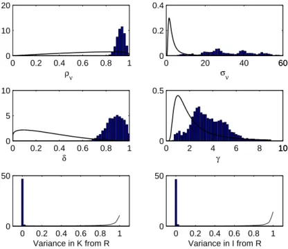
model parameters and ˜k0. Figure 4 shows the marginal distribution of the
parameters and the proportion of variance in capital and investment caused by interest-rate movements under the posterior for the sector Engineering. The black curves describe the distribution of the respective parameter under the prior11 — it is easy to see that the priors are not very restrictive and
have little influence on the posterior.
There are two features of the results that are unexpected: First, the rather high estimates for the depreciation rate δ are surprising. They suggest that more than 80 percent of the capital stock are obliterated every quarter in the
Chemicals sector, for example, if the underlying story of the model is taken
seriously. This result hints at a misspecification issue here and suggests to test other specifications for the investment process, e.g. specifying some form
11For the two bottom panels, which describe complicated functions of the deep model parameters, the calculation of the prior density is a non-trivial task — using the theorem on the transformation of probability densities, it would be possible to obtain the densi-ties of these random variables in closed form. Since this would involve integration over several complicated functions, I opted for a simulation method. A very large number of draws (1,000,000) was taken from the independent distributions of the deep model param-eters and the respective function values were calculated . Then, a simple histogram was obtained.
Figure 4: Posterior Distribution for the Sector Engineering 0 0.2 0.4 0.6 0.8 1 0 10 20 ρν 0 20 40 6060 0 0.2 0.4 σν 0 0.2 0.4 0.6 0.8 1 0 5 10 δ 0 2 4 6 8 101010 0 0.5 γ 0 0.2 0.4 0.6 0.8 1 0 50 Variance in K from R 0 0.2 0.4 0.6 0.8 1 0 50 Variance in I from R
Table 3: Posterior Mean and Standard Deviation
Sector ρν σν δ γ ˜k0
Engineering 0.926 31.845 0.876 3.619 0.253
0.033 12.01 0.072 1.479 9.8
Food, Drink & Tobacco 0.916 46.891 0.667 10.245 0.047
0.035 21.159 0.076 4.702 6.129
Textiles & Leather 0.927 13.91 0.766 1.1 0.247
0.039 8.39 0.111 0.716 26.399 Fuels 0.974 24.275 0.608 2.28 -0.09 0.014 7.456 0.086 0.805 18.095 Chemicals 0.903 32.671 0.841 4.128 0.249 0.04 14.65 0.085 1.951 8.988 Metals 0.928 16.758 0.895 1.647 0.558 0.03 13.047 0.067 1.309 24.983
(Means are given above in normal script size, standard deviations below in footnote size.)
of adjustment cost or lumpiness in investment.
Second, the high variability of the model parametersσν andγ paired with
their large covariance could be an indicator for problems with identification in this model. As described in the appendix B, however, this problem does not arise with simulated data where interest rates have a significant impact upon investment — note that this is not the case for either of the data series in the estimation. In fact, the following results on the importance of the interest rate for investment are not affected by the “misbehavior” of the deep model parameters.
The most striking result of the estimations is the very low fraction of variance accounted for by the interest rate — see table 4 for some percentiles of this statistic across the different sectors. Its mean is below 2.5 percent in all sectors, and only in one sector does the 99th percentile exceed 10 percent.
The impulse responses of investment to a one-standard-deviation shock to the demand shifter and the real interest rate are given in figure 5. The solid line depicts the mean of the analytical impulse response as given in (7) and (8) under the posterior; the dotted lines are 95-percent confidence intervals.
Table 4: Proportion of Variance in Investment due to Interest Rate Sector Mean 95th Percentile 99th Percentile Engineering 0.0024 0.0081 0.0218 Food, Drink & Tobacco 0.0061 0.0371 0.0739 Textiles & Leather 0.0211 0.0714 0.1068 Fuels 0.0025 0.0096 0.0190 Chemicals 0.0041 0.0162 0.0318 Metals 0.0161 0.0627 0.0987
Figure 5: Impulse Responses for the SectorEngineering
0 5 10 15 20 0
0.5 1
Impulse Response for Capital Stock
Shock to Demand
0 5 10 15 20 −1
−0.5 0
Shock to Interest Rate
0 5 10 15 20 0
0.5 1
Impulse Response for Investment
0 5 10 15 20 −1
−0.5 0
are depicted in figure 6. Note that these distributions mirror both the un-certainty about the deep model parameters remaining after the estimation and the uncertainty about the hidden state that remains after any filtering exercise. For this reason, the size of the confidence intervals is time-varying, which may be striking at first for the reader accustomed to the constant conditional variances that characterize the Kalman filter under parameter certainty. It is important to bear in mind the additional dimension of pa-rameter uncertainty that arises in a Bayesian estimation framework.
Figure 6: The Demand Shifter νt
1980 1985 1990 1995 2000 −400 −200 0 200 400 Engineering 1980 1985 1990 1995 2000 −400 −200 0 200 400
Food, Drink & Tobacco
1980 1985 1990 1995 2000 −400 −200 0 200 400
Textiles & Leather
1980 1985 1990 1995 2000 −400 −200 0 200 400 Fuels 1980 1985 1990 1995 2000 −400 −200 0 200 400 Chemicals 1980 1985 1990 1995 2000 −400 −200 0 200 400 Metals
Visual inspection suggests that the investment incentives faced by the firms in the different sectors are lowly correlated among each other. It seems that macroeconomic factors which affect all sectors and are not captured in interest rates (e.g. multi-purpose technologies, common components in demand, government policies) play a minor role in determining investment in the different sectors. Further econometric analysis of the joint properties of these processes or a model encompassing more than one sector would be an interesting extension of this exercise.
6
Conclusions
The estimations in this paper show that movements in the real interest rate accounted for very little variance in investment in six industrial sectors in the UK over the last 26 years. This statement can be made on a statisti-cally sound basis in a Bayesian estimation framework — I argue that confi-dence intervals derived from first-order approximations employed in frequen-tist stafrequen-tistics are inferior to the Bayesian concept of the posterior distribution when this fraction is very close to zero. Moreover, the Bayesian approach offers the possibility to force model parameters into the economically sensi-ble range and is very robust even when the dimensionality of the parameter space increases. All these are reasons to use econometric tool in the empirical evaluation of dynamic investment models.
Furthermore, the hidden investment incentives in the different sectors seem to have very little in common. This is surprising, since many macroe-conomic conditions other than the interest rate should have a similar impact on all sectors. An extension of this model to investigate this issue systemat-ically would be an interesting exercise.
Finally, one caveat is in place: The very high estimates for quarterly depreciation rates — in most sectors the posterior mean of this parameter is above 60 percent — suggest that the model employed in this paper is potentially misspecified. Future research could apply Bayesian methods to models with adjustment costs and irreversibilities in the investment process (as those of Abel & Eberly (1994) and Hayashi (1982)) or models that ac-knowledge the lumpiness of investment, a point that is emphasized by the empirical investment literature12. Another fascinating possibility is the the
use of particle filters or other non-linear methods, as described by Johannes & Polson (2005) and already used by Fern´andez-Villaverde & Rubio-Ram´ırez (2004), to explore the implications of theoretical models that going beyond first-order effects.
12
References
Abel, A. B. & Eberly, J. C. (1994), ‘A unified model of investment under uncertainty’, American Economic Review 84(5), 1369–1384.
Barr, D. G. & Campbell, J. Y. (1996), ‘Inflation, real interest rates, and the bond market: A study of UK nominal and index-linked government bond prices’, NBER Working Paper 5821 .
Bernanke, B. S. (1983), ‘The determinants of investment: Another look’,
American Economic Review73(2), 71–75. Papers and Proceedings of the
Ninety-Fifth Annual Meeting of the American Economic Association.
Caballero, R. J. (2000), ‘Aggregate investment: Lessons from the previous millenium’, Working Paper . AEA Session. In Memoriam: Robert Eis-ner.
Fama, E. F. & Gibbons, M. R. (1982), ‘Inflation, real returns, and capital investment’, Journal of Monetary Economics9(3), 297–323.
Fern´andez-Villaverde, J. & Rubio-Ram´ırez, J. F. (2004), ‘Estimating dy-namic equilibrium economies: Linear versus nonlinear likelihood’,
Jour-nal of Applied Econometrics . Forthcoming.
Hamilton, J. D. (1994a), State-space models, in R. Engle & D. McFadden, eds, ‘Handbook of Econometrics’, Vol. 4, Elsevier Science, Amsterdam: North Holland, chapter 50.
Hamilton, J. D. (1994b),Time Series Analysis, Princeton University Press.
Hayashi, F. (1982), ‘Tobin’s marginal q and average q: A neoclassical inter-pretation’, Econometrica 50(1), 213–224.
Johannes, M. & Polson, N. (2005), MCMC methods for continous-time finan-cial econometrics, in Y. Ait-Sahalia & L. P. Hansen, eds, ‘Handbook of Financial Econometrics’, Elsevier Science, Amsterdam: North Holland.
Ljungqvist, L. & Sargent, T. J. (2004), Recursive Macroeconomic Theory, 2 edn, MIT Press, Cambridge and London.
A
Parameter Paths in the MCMC Algorithm
Figures 7 and 8 show the path of the Markov chain for the four model param-eters in the estimation for theEngineering sector. For the parametersρν and
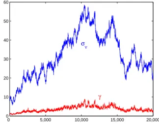
δ, the sensible range of parameter values is thoroughly explored — note that only 1,000 draws are shown in figure 7, whereas all 20,000 draws are shown in figure 8. For σν and γ, however, the picture is different — it would be quite
confident to assert that the chain has converged to a stationary distribution
for these two parameters.
Figure 7: MCMC Path of ρν and δ (SectorEngineering)
0 200 400 600 800 1,000 0.6 0.7 0.8 0.9 1 1 δ ρν
Due to their high correlation, the ratio betweenσν andγ stays in a
rela-tively stable range, so that other statistics of interest (as impulse responses and variance decompositions) do not vary much along the chain. The system described in (10) seems to come close to non-identifiability when the influence of interest rates on investment goes close to zero; yet, the main conclusion of the exercise — interest rates plays a minor role in determining investment — is very robust.
B
Estimation with Simulated Data
The data in this simulation were generated by drawing 104 independent stan-dard normal shock vectors (˜εν,t,ε˜r,t, ηt)′ and feeding them into the dynamic
Figure 8: MCMC Path of σν and γ (Sector Engineering) 0 5,000 10,000 15,000 20,000 0 10 20 30 40 50 60 σν γ
linearized system described in (10). The initial state was drawn from the sta-tionary distribution of the system. The parameters ρr, σr and ση were fixed
at the values obtained in the first estimation stage (described in sections 4 and 5). For the remaining parameters, the following values were chosen:
ρν = 0.9, σν = 2,δ = 0.1 and γ = 1.5. These true values are marked with a
black diamond in figure 9, which gives the results of an estimation that was carried out in exactly the same fashion as the estimation on the real data (described in section 4). The estimation procedure yields reasonable results. The posterior distribution does not depart far from the true values and the variance of the parameters under the posterior is modest. This indicates strongly that the model does not suffer from an identification problem.
Figure 9: Posterior Distribution in Simulation 0 0.2 0.4 0.6 0.8 1 0 5 10 ρν 1 2 3 4 0 1 2 σν 0 0.2 0.4 0.6 0.8 1 0 20 40 δ 1 2 3 0 2 4 γ 0 0.2 0.4 0.6 0.8 1 0 10 20 Variance in K from R 0 0.2 0.4 0.6 0.8 1 0 20 40 Variance in I from R