Price Development in the German Housing
Market
Thomas Mayer and Matthias Gehrke
Abstract Financial crises are often preceded by an asset market bubble or strong credit growth. To prevent further crises, it is essential to identify and combat excessive price and credit developments as early as possible. The momentum observed in the German housing market in recent years has led to concerns that a house price bubble already exists or still can emerge. However, a clear outcome is still missing. The present study analyses bubbles in the prices of owner-occupied flats in Germany by using the augmented Dickey-Fuller test and a generalized version of the sup augmented Dickey-Fuller test. A distinctive feature of the latter test is that it delivers a consistent date stamping strategy for the origination and termination of multiple bubbles. At first sight, there is evidence of so-called rational bubbles both in regional markets as well as in the overall German housing market. But most of them are linked to decreasing interest rates. Possibly, rational bubbles in seven German cities can be identified.
Thomas Mayer·Matthias Gehrke
FOM University of Applied Science Leimkugelstraße 6, 45141 Essen, Germany
[email protected] [email protected]
Archives of Data Science, Series A
(Online First) DOI 10.5445/KSP/1000085951/06
KIT Scientific Publishing ISSN 2363-9881
1 Introduction
The price development in Germany is currently discussed controversially in both media and empirical studies (e.g. BIS, 2016; Dombret, 2016; Deutsche Bundesbank, 2017; Empirica AG, 2017). As Tissot (2014) states a reasonable house price is a precondition of a stable economy as it has a great impact on the financial system as well as other parts of the economy. On the one hand, due to the rationing function, an overpriced housing market can lead to inefficient resource allocation and overcapacities as it was the case in Spain before the emergence of the global financial crisis (Dreger and Kholodilin, 2013). On the other hand, house prices are an important determinant of consumption. According to macroeconomic models and empirical studies, increased prices will lead to increased wealth and finally to increased consumption (Tissot, 2014). However, if there is a price bubble, the consumption may decrease disproportionately after the bursting of the bubble. Hence, according to Kivedal (2013) the negative consequences of decreased prices may be reinforced by a price bubble. An empirical study by Reinhart and Rogoff (2008) reveals that financial crises are often preceded by an asset market bubble or at least strong credit growth. Losses can easily spread to the whole economy if the asset price is driven by a high credit growth (Scherbina and Schlusche, 2012). This result was confirmed by the price development in the housing markets in industrial countries at the start of the 2000s (see Figure 4 in the appendix) and the emergence of the global financial crisis in 2007.
In contrast to the price development in other housing markets, German real house prices decreased until 2007, but have been increasing significantly, especially since 2009. In the light of the momentum in the German housing market and the potential consequences of unreasonably high prices, the German housing market must be closely monitored in order to detect price bubbles as early as possible. Although discussed controversially at various levels, the existence of a house price bubble could neither be clearly rejected nor clearly confirmed so far.
The present study aims at detecting house price bubbles on an aggregated level as well as in regional markets. The research of Kholodilin and Michelsen (2015) shows that, due to the regional segmentation of the housing market, it must be assumed that bubbles are visible in regional markets first. The data selected for the present study is in line with the data basis of other studies
concerning the house price development in Germany. Regional and aggregated data are considered. Yearly average purchase prices and rents of newly built and second-hand apartments for 127 German cities from 1990 to 2015 are provided by bulwiengesa AG (a German consulting firm and analyst in the segment of real estates). In addition to that price indices for condominiums and residential rents on aggregated level (2003/Q1–2016/Q3) as well as for 7 cities (1991–2015) published by the Verband deutscher Pfandbriefbanken (vdp, Association of German Pfandbrief Banks) are used. To show the existence or non-existence of bubbles, tests for stationarity and explosive behaviour are used.
2 German Housing Market
The characteristics of the German housing market in 1990–2016 can be described by four key facts:
1. Converse price development:
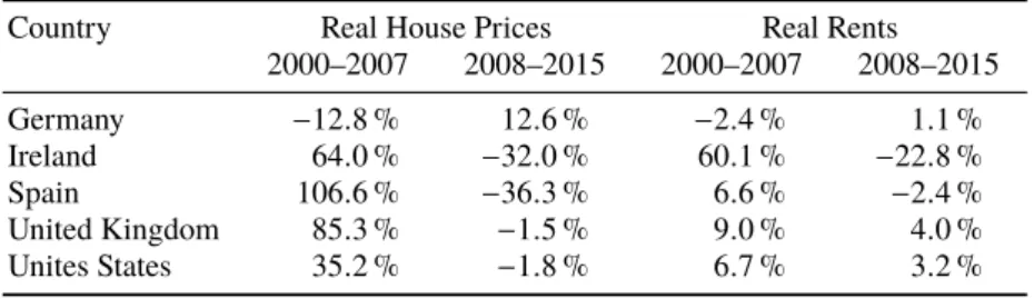
As indicated in Section 1, real house prices as well as rents are currently increasing after a long period of declining or stagnating prices and rents which can be traced back to the German reunification boom in the early 1990s (Michelsen and Weiß, 2009). This is in contrast to the price development in other industrial countries as illustrated in Table 1.
Table 1:Development of real house prices and rents in selected countriesa.
Country Real House Prices Real Rents
2000–2007 2008–2015 2000–2007 2008–2015 Germany −12.8 % 12.6 % −2.4 % 1.1 % Ireland 64.0 % −32.0 % 60.1 % −22.8 % Spain 106.6 % −36.3 % 6.6 % −2.4 % United Kingdom 85.3 % −1.5 % 9.0 % 4.0 % Unites States 35.2 % −1.8 % 6.7 % 3.2 %
aData from OECD.
2. Moderately increasing construction activity:
Following the reunification boom in the early 1990s, there has only been weak construction in Germany in the late 1990s. In 2010, construction activity began to rise. In comparison to other economies, the impact of
price movements on construction activity in Germany has been relatively moderate (Kholodilin et al, 2015).
3. Stable mortgage loan market:
First, the growth rates of new mortgage loans are more moderate than in Anglo-Saxon housing markets. At the end of 2016, the annual growth rate was 3.8 % (long-term average growth rate since the beginning of the 1980s of just under 5 %) (Deutsche Bundesbank, 2016). Second, due to the high share of long-term fixed interest rates, households are protected against an increase of interest rates in the short-term (Scherbina and Schlusche, 2012). In 2016, the share of mortgage loans with interest rates fixed for over 10 years was nearly 40 % (data from Deutsche Bundesbank). Third, according to the German bank’s evaluation during the bank lending survey of Deutsche Bundesbank, the standards and preconditions for granting mortgage loans to households had been tightened since 2011 (Dombret, 2016).
4. Low owner occupation rate:
In the years 2003 to 2016 the owner occupation rate in Germany amounted to 53 % on average. It is lower than in other industrial countries (Spain: 79 %; United Kingdom: 69 %; Ireland: 75 %; The Netherlands: 67 %) and even lower than the average in the European Union (70 %) (data from Eurostat). Considering that, there is still growth potential in the German housing market.
In a nutshell, the German housing market is more conservative than others. At first sight, there is no risk to financial stability (Dombret, 2016).
3 Bubbles
Following Gilles and LeRoy (1992) and Gürkaynak (2008), every price system can be decomposed into two parts, namely a fundamental component and a bubble component. In the given context, the fundamental house price equals the sum of the present values of expected future rents. The bubble component equals the difference between the market value and the fundamental value.
Beside this simple explanation of a bubble component, there are different approaches to define the term bubbles as well as their emergence more in detail. But in fact, a generally valid definition is still missing (Brunnermeier and Oehmke, 2013). Rational and behavioural models are commonly accepted (Helbling, 2005).
The present paper is based on the concept of rational bubbles. Therefore, behavioural models are not discussed further. Speculation is the key factor in the concept of rational bubbles. If households are willing to pay a price exceeding the fundamental value just because they believe that the price will further increase, then a rational bubble exists (Stiglitz, 1990; Gürkaynak, 2008). Therefore, rational bubbles are also referred to as speculative bubbles (Gilles and LeRoy, 1992). The calculation of the house price in the context of rational models is illustrated in Equation (1).
Pt = ∞ Õ i=1 1 1+r i Et(dt+i) | {z } Ptf + lim T→∞ 1 1+r T Et(PT) | {z } Bt . (1)
According to the rational models, the calculation of the asset price depends on its maturity. Real estates are assets with infinite maturity because there are no maturity constraints. As assets with finite maturity are not analysed in this paper, only the formula for assets with infinite maturity is depicted.
The house price Pt consists of a fundamental component Ptf (sum of the present values of expected future rentsdt) and a bubble component Bt (discounted expected future selling pricePT).Bt grows at raterbwhich equals discount rater (Scherbina, 2013). Consequently, the price is still rational, even despite the price bubble, as arbitrage is not possible (Wu, 1997). The growth raterbreasons the speculation of households as well as the assumption that the house price grows explosively in case of a price bubble (Phillips et al, 2011; Homm and Breitung, 2012). Due to the assumed growth rate, neither the value of the bubble component can be negative nor can the bubble emerge again after bursting (Diba and Grossman, 1988b).
4 Statistical Methods
Two statistical methods are used for the investigation of the price development in the German housing market: tests for stationarity and for explosive behaviour. The termsstationarityanddifference stationarityare used simultaneously. In both tests, bubbles are assumed to be rational. The previously explained features of a price system and a rational bubble are modified respectively. We used R version 3.2.4 (R Core Team, 2017) to carry out the statistical analysis employing Metricsversion 0.1.1 (Hamner and Frasco, 2017),seasonalversion 1.4.0 (Sax, 2017),tseriesversion 0.10-34 (Trapletti and Hornik, 2017), and urcaversion 1.3-0 (Pfaff, 2008). The GSADF tests were carried out using EViews 9 using Rtadf (Caspi, 2016).
4.1 Testing for stationarity
The testing for stationarity is based on the concept of Diba and Grossman (1988a). There are two additional assumptions compared to the previously explained features. First, the fundamental component is defined to be the sum of the present values of expected future rents as described above plus an additional unobservable component. Second, the growth of a price bubble is not only determined by growth raterb but also by an additional random variable bt. Against this background, the existence of a bubble can be rejected if house prices are stationary. The reason for this conclusion isbt. Hence, in the case of a bubble the preconditions for stationarity are missing. However, non-stationarity does not prove the existence of a bubble due to the following two aspects. On the one hand, the result can be driven by the unobservable component. On the other hand, time series not only contain periods of increasing prices but of decreasing prices as well. The test does not distinguish between increasing or decreasing prices. So, if the time series is non-stationary, this result is not necessarily caused by increasing prices. It may theoretically be driven by a strong price decrease. So, this test can only reject the existence of a bubble.
To test for stationarity the Augmented Dickey-Fuller (ADF) test is used. The modification of the ADF test depends on the feature of the underlying time series (random walk, random walk with drift, or random walk with drift and deterministic trend). If this feature was not or at least wrongly considered, the ADF test leads to wrong results (Enders 2015, pp 206; McLeod et al 2012).
To receive correct results, a three-stage procedure based on the testing strategy proposed by Dolado et al (1990) is conducted. First, the model with drift and deterministic trend is used to test for stationarity. If the null hypothesis is rejected or if the deterministic trend is significant, there will be no need to continue. Otherwise, in a second or third step, the procedure will be applied to the model with drift or the model with neither drift nor deterministic trend, respectively (see Figure 5 in the appendix for more details). When the final result of the first round was non-stationarity, the whole procedure was repeated to test for difference stationarity.
4.2 Testing for explosive behaviour
Testing for explosive behaviour is based on the concepts of Phillips et al (2011) and Phillips et al (2012, 2015). It is assumed that the bubble component increases explosively, which means disproportionately, because of the bubble growth raterb. As this bubble component is part of the price system, the price will then increase explosively as well. But to detect the existence of a price bubble, the observable fundamental component must also be analysed. Only if the observable fundamental component is not increasing explosively at the same time, there is evidence of the presence of a price bubble. To facilitate the investigation, the ratio between market price and an observable fundamental component, in this context the price-to-rent ratio, is calculated. A house price bubble may then exist, if the price-to-rent ratio is increasing explosively.
Following Kivedal (2013), the price-to-rent ratio is additionally adjusted by the development of interest rates to eliminate price increases driven by the low interest rate environment and attractive credit conditions rather than speculation. To that end, the rentsdtare adjusted by yearly long-term interest rates according to German government bonds maturing in ten yearsrtGov10as follows (interest rates from OECD):
dtadj = dt
1+rtGov10. (2)
To test for explosive behaviour, a right-tail variation of the standard ADF test is chosen. The right-tail variation refers to the alternative hypothesis of this ADF test. In contrast to a left-tail variation used for the testing for stationarity
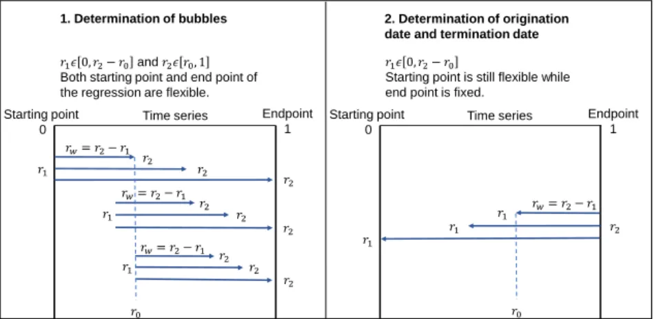
(HA:δ < 0 (stationarity)), the alternative hypothesis is of a mildly explosive process (HA:δ >0). The test is called Generalized Sup ADF (GSADF) test. As illustrated in Figure 1, the test is divided into two parts. The first part (on the left) follows the idea of repeatedly running the right-tailed ADF test on a forward expanding sample sequencerw(each sample sequence has a starting pointr1and end pointr2, the smallest sample window isr0). The test allows
varying both the starting point and the end point within a feasible range. The null hypothesis of random walk can be rejected if the largest right-tailed ADF statistic exceeds the critical value. In that case, there would be evidence of the presence of a house price bubble. The second part (on the right) is conducive to deriving both the origination and termination date of the bubble. Unlike the first part, this test is running backward and the end pointr2is fixed. The origination
date is defined as the first point in time, when the backward sup ADF statistic exceeds the critical value. Accordingly, the termination date equals to the first point in time after the origination date, when the backward sup ADF statistic falls below the critical value (Phillips et al, 2012). A minimum period between both dates should be defined to avoid that strong but only short-term fluctuations are mistakenly highlighted as bubbles (Phillips et al, 2015). For the present paper, the period should be at least 2 years.
Starting point 0 Endpoint 1 𝑟1 𝑟2 𝑟1 𝑟2 𝑟2 𝑟1𝜖 0, 𝑟2− 𝑟0 and 𝑟2𝜖 𝑟0, 1 Both starting point and end point of the regression are flexible.
Time series Time series
𝑟2 𝑟2 𝑟2 𝑟2 𝑟2 𝑟1 𝑟2 𝑟𝑤= 𝑟2− 𝑟1 𝑟𝑤= 𝑟2− 𝑟1 𝑟𝑤= 𝑟2− 𝑟1 𝑟0 𝑟1 𝑟1 𝑟1 𝑟2 𝑟1𝜖 0, 𝑟2− 𝑟0
Starting point is still flexible while end point is fixed.
𝑟𝑤= 𝑟2− 𝑟1
𝑟0
1. Determination of bubbles 2. Determination of origination date and termination date
Starting point 0
Endpoint 1
5 Structure of the Sample
Compared to other industrial countries, the availability of German house price data is restricted (Kholodilin and Michelsen, 2015). As already mentioned in the introduction, the present paper is based on regional and aggregated data provided by bulwiengesa AG and vdp.
The price data ofbulwiengesa AGreflects the price development in the whole German housing market adequately because of their high market coverage. The analysed data set covers the yearly average purchase prices and rents of newly built and second-hand apartments for 127 German cities from 1990 to 2015. Considering the number of inhabitants in the respective cities, which was also provided by bulwiengesa AG, the aggregated price development for newly built and second-hand apartments for the whole of Germany is calculated. Not all data from bulwiengesa AG are publicly available.
In contrast to bulwiengesa AG, vdp provides the price data in form of indices. In the present paper, the nominal house price indices (price index for condominiums, price index for residential rents) on aggregated level (2003/Q1– 2016/Q3) as well as for 7 cities (1991–2015) are used. Only the house price indices on an aggregated level are publicly available.
Real house prices, rents, and indices were calculated by adjusting the nominal values by the consumer price index (data from Statistisches Bundesamt). The need for seasonal adjustment was tested in R by X-13-ARIMA-SEATS from packageseasonal. According to the Root Mean Squared Error Test and the Wilcoxon Signed Rank Test, there was no significant difference between the time series before and after the seasonal adjustment. Consequently, a seasonal adjustement of the quarterly data was not necessary.
6 Examples of GSADF Test Calculation for two Cities in
Germany
The GSADF tests were carried out in EViews 9 using the add-in Rtadf
(Caspi, 2016; EViews add-ins are a possibility to provide user-defined programs to other users and can be accessed viahttp://www.eviews.com/Addins/add ins.shtml). The type of the GSADF test has to be selected as the add-in can
be used for different kinds of right-tailed ADF tests. We used theGSADF (PSY, 2015)test according to Phillips et al (2015). Within the test specifications the initial window sizer0 which is the starting point for the repeatedly running
right-tailed ADF test has to be defined. As proposed by Phillips et al (2015), the window sizer0=9 was derived from the sample sizeT =25 as follows:
r0=0.01+1.8·
√
T. (3)
Additionally, the order of the lags has to be determined. This either can be set to a fixed value or to a variable one depending on some criteria like the BIC. As proposed by Phillips et al (2015), the order of the lags was set to zero.
The critical values were calculated by Monte Carlo simulation which is one of the methods the add-in provides. To use this method, the number of replications and the significance level for the series of critical values have to be selected. We set these parameters to 2000 (following Phillips et al, 2015) and 10 %. Additonally, the parameterscandηof the data generating process (a deterministic trend) for the null hypothesis have to be specified as well:
yt =c· t Tη + t Õ j=1 j+y0. (4)
Above Equation (4) is a transformation of the general Equation given in Phillips et al (2015) and reveals the deterministic driftc·Ttη.cis the constant drift factor
andηis a coefficient which controls the magnitude of the drift. Phillips et al (2014) recommend to include a constant in the null hypothesis of the GSADF test to consider the slight drift in the price processes. Following Phillips et al (2015), we setc =η=1.
Moreover, the user can decide whether to use the fixed sample sizeT or the changing regression window sizerw in the null model. According to Caspi (2016), the latter is more accurate but, especially with larger sample sizes, quite time consuming. Nevertheless, we selectedrw.
In Table 2 the adjusted (see Equation (2)) price-to-rent ratios in the mar-ket of second-hand appartments for two German cities are provided, one of category A, the other of category D. Bulwiengesa AG classifies all Ger-man cities in a range from A to D based on influence and reach on interna-tional, nainterna-tional, regional, or local markets. For further information refer to https://www.riwis.de/online_test/en/info.php3?cityid=&info_ topic=allg.
Table 2:Prices-to-rent ratios (adjusted) of two German cities.
Year A-City D-City Year A-City D-City Year A-City D-City
1991 271.1 313.4 2001 282.0 272.6 2011 270.0 235.1 1992 282.8 274.7 2002 272.4 272.4 2012 290.0 230.7 1993 284.0 257.2 2003 270.6 260.2 2013 299.6 223.0 1994 289.4 291.7 2004 263.6 245.9 2014 315.5 226.1 1995 284.9 342.1 2005 251.6 244.3 2015 330.1 231.0 1996 303.4 329.5 2006 252.6 245.3 1997 294.3 333.5 2007 247.5 233.6 1998 291.3 313.9 2008 247.6 234.8 1999 291.0 313.6 2009 258.0 238.2 2000 290.5 305.4 2010 265.5 249.3
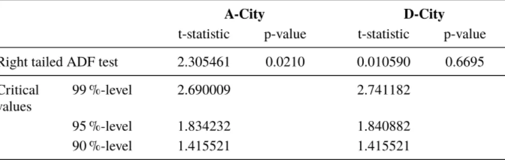
The right tailed ADF test (part one of the test procedure) for the A-city is significant to the 5 %-level, whereas the test for the D-city does not show any significance (details see Table 3). Consequently, the null hypothesis of random walk can be rejected for the A-City and there is evidence of the existence of a house price bubble in this city.
Table 3:Results of the GSADF tests for two German cities – part 1: right tailed ADF test.
A-City D-City
t-statistic p-value t-statistic p-value
Right tailed ADF test 2.305461 0.0210 0.010590 0.6695
Critical values
99 %-level 2.690009 2.741182
95 %-level 1.834232 1.840882
90 %-level 1.415521 1.415521
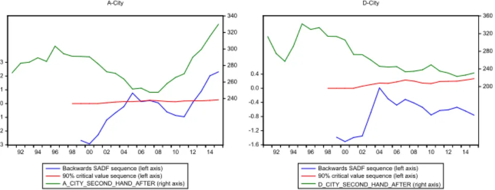
In order to identify both the origination and termination date of the bub-ble, the backward sup ADF test (part two of the test procedure) has to be applied. The results are shown in Figure 2. The green line shows the price-to-rent ratio (right axis). The blue line represents the backward sup ADF test statistics and the red line represents the critical values at 10 % significance level (both on left axis).
The origination date is defined as the first point in time when the backward sup ADF statistic exceeds the critical value. Accordingly, the termination date equals to the first point in time after the origination date when the backward sup ADF statistic falls below the critical value. In case of the A-city, there is evidence of an ongoing house price bubble emerging in 2013. In addition to that, the backward sup ADF statistic exceeds the critical value in 2005 although the price-to-rent ratio decreases from 2004 to 2005. Phillips et al (2015) emphasize that the method may falsely identify strong price decreases as bubbles as well. Thus, in order to identify real price bubbles, the development of the underlying prices has to be considered, and 2005 is not classified as a price bubble. As expected, for the D-City the backward sup ADF statistics (blue line) are lower than the critical values (red line) at every point in time.
UNTITLED01 Right Tailed ADF Tests
Sample : 1991 2015 Included observations: 25
Null hypothesis: A_CITY_SECOND_HAND_AFTER has a unit root Lag Length: Fixed, lag=0
Window size: 9 Date: 02/11/19 Time: 19:11
t-Statistic Prob.* GSADF 2.305461 0.0210 Test critical values**: 99% level 2.690009
95% level 1.834232 90% level 1.415521 *Right-tailed test
**Critical values are based on a Monte Carlo simulation (run with EVIews) UNTITLED02 -3 -2 -1 0 1 2 3 240 260 280 300 320 340 92 94 96 98 00 02 04 06 08 10 12 14 Backwards SADF sequence (left axis) 90% critical value sequence (left axis) A_CITY_SECOND_HAND_AFTER (right axis)
A-City
UNTITLED01 Right Tailed ADF Tests
Sample : 1991 2015 Included observations: 25
Null hypothesis: CITY_B_SECOND_HAND_AFTER has a unit root Lag Length: Fixed, lag=0
Window size: 9 Date: 02/04/19 Time: 16:15
t-Statistic Prob.* GSADF 0.010590 0.6695 Test critical values**: 99% level 2.741182
95% level 1.840882 90% level 1.415521 *Right-tailed test
**Critical values are based on a Monte Carlo simulation (run with EVIews) UNTITLED02 -1.6 -1.2 -0.8 -0.4 0.0 0.4 200 240 280 320 360 92 94 96 98 00 02 04 06 08 10 12 14 D-City
Backwards SADF sequence (left axis) 90% critical value sequence (left axis) D_CITY_SECOND_HAND_AFTER (right axis)
Figure 2:Results of GSADF tests for two German cities – part 2: backward sup ADF test. Left: A-City, showing a bubble, right: D-City: no evidence for a bubble.
7 Results and Discussion
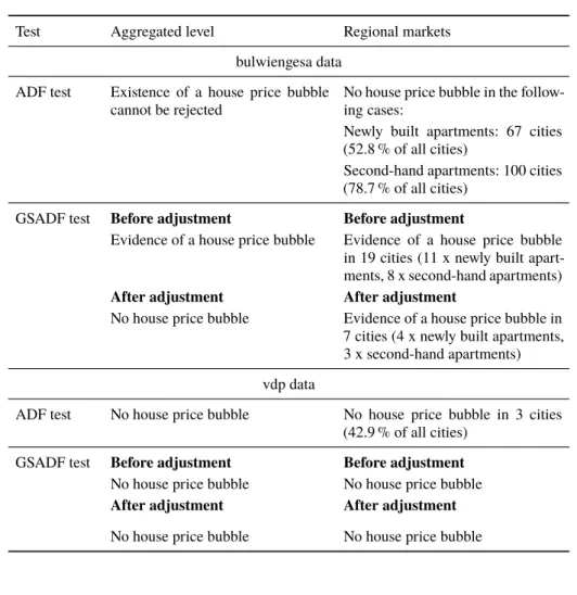
The results of the statistical tests depending on the respective data basis are explained subsequently and summarized in Table 4. It needs to be emphasized that the GSADF test aims at detecting current bubbles. Current bubbles have emerged at a given point in the time series and did not burst until the end of the time series.
Table 4:Results of the ADF and GSADF tests.
Test Aggregated level Regional markets
bulwiengesa data ADF test Existence of a house price bubble
cannot be rejected
No house price bubble in the follow-ing cases:
Newly built apartments: 67 cities (52.8 % of all cities)
Second-hand apartments: 100 cities (78.7 % of all cities)
GSADF test Before adjustment Before adjustment
Evidence of a house price bubble Evidence of a house price bubble in 19 cities (11 x newly built apart-ments, 8 x second-hand apartments)
After adjustment After adjustment
No house price bubble Evidence of a house price bubble in 7 cities (4 x newly built apartments, 3 x second-hand apartments) vdp data
ADF test No house price bubble No house price bubble in 3 cities
(42.9 % of all cities)
GSADF test Before adjustment Before adjustment
No house price bubble No house price bubble
After adjustment After adjustment
No house price bubble No house price bubble
7.1 ADF test
Theaggregateddata of bulwiengesa AG are not stationary. Hence, the existence of a price bubble cannot be rejected. However, the aggregated data of vdp are stationary. Thus, the results are ambiguous. At least, there is doubt that there is a price bubble in the entire German housing market.
Concerning theregionalmarkets, the existence of a price bubble in the time series from bulwiengesa AG can be rejected for 67 cities in the segment of newly built apartments and for 100 cities in the segment of second-hand apartments. The regional data of vdp only reflects the prices in 7 cities. The existence of a price bubble can be rejected in 3 cases.
7.2 GSADF test
According to the price-to-rent ratios based on the aggregated data of bul-wiengesa AG, there is explosive behaviour in the entire German housing market driven by the interest rate development. There is no evidence of a house price bubble in the adjusted price-to-rent ratios. Moreover, there is no explosive behaviour in the price-to-rent ratios based on aggregated data from vdp both before and after adjustment. Consequently, evidence of the existence of a Germany-wide house price bubble cannot be confirmed.
The investigation of regionalprice-to-rent ratios based on data from bul-wiengesa AG reveals that there is evidence of a house price bubble in 7 cities (4 x in the segment of newly built apartments, 3 x in the segment of second-hand apartments). In 12 additional cases, explosive price increases are driven by the interest rates. Again, the data from vdp does not indicate a price bubble.
7.3 Discussion
Besides the fact that the ADF test can only reject the existence of price bubbles, there are further points of criticism showing that the results of the ADF test are not reliable. First, this test assumes that bubbles cannot emerge again after they have burst. Thus, it is inappropriate to deal with periodically collapsing bubbles (Evans, 1991). Second, as there is a high type II error, the power of left-tailed ADF tests is quite low (Enders, 2015, pp 235).Third, the characteristics of the underlying time series must be considered to prevent distorted results (Gujarati and Porter, 2009, pp 759).
The GSADF test seems to be appropriate to detect periodically collapsing bubbles. This is proved by the results of the GSADF test regarding the housing market in the U.S. As illustrated in Figure 3, the test can detect the house
price bubble in the 2000s (emerging 1999, collapsing 2008). But, even this test cannot confirm the existence of a price bubble absolutely. Strong price increases can sometimes be reduced to factors influencing the fundamental component (e.g. interest rates). They must be considered by adjusting the fundamental component. This adjustment is necessary to detect explosive behaviour solely caused by speculation (Gürkaynak, 2008). Finally, strong price decreases are mistakenly highlighted as price bubbles (Phillips et al, 2015). The development of the price-to-rent ratio must be considered accordingly.
-5 0 5 10 15 20 80 90 100 110 120 130 1970 1975 1980 1985 1990 1995 2000 2005 2010 2015 Backwards SADF sequence (left axis)
90% critical value sequence (left axis) USA_Price_to_Rent (right axis)
GSADF test
Figure 3:House price bubble in the U.S.
Against this background and against the description of the sample structure, the results of the GSADF test based on the data from bulwiengesa AG seem to reflect the situation on the German housing market on aggregated as well as regional level adequately.
8 Conclusion
The latest global financial crisis shows that price bubbles must be detected as early as possible. The situation on the German housing market differs from housing markets in other industrial countries. Especially since 2009, real house prices and rents have been increasing significantly after a long declining or stagnating period. The GSADF test used to test for explosive behaviour indicates the existence of a house price bubble in seven German cities at the end of 2015. The ADF test, however, turns out to be neither suitable for detecting price bubbles nor reliable in rejecting them. House prices and rents continued to increase in 2016. A clear prediction of the future development is not possible, especially due to the uncertain development of interest rates. Therefore, the German housing market must continue to be closely monitored.
Acknowledgements We should like to thank the reviewers for their valuable remarks.
Appendix
60 80 100 120 140Real house price indices
2000/Q1 to 2016/Q2, 2010 = 100 2000/Q1 2002/Q1 2004/Q1 2006/Q1 2008/Q1 2010/Q1 2012/Q1 2014/Q1 2016/Q1 Germany Ireland Spain United Kingdom United States
H0: 𝛿 = 0 H0: 𝛿 = 𝛽2= 0 1. Estimation: ∆𝑃𝑡= 𝛽1+ 𝛽2𝑡 + 𝛿𝑃𝑡−1+ σ𝑖=1𝑘 𝜌𝑖∆𝑃𝑡−𝑖+ 𝜀𝑡 2. Estimation: ∆𝑃𝑡= 𝛽1+ 𝛿𝑃𝑡−1+ σ𝑖=1𝑘 𝜌𝑖∆𝑃𝑡−𝑖+ 𝜀𝑡 3. Estimation: ∆𝑃𝑡= 𝛿𝑃𝑡−1+ σ𝑖=1𝑘 𝜌𝑖∆𝑃𝑡−𝑖+ 𝜀𝑡 Yes Stationarity No H0: 𝛿 = 0 (assuming normal distribution) No stationarity Yes H0: 𝛿 = 0 H0: 𝛿 = 𝛽1= 0 Yes Stationarity H0: 𝛿 = 0 (assuming normal distribution) No stationarity Yes No No No No No Yes Yes H0: 𝛿 = 0 Stationarity No stationarity Yes No
Figure 5:ADF test procedure.
References
BIS (2016) International banking and financial market developments. BIS Quarterly Review September.
Brunnermeier MK, Oehmke M (2013) Bubbles, Financial Crises, And Systemic Risk. Handbook of the Economics of Finance 2(PB):1221–1288. DOI: 10.1016/B978-0-44-459406-8.00018-4.
Caspi I (2016) Rtadf: Testing for Bubbles with EViews. URL:http://econ.biu. ac.il/files/economics/shared/riedp_4-16.pdf.
Deutsche Bundesbank (2016) Monetary policy and banking business. Monthly Report, pp. 25–38.
Deutsche Bundesbank (2017) Economic conditions in Germany. Monthly Report, pp. 44–55.
Diba BT, Grossman HI (1988a) Explosive Rational Bubbles in Stock Prices? American
Economic Review 78(3):520–530. URL:https://www.jstor.org/stable/
1809149.
Diba BT, Grossman HI (1988b) The Theory of Rational Bubbles in Stock Prices. The Economic Journal 98(392):746–754. DOI: 10.2307/2233912.
Dolado JJ, Jenkinson T, Sosvilla-Rivero S (1990) Cointegration and Unit Roots. Journal of Economic Surveys 4(3):249–273. DOI: 10.1111/j.1467-6419.1990.tb00088.x
Dombret A (2016) Blase oder nicht – wo steht der deutsche Wohnimmobilienmarkt? ifo Schnelldienst 69. Jg.(August):20–25.
Dreger C, Kholodilin KA (2013) Zwischen Immobilienboom und Preisblasen: Was kann Deutschland von anderen Ländern lernen? DIW Wochenbericht 17:3–10. Empirica AG (2017) Blasenindex IV/2016. empirica-Preisdatenbank Februar. Enders W (2015) Applied Econometric Time Series, 4th edn. Wiley, Hoboken, NJ,
USA.
Evans GW (1991) Pitfalls in Testing for Explosive Bubbles in Asset Prices. American Economic Review 81(4):922–930.
Gilles C, LeRoy SF (1992) Bubbles and Charges. International Economic Re-view 33(2):323–339. DOI: 10.2307/2526897.
Gujarati DN, Porter DC (2009) Basic Econometrics, 5th edn. McGraw-Hill, New York, USA.
Gürkaynak RS (2008) Econometric tests of asset price bubbles: Taking stock. Journal of Economic Surveys 22(1):166–186. DOI: 10.1111/j.1467-6419.2007.00530.x Hamner B, Frasco M (2017) Metrics: Evaluation Metrics for Machine Learning.
URL:https://CRAN.R-project.org/package=Metrics. R package ver-sion 0.1.3.
Helbling TF (2005) Housing price bubbles - a tale based on housing price booms and busts. BIS Papers 21:30–41, Bank for International Settlements. URL:https:// EconPapers.repec.org/RePEc:bis:bisbpc:21-04.
Homm U, Breitung J (2012) Testing for speculative bubbles in stock markets: A com-parison of alternative methods. Journal of Financial Econometrics 10(1):198–231. DOI: 10.1093/jjfinec/nbr009.
Kholodilin K, Michelsen C (2015) Weiter steigende Immobilienpreise, aber keine flächendeckenden Spekulationsblasen. DIW-Wochenbericht 82(49):1164–1173. Kholodilin K, Michelsen C, Ulbricht D (2015) Speculative Price Bubbles in Urban
Housing Markets in Germany. Discussion Papers DIW Berlin 1417:1–31.
Kivedal BK (2013) Testing for rational bubbles in the US housing market. Journal of Macroeconomics 38(PB):369–381. DOI: 10.1016/j.jmacro.2013.08.021.
McLeod AI, Yu H, Mahdi E (2012) Time Series Analysis with R. Handbook of Statistics 30:661–712.
Michelsen C, Weiß D (2009) What Happened to the East German Housing Market? – A Historical Perspective on the Role of Public Funding –. IWH-Discussion Papers 20. Pfaff B (2008) Analysis of Integrated and Cointegrated Time Series with R, 2nd edn. Springer, New York. URL:http://www.pfaffikus.de. ISBN 0-387-27960-1. Phillips PCB, Wu Y, Yu J (2011) Explosive Behavior in the 1990s NASDAQ: When Did
Exuberance Escalate Asset Values? International Economic Review 52(1):201–226. DOI: 10.1111/obes.12026.
Phillips PCB, Shi S, Yu J (2012) Testing for Multiple Bubbles. Cowles Foundation Discussion Paper 1843:1–66.
Phillips PCB, Shi S, Yu J (2014) Specification Sensitivity in Right-Tailed Unit Root Testing for Explosive Behavior. Oxford Bulletin of Economics and Statis-tics 76(3):315–333.
Phillips PCB, Shi S, Yu J (2015) Testing for Multiple Bubbles: Historical Episodes of Exuberance and Collapse in the S&P 500. International Economic Re-view 56(4):1043–1079. DOI: 10.1111/iere.12132.
R Core Team (2017) R: A Language and Environment for Statistical Computing. Vienna, Austria. R Foundation for Statistical Computing, Vienna, Austria. URL:https:// www.R-project.org/.
Reinhart CM, Rogoff KS (2008) Is the 2007 US Sub-Prime Financial Crisis So Different? An International Historical Comparison. American Economic Review 98(2):339–344. DOI: 10.1257/aer.98.2.339.
Sax C (2017) seasonal: R Interface to X-13-ARIMA-SEATS. URL:https://CRAN. R-project.org/package=seasonal. R package version 1.6.1.
Scherbina A (2013) Asset Price Bubbles: A Selective Survey. IMF Working Pa-pers 13(45):1–40. DOI: 10.5089/9781475515299.001.
Scherbina A, Schlusche B (2012) Asset Bubbles: An Application to Residential Real Estate. European Financial Management 18(3):464–491. DOI: 10.1111/j.1468-036X. 2012.00647.x
Stiglitz JE (1990) Symposium on Bubbles. Journal of Economic Perspectives 4(2):13–18. DOI: 10.1257/jep.4.2.13.
Tissot B (2014) Monitoring house prices from a financial stability perspective - the BIS experience. In: IFC-sponsored sessions at the ISI Regional Statistics Conference 2014, Bank for International Settlements. URL:https://www.bis.org/ifc/ events/ISI_reg_stats_conf2014/session4_BISpaper.pdf.
Trapletti A, Hornik K (2017) tseries: Time Series Analysis and Computational Finance. URL:https://CRAN.R-project.org/package=tseries. R package ver-sion 0.10-42.
Wu Y (1997) Rational Bubbles in the Stock Market: Accounting for the U.S. Stock-Price Volatility. Economic Inquiry 35(April):309–319. DOI: 10.1111/j.1465-7295.1997. tb01912.x