Study of Shock Wave Boundary Layer Interaction Using Pressure-Sensitive Paint
Thesis
Presented in Partial Fulfillment of the Requirements for Graduation with Distinction in the College of Engineering of The Ohio State University
By
Matthew William Frankhouser
Undergraduate Program in Aeronautical and Astronautical Engineering
The Ohio State University 2013
Thesis Committee
Professor James W. Gregory, Advisor Professor Michael Dunn
Copyright by
Matthew William Frankhouser 2013
ii Abstract
Through the advancement of aviation, engineers and designers have strove to improve the performance of aircraft and push through the various flight regimes. As aircraft encounter transonic flight, compressibility effects begin to impose limitations and impede their performance. One such limitation comes from the shock wave boundary layer interaction, also known as buffeting, that occurs on the wings of aircraft but more so on the blades of rotor-craft. Prior work in this study has investigated the effects on oscillating free stream Mach numbers on a NACA0012 airfoil due to its relevance to helicopter aerodynamics. These studies were conducted with the airfoil at a fixed angle of attack with the Mach number set to oscillate in and out of the known buffet conditions. By oscillating the flow with a rotating cam, the Mach number can be forced to mimic the periodically varying freestream velocity conditions that a rotor blade would experience in forward flight. In these experiments the presence of oscillatory shock waves at high subsonic speeds and their physical mechanisms are not fully understood. This experiment sets out to use Pressure Sensitive Paint (PSP) as a method of detecting buffet on the surface of an airfoil by obtaining global surface pressure distribution in transonic flight conditions. The tests include steady runs as a baseline as well as oscillatory free stream velocity fields on a NACA 0012. The pressure taps were used to validate the PSP results. A fast-acting single-luminophore pressure sensitive paint applied to a polymer-ceramic basecoat was chosen for the experiments. The PSP measurements were made using an intensity-based pressure-sensitive paint technique that utilized a high-speed camera and Ultra-Violet LED arrays. This technique allows for accurate unsteady pressure
iii Dedication
iv
Acknowledgements
I sincerely thank my advisor, Dr. James Gregory, for the opportunities he has granted me in conducting this research as an undergraduate.
My family has always strongly support me through my endeavors. My parents and brothers have always supported me through my endeavors. I thank them for the unwavering support, guidance, and motivation that they have provided.
For their insight and assistance, I thank the various members of the lab group. I want to give a special thanks to Kyle Gompertz for the generous contribution of his time, and to Kyle Hird for his technical assistance in post-processing the data.
Finally, I am grateful to the College of Engineering for the financial support to conduct this work.
v Vita
December 13, 1990……… Born, Salem, Ohio, USA
May 21 , 2009………West Branch High School; Beloit, Ohio May 5, 2013……… B.S., Aeronautical and Astronautical
Engineering, The Ohio State University
Fields of Study Major Field: Aeronautical and Astronautical Engineering
vi Table of Contents Abstract………...… ii Desication………... ii Acknowledgements………....… iv Vita………... v Field of Study………..….... v Table of Contents………...… vi
List of Tables………... viii
List of Figures………..… viii
List of Equations………. x
Chapter 1: Introduction………..…. 1
Pressure Sensitive Paint………..… 3
Chapter 2: Experimental Facility……….... 5
Mach Oscillation………..…….. 8
Data Aqusition……….…. 10
Experimental Airfoil………. 11
Pressure Sensitive Paint Measurement Technique………..………. 13
Chapter 3: Data Acquisition……….….…... 14
Image Registration……….….. 15
Pressure and Temperature Correction………..………...… 16
Chapter 4: Results………....…… 21
vii
10-degree Angle of Attack with Mach Oscillation……….26
9-degree Angle of Attack with Mach Oscillation………..……… 35
Errors………. 44
Chapter 5: Conclusion………..…. 45
Chapter 6: Future Work………. 46
References……….… 47
Appendix A: Normal Shocks……… 49
viii List of Tables
Pressure Tap Locations………. 13
Peaks and local minimums for four cycle………. 38
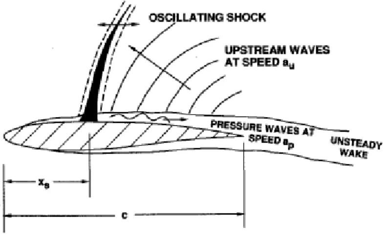
List of Figures Figure 1: Schematic diagram of shock oscillations……… 2
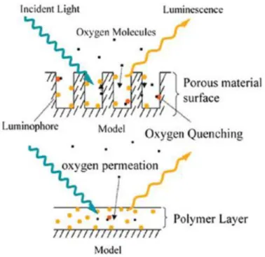
Figure 2: Schematic of porous binder (Top) compared to conventional PSP (bottom)…. 5 Figure 3: Schematic diagram of the Aeronautical and Astronautical Research Laboratory 6”x22” Transonic Wind Tunnel……….. 6
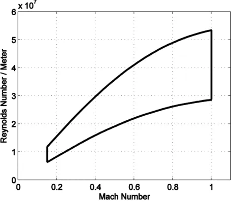
Figure 4: Range of test section operation conditions for the 6”x22” Transonic Wind Tunnel……….. 7
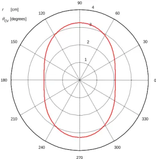
Figure 5: Geometry of Rotation Turning Vane……….… 8
Figure 6: Freestream Waveform………...……….… 9
Figure 7: Mach Oscillation Drive Train Assembly………. 10
Figure 8: NACA 0012 airfoil with PSP applied……….. 12
Figure 9: Data acquisition for real-time method………. 14
Figure 10: Wind-off image (left) wind-on image (right)……… 15
Figure 11: Wind-on registered image……….… 16
Figure 12: Error in percent of between temperature correction methods…………. 18
Figure 13: PSP a priori calibration surface fit………... 19
Figure 14: Chordwise PSP and pressure tap data……….. 20
Figure 15: Evaluation of three test cases………..……. 25
ix
Figure 17: 10-degree Mach oscillation normalized standard deviation………... 27
Figure 18: Cp surface distribution at discrete spatial locations………... 28
Figure 19: Cp at different span locations………. 29
Figure 20: Mach number at different span locations………... 30
Figure 21: Normal shock capture……… 32
Figure 22: Standard deviation vs Mach number over ten cycles………. 33
Figure 23: Standard deviation of Cp vs Reynolds number over ten cycles………. 33
Figure 24: SD of Cp vs Mach showing unset of buffet detection………... 34
Figure 25: Standard deviation normalized by the mean, Mach number, and Reynolds number as a function of time……… 36
Figure 26: Zoom in on Figure 20, showing portion of oscillation between 1.5 and 1.9 seconds……… 37
Figure 27: Locations of Interest in 9-degree oscillation case………. 37
Figure 28: Number locations of images for 9-degree angle of attack with Mach oscillation……… 40
Figure 29: Images corresponding to locations on Figure 28……….. 41
Figure 30: 9-degree angle of attack SD vs Mach with Mach oscillation…………...… 42
x
List of Equations
Equation 1: Stern-Volmer Equation……… 3
Equation 2: Time response of PSP……….. 4
Equation 3: Mach number Area ratio relationship……….. 7
Equation 4: Isentropic pressure equation………..… 22
Equation 5: Reynolds number………... 22
Equation 6: Ideal Gas Law……… 22
Equation 7: Isentropic Relation……… 23
Equation 8: Isentropic temperature equation……… 23
Equation 9: Sutherlands Law……… 23
Equation 10: Speed of sound……… 23
Equation 11: Mean value ………. 23
Equation 12: Standard Deviation……….. 24
xi Nomenclature
= choke area R = specific gas constant
= throat area Re = Reynolds number
A= speed of sound SD = standard deviation
b = airfoil span T = temperature
c = airfoil chord = total temperature
= coefficient of pressure = static temperature = critical coefficient of pressure γ = ratio of specific heats = mean coefficient of pressure ρ = density
M = Mach number = total density
P = pressure μ = viscosity
= total pressure = total viscosity = static pressure
1
Chapter 1: Introduction
The mechanisms of dynamic stall have been widely investigated. Two methods have been produced to investigate different flow qualities, varying the freestream velocity or airfoil pitch during the experiment. These particular methods had been used to evaluate helicopter blades. By varying the angle of attack, the cyclic pitching of the blades is simulated, while varying the freestream Mach number replicates the flow seen by rotorcraft during forward flight.
For this investigation, the airfoil was held at a constant angle of attack while sinusoidally varying the freestream velocity. This particular method has previously been used in investigations to evaluate helicopter blades, which encounter similar sinusoidal variations in freestream Mach number. The varying Mach number leads to the
development of an unsteady shock wave that varies in position and strength on the airfoil. These various studies have demonstrated that shock wave interaction with a separated boundary layer is directly associated with many unsteady phenomena1. These shock oscillations result in pressure fluctuations which result in unwanted stress applied to the airfoil, noise, and shock-induced flow separation.
2
Figure 1: Schematic diagram of shock oscillations8
Numerous investigations have been conducted by Babinsky, Fernie, and Bruce3-7 which have examined the dynamic effects of unsteady freestream oscillations on a NACA-0012 airfoil at low angles of attack. Their results concluded that differences in shock location and strength were influenced by and depend on the free-stream Mach number and whether it is increasing or decreasing. The decelerating free-stream Mach number induced a stronger shock which moved forward, while the accelerating free-stream at the same Mach number induced a weaker shock. Their measurements included kulite data acquired from the airfoil surface and Schlieren images to capture the dynamic flow qualities. Their research demonstrated the forced shock oscillations can be generated and analyzed.
Buffeting has been defined as a self induced unsteady interaction between the shock wave and boundary layer, shock oscillations on the surface of an airfoil which occurs in the transonic regime2. This phenomenon is highly three-dimensional and
drastically affects the performance of aircraft. As the flow encounters the shock wave, the flow’s velocity is decreased, while the pressure is increased, which can lead to boundary
3
layer separation. This shock induced separation changes the effective geometry of the airfoil which contributes to the random motion of the shock2.
Pressure Sensitive Paint Introduction
PSP is an optical measurement technique used for measuring the global surface pressure distribution on an experimental model. This experimental technique is based on the light intensity emitted by oxygen quenching of luminescence molecules. Compared to conventional pressure measurement techniques, such as pressure taps or pressure
transducers, PSP offers the capability of high frequency pressure measurements with fine spatial resolution that is less intrusive to the flow. A light source is needed to excite the oxygen-sensing molecule, known as a luminophore, which is painted in a permeable paint binder12. The luminescent molecules respond to the excitation light source by emitting a longer wavelength light. The intensity of the emitted light is influenced by the oxygen quenching process, which is inversely proportional to the amount of oxygen in the surround air as well as the temperature of the model12. The measured emitted light intensity can then be converted to a pressure measurement using the Stern-Volmer Equation, where A and B are the Stern-Volmer coefficients found during the a priori
calibration.
Equation 1: Stern-Volmer Equation
P
P
(T)
B
+
(T)
A
=
ref refI
I
4
Due to the unsteady compressible flow field, a fast responding single luminophore, platinum porphyrin PSP was used. To capture the rapid pressure
fluctuations on the model, a porous binder was used to increase the oxygen quenching. The response time is determined by the amount and rate of oxygen diffusion into the paint layer. This paint response time is characterized by, Equation 2 where is the response time, h is the binder thickness, and D is the diffusion coefficient of the binder layer.
Equation 2: Time response of PSP
D
h
2
By utilizing the porous binder, the luminophore molecules are more accessible to the oxygen molecules, which reduces the response time compared to non-porous paint binders.
For a typical tunnel entry, the run durations would last four to seven seconds with data being acquired for three to five seconds. For these short durations, the real-time data acquisition method was used to obtain PSP pressure measurements. A real-time method utilizes a high-speed camera with a frame rate that is sufficient to capture the unsteady pressure fluctuations12. This method does not require sophisticated triggering or phase locking systems to capture images. However, this method does require a high-power continuous excitation source to allow for the short exposures necessary to obtain the transient flow phenomenon.
5
Figure 2: Schematic of porous binder (top) compared to conventional PSP (bottom)9
Chapter 2: Experimental Facility
The experiments were conducted in the Ohio State University’s 6” x 22” transonic wind tunnel at the Aeronautical and Astronautical Research Laboratory. The tunnel (Figure 3) is a blow down tunnel that is supplied with air by two 21 m3 tanks that can be pressurized up to 15.5 MPa. Two values are situated upstream of the settling chamber; the first is a control valve that sets the pressure and Reynolds number18. The second valve is a fast-acting valve that is used to start and stop the flow.
6
Figure 3: Schematic diagram of the Aeronautical and Astronautical Research Laboratory 6”x22” Transonic Wind Tunnel18
The wind tunnel was specifically designed for low turbulence; this is achieved as the flow passes through the settling chamber of the tunnel. To lower the turbulence to 0.5%, as the flow enters the settling chamber, it passes through a perforated plate, honeycomb, and five screens of mesh10. The subsonic nozzle contracts the flow into the test section, where perforated plenums are placed at the top and the bottom of the test section to reduce Mach wave reflections in transonic flow conditions18.
The Mach number is set by varying the throat area downstream of the test section. This allows for the Mach number and Reynolds number to be independently selected over a wide range.
7
Figure 4: Range of test section operation conditions for the 6”x22” Transonic Wind Tunnel
Run durations for this experiment lasted 5 seconds with 20 to 30 minutes between runs for the tank pressure return to the desired level.
The Mach number is determined by the Mach-area ratio equation. A series of varying-diameter bars are inserted into the tunnel, downstream of the test section, to set the Mach number during the steady flow field conditions.
Equation 3: Mach number Area ratio relationship
21 1 2 * 2 1 1 1 2 M M A A t
8
Mach Oscillation
For the Mach oscillation experiments, the oscillations were produced by rotating four elliptical cams, which are located downstream of the test section, at 5 Hz. By oscillating the vanes and changing the effective throat area, pressure perturbations move upstream from the vanes to the test section18. These pressure waves correspond to the Mach number variation. The elliptical vanes were designed to produce a sinusoidal oscillation in Mach number to mimic free stream conditions of a rotorcraft in forward flight. The turning vanes are constructed in two pieces that fit over a square shaft and then are bolted together.
Figure 5: Geometry of Rotating Turning Vane
1 2 3 4 30 210 60 240 90 270 120 300 150 330 180 0 r [cm] CV [degrees]
9
Figure 6: Freestream Waveform
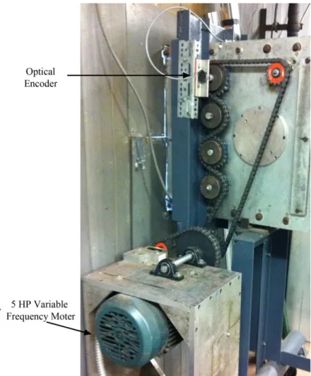
The choke vanes are driven by a 5-HP alternating-current electric motor through a drive-chain mechanism. Each vane is linked to the motor by the drive chain. The vanes are counter rotating to obtain the proper periodic oscillations within the test section. An optical encoder is mounted to the top vane to record the frequency of rotation. The encoder had three channels, two 2500 per revolution and a once per revolution. The signals were processed in LabVIEW to calculate the degree of rotation of the vanes throughout the run. At 10 Hz, the freestream flow field does not follow the analytical waveform. The discrepancies between the experimental and analytical waveform can be accounted for by the high frequency of the rotating cams, and from slight misalignments of the four cams as they are installed in the wind tunnel.
10
Figure 7: Mach Oscillation Drive Train Assembly
Data Acquisition
During the run, a system of three computers was used to record the necessary data. One computer recorded the voltage signals from the various measurement devices, one operated the high-speed camera, and one operated the pressure scanners used to record the pressure tap data.
The first computer operated a LabVIEW code which controlled a BNC data acquisition board (DAQ board) and a quadrature board. The quadrature board obtained
11
the three signals from the optical encoder that was used to record the position of the choke vanes. The BNC DAQ board acquired voltage signals from two pressure transducers, one that recorded the stagnation pressure of the tunnel and another which recorded the static pressure in the test section. In addition the transducers, two voltage signals from thermistors on the airfoil were recorded for temperature data. Two trigger signals were generated from the BNC DAQ board; one signal was supplied to the high-speed camera to start recording images and the other to the pressure scanners to record pressure tap data. The shutter signal from the camera was also recorded and used to correlate the images to the phase of the turning vane and the free stream Mach number.
The second computer operated the high-speed camera software. The signal from the DAQ board started the recording process, in which the camera recorded for 5 seconds at 1000Hz.
The third computer operated the software for the pressure scanners and saved the data. The computer obtained the trigger signal from the BNC board; the trigger signal was used to start a square wave that was in phase with the shutter of the camera. The rising edge of the square wave triggered the software to record pressure tap data from the airfoil.
Airfoil
From prior experiments, typically a NACA 0012 airfoil is used because of its relevance to helicopter rotor blades. For this reason a NACA 0012 was chosen to directly verify results against published data. The airfoil is partially hollow to allow access for the
12
pressure tap tubing and thermistor wires. This particular airfoil is capable of pitch oscillation and is fitted with a cylindrical mount that is inserted into a bearing. Two thermistors are mounted, one each near the leading and trailing edges, and are used to correct the model temperature distribution due to the varying thickness of the airfoil. There are 14 pressure taps on the airfoil: 2 taps on the lower surface and 12 taps on the upper surface. These taps are used to apply the in situ calibration to the PSP. The PSP used for this experiment was a single-luminophore platinum porphyrin (PtTFPP) paint.
13
Table 1: Pressure Tap Locations
Upper Surface x/c 0.050 0.100 0.150 0.250 0.300 0.350 0.400 0.500 0.700 0.900 z/b 0.583 0.583 0.583 0.500 0.583 0.667 0.750 0.583 0.583 0.583 Lower Surface x/c 0.100 0.500 z/b 0.583 0.583
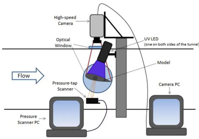
Pressure Sensitive Paint Measurement Technique
The 6” x 22” wind tunnel has three optical windows in the test section that were used to acquire PSP data. One window is located on each side of the airfoil, and the third is located directly above the test section. One LED array was mounted to each side of the tunnel and utilized the side window to illuminate the airfoil. The 3-watt LED arrays emitted 405nm-wavelength light that is optimal for the PtTFPP luminophore excitation. Each LED was situated so that the light field from each array was as close to
perpendicular to the airfoil surface as possible. The high-speed camera was mounted above the tunnel and used the window above the test section to capture the surface of the airfoil. A phantom high-speed CMOS (complementary metal oxide
semiconductor)camera was used to capture the images at 1000 Hz with an exposure time of 965μs. With this frame rate and exposure time, the maximum resolution of which the camera was capable was 1280x800 pixels. The high-speed imaging allows the dynamic flowfield to be captured in a short time, which minimizes the temperature variations present on the model and reduces photodegradation. A red channel 590nm optical long
14
pass filter was placed on the camera lens to filter out the excitation light, allowing only the paint emission to be captured.
Figure 9: Data acquisition for real-time method
Chapter 3: Data Acquisition
All the saved data on the data acquisition, pressure scanner, and high-speed camera computers were transferred onto an external hard drive for postprocessing. From the data acquisition computer, the values of the encoder were used in determining the angular position of the turning vanes as well as the number of cycles per run. The shutter signal from the camera was used to synchronize the images to the correct pressure
15
transducer and thermistor signals, as well as the pressure scanner values. This data was used to calculate Mach number over the duration of the run.
Image Registration
For the PSP images to be processed in order to determine the coefficient of pressure, they first needed to be registered. Registration of the images ensures that all the images are spatially aligned to a fixed position in the image. For PSP measurements, a series of images need to be taken which include dark images of the model in the tunnel, wind-off illuminated images of the model, and wind-on illuminated images of the model. During the wind tunnel entries, flexing of the tunnel walls due to pressurization of the tunnel and oscillations of the camera from vibrations leads to misalignment of the images. In order to properly ratio the wind-off to the wind-on images, the image alignment is crucial.
Figure 10: Wind-off image (left) wind-on image (right)
The alignment process begins with the creation of a mask around the airfoil. This was achieved by averaging all the images over the length of the wind-off run. The surrounding edges of the airfoil were edited and turned a solid black with the inside
16
depicting just the airfoil to create the mask. An image registration code that utilized a two-dimensional cross correlation was then used to align the wind on and wind off images to the bounding edges of the mask and to the pressure taps on the surface of the airfoil, ensuring each image lined up spatially. These registered images were then cropped to show only the airfoil surface.
Figure 11: Wind-on registered image
Pressure and Temperature Correction
An a priori and an in situ calibration were performed on the PSP for more accurate pressure results. The a priori calibration method utilizes a pressure and
temperature calibration chamber to record the emission intensity of a PSP sample and the temperature and pressure of the chamber for each reference point in the steady
calibration. A matrix of pressure and temperature set points are input into the LabVIEW system and the pressure and temperature controllers independently control the chamber
17
conditions. Each image of the PSP sample is divided by the reference intensity to
calculate the intensity ratio for each individual set point of pressure and temperature. The
a priori calibration assumes a uniform temperature and pressure distribution, which is not indicative of the experiment. During the wind-on tunnel tests, the pressure and high-Mach number freestream flows around the aluminum airfoil, inducing a temperature gradient on the airfoil which varies in magnitude between each run.
Since this was a single-luminophore paint with only the ability to detect pressure, there existed a temperature bias. To correct for the temperature, infrared (IR) images taken of the same model at similar test conditions were obtained from previous
experiments. These images contained the temperature gradient of the NACA 0012 airfoil and were used as a base temperature map for the airfoil. The thermistor data was used to perform a bulk shift of the IR temperature map to match the model temperature to each PSP image.
Along with using the IR data to perform the temperature correction, a linear temperature gradient was also assumed between the two thermistors. Since the IR data had not come directly from the same atmospheric conditions, the linear gradient served as a check with the IR data. Using both IR and the linear temperature gradient to correct for the temperature, the pressure surface map was calculated along with the error obtained from both methods of temperature correction.
18
Figure 12: Error in percent of between temperature correction methods. The two methods agree nicely. The areas of highest error occur near the leading edge and the sides of the airfoil. These areas are known to have lighting non-uniformity. At the leading edge, the curvature of the airfoil does not allow for the light source to be
perpendicular to the surface, which results in lower illumination intensity. Near the edges of the airfoil, reflections from the sidewalls of the tunnel interfere with the intensity emission of the PSP.
An in situ calibration method was used for calibrating the PSP a priori intensity ratio to the pressure taps on the supper surface of the model. The in situ method creates a surface fit calibration for the pressure with respect to the intensity ratios of the wind-on and wind-off images. This was achievable due to the use of the high resolution pressure scanners that were synchronized to the camera shutter. With the use of the
single-luminophore PSP, the in situ calibration was required for each image due the variations in the temperature field of the model. The a priori surface sit calibration used in the in situ
19
pressure for the airfoil surface can be directly found for each image of the steady and unsteady runs by using the Stern-Volmer Equation (Equation 1).
20
Figure 14: Chordwise PSP and pressure tap data
Applying the a priori calibration fit to the PSP images does not accurately fit the PSP pressure results to the pressure tap data. The a priori is the first step taken to obtain the pressure distribution on the airfoil. Next the in situ calibration is applied individually to each image using the pressure tap data corresponding to that image. This accurately correlates the PSP image results to the exact pressure acquired from the pressure taps, yielding a highly accurate pressure distribution on the airfoil. Figure 14 indicates that at a location of 30% chord that the PSP deviates from the pressure tap data. This deviation arises from temperature gradients and illumination intensity. Towards the trailing edge, the airfoil thickness begins to decrease. This decrease in thickness, coupled with the thermal properties of aluminum, contribute to larger surface temperature variations. In
21
addition to the temperature, only two 3watt LED arrays were used to illuminate the airfoil. The flow instabilities that were investigated in this research occur at chordwise locations between 0 and 30 percent of the chord. To capture the flow phenomena, the LED’s were placed to provide maximum illumination to the leading edge, thus resulting in a poor illumination field aft of 30% chord.
Chapter 4: Results
The NACA 0012 airfoil was tested at two different tunnel conditions, steady and unsteady oscillating freestreams. In the oscillating freestream cases, the airfoil was held fixed at two different angles of attack, 9 and 10 degrees. The resultant Mach oscillation varied the freestream velocity in a periodic waveform. The oscillations occurred at 10 Hz with a minimum and maximum Mach number of 0.485 and 0.581 respectively. For the 10-degree case, the NACA 0012 should be at the onset of buffeting at Mach numbers greater than 0.57. At the 9-degree case, buffet should not occur within this Mach range. For the unsteady testing, the steady cases served as baseline and for verification of results. These involve a 10-degree case at Mach 0.54 and a 9-degree case of 0.54. For all tests, the high speed camera recorded images at 1000Hz with a resolution of 1280x800 pixels.
Numerical Calculations
Numerical data was obtained as voltage signals acquired by the DAQ boards as well as the pressure data from the airfoil pressure taps. For all the calculations, was assumed to be the atmospheric conditions at the time of each test. The Mach number for each image was calculated using and that were directly measured with the pressure
22
scanner from taps in the tunnel. The tap for is located inside the settling chamber, while the tap was located 22 inches in front of the airfoil. The phase lag of the pressure waves propagating from the turning vanes was accounted for based on the spatial locations of each tap relative to the airfoil. The isentropic equation relating and
to the Mach number was rearranged to solve for Mach number. The Mach number was calculated using Equation 4, the isentropic equation relating the pressure ratio to the Mach number. The Reynolds number is acquired by Equation 5, which was dependent on ρ and μ which oscillate with tunnel conditions. To calculate Reynolds number, was calculated using Equation 6, using the and . Next, ρ was calculated with Equation 7. To calculate the viscosity, μ was calculated using Equation 9, and the temperature for Equation 9 was calculated using Equation 8. The velocity was determined by calculating the speed of sound with Equation 10 and multiplying by the Mach number. With all the necessary values found, the Reynolds number was calculated for each image during the tests.
Equation 4: Isentropic pressure equation
( )
Equation 5: Reynolds number
Equation 6: Ideal Gas Law
23 Equation 7: Isentropic Relation
( )
Equation 8: Isentropic temperature equation
( )
Equation 9: Sutherlands Law
( ) (
) Equation 10: Speed of sound
√
Numerical calculations were also performed using the distributions obtained from the PSP images. For all the images, only the leading edge was selected due to light concentration and non-uniformity of the light from the tunnel. With the surface map, the standard deviation (SD) and for each row of pixels was calculated to obtain a single value for reach row.
Equation 11: Mean value
24 Equation 12: Standard Deviation
√ ( ) ( ) ( )
( )
The SD will be used to determine if shock/boundary layer interactions have occurred. With the inherent pressure increase across a shock wave, fluctuations in the SD should indicate that instability has formed on the airfoil. Because of the direct dependency on the Mach number oscillations the SD showed the periodic waveform. To correct for this, and level the periodic variations, the value was normalized by . The normalization of the SD also emphasizes the sharp variations that would occur if an instability was captured.
25
Figure 15: Evaluation of three test cases
Analysis of these three different test conditions over 500 ms provides evidence of what was expected in each case. For the steady test at 10 degrees angle of attack at a Mach number of 0.54, the normalized standard deviation only contains noise throughout the run. The 9-degree unsteady case, at the higher Mach numbers, shows that there is a repeatable three bump pattern that occurs. In comparison, the 10-degree unsteady case does not show signs of a pattern and contains large random spikes in the normalized standard deviation.
26
10-degree Angle of Attack with Mach Oscillation.
Figure 16: 10-degree with Mach oscillation
Figure 16demonstrates the oscillation in standard deviation normalized by the mean coefficient of pressure and the Reynolds number follows the same oscillatory pattern at the frequency at which the freestream Mach number is driven. This is what would be expected in the unsteady tests.
27
Figure 17: 10-degree Mach oscillation normalized standard deviation
By viewing only five cycles at a time in the 10 degree unsteady case, the sharp spikes can be seen in the normalized SD. These variations tend to be more rapid with larger deviation during the decelerating portion of the Mach oscillation. This coincides with finds of Babinsky et al3-7 that found stronger shocks occurred during the
28
Figure 18: Cp surface distribution at discrete spatial locations
The above figure (Figure 18) shows images during a spike in the normalized SD. The blue squares in the figures above the images correspond to the images from left to right respectively. From the figures and the images, the sharp drop in the normalized SD indicated that an instability has occurred. These strong shocks occur rapidly, in both spatial locations, the time span from the shock at its strongest to not being present takes
29
approximately 3ms; the duration of the shock forming to fading takes approximately 7ms. At these conditions, the onset of shock/boundary layer interaction should start to begin. These rapid instabilities appear to last for a short time on the surface of the airfoil.
To investigate the nature of these further, the distributions along different spanwise locations are plotted in Figure 19. The plots correspond to the images directly beneath them.
Figure 19: Cp at different span locations
The critical coefficient of pressure ( ) was calculated using Equation 13 Equation 13: Critical coefficient of pressure
([
( ) ]
)
The first image serves as a reference condition. The freesteam is the lowest attainable Mach number during the run. For this image, the plotted values were taken
30
from x/b = 0.73. This is what a typical curve should look like for an airfoil at these conditions. The second image coincides with a spike in the normalized SD. The figure plots two spanwise locations. The red trace is directly in the middle of the “wedge shaped instability” (z/b = 0.62) that has occurred near the trailing edge, and the blue trace is offset in a region that is undisturbed from the wedge. From the plotted data for z/b=0.62, there is a plateau in the that extends from x/c=0.08 to 0.2. This indicates that a
separation bubble has formed in this location and has affected the boundary layer; this separation bubble appears to be caused by a weak shock near the leading edge. The third figure has the same formatting as the second with the red trace taken in the middle of the wedge (z/b=0.79) and the blue trace taken from a region that is not affected by the
instability (z/b=0.56). Similar to the second figure, there is a plateau in . What differs between them is that instead of a level plateau, there is a decrease in around
x/c=0.05 with a slight increase before the – decreases over the rest of the length of the airfoil. Also, the spanwise location associated with the boundary layer interference (z/b=0.79), does not recover to the same as the offset data set (z/b=0.56). This could indicate that a shock has occurred near the leading edge which corresponds to the initial increase in ; the slight decrease following could be the boundary layer reattaching to the surface of the airfoil.
In both images for the spanwise location where there is no disturbance (the blue traces), around x/c = 0.12 there is a sharp drop in . This could be associated with a shock that has formed. With the NACA 0012 pitched to an angle of attack of 10 degrees at this range of Mach numbers, the on the surface of the airfoil are above the .
31
In the third plot, the flow represented by the blue trace undergoes attached flow diffusion on the aft portion of the airfoil. Since the flow is attached at this spanwise location, the boundary layer is thin. Thus the flow accelerates to high speeds around the upper surface near the leading edge. This corresponds to a strong normal shock
positioned relatively far downstream on the airfoil surface. This shock is not stable at this condition near the buffet boundary. The red trace indicates that there is a closed
separation bubble spanning from approximately x/c=0.05 to x/c=0.25. The bubble reattachment occurs gradually and does not suddenly snap back to the attached flow diffusion exhibited by the blue trace. Rather, the gradually turns from a plateau into an attached flow slope. The presence of the separation bubble results in the boundary layer being a great deal thicker and the additional displacement thickness can be considered an effective body or an effective airfoil geometry. Therefore, the red trace does not see the same “effective curvature” so it does not accelerate to as high a speed as the blue trace. In addition, for the red trace, positioned relatively upstream at x/c=0.04, there appears to be the hint of a weak shock17.
32
For the two images that exhibit flow instabilities in Figure 19, the Mach number was plotted for the red and blue traces in Figure 20. At Mach numbers above 1.3 the formation of a strong normal shock is highly plausible. The blue traces both exceed this threshold around x/c = 0.12. At this chordwise location the Mach number and (seen in Figure 18), decrease rapidly. It can be concluded that normal shocks have formed in these spanwise location, with a strong normal shock forming in image 1676 at z/b=0.56. Visual examination of this image (Figure 19) shows that at the span and chord location, a “blip” in the is observed. At x/c=0.12 from z/b = 0.51 to 0.58 in Figure 19, there is a sharp increase that is more towards the leading edge than the separation boundary. The PSP captured shock/boundary layer interactions that were observed in both the Mach number and distributions.
Figure 21: Normal shock capture
From this data, the large spikes in the normalized SD seem to correlate to normal shocks that induced separation bubbles into the flow, while the smaller spikes at high Mach numbers correlate to shocks that have occurred near the leading edge.
33
Figure 22: Standard deviation vs Mach number over ten cycles
34
From Figure 22 the data set x/c = 0.110 indicates that instabilities have formed and been captured using PSP. At Mach numbers below 0.535, there is a general trend in which the standard deviation values follow consistently, whereas at Mach numbers above 0.535 the standard deviation becomes scattered and no trend is observed, compared to the data set of x/c = 0.201 where the standard deviation follows a linear path. Note that for x/c = 0.201 at higher Mach numbers there is some slight scattering of the points. This could be from stronger shocks and instabilities that have occurred and the disturbances created in the flow have propagated further back on the airfoil.
35
Each set of data in Figure 24 is separated by five pixels. The red, black, green, and blue are located 75, 80, 85, and 90 pixels from the leading edge respectively. These locations are separated by 0.0068 x/c (about 0.7 percent of the chord) and there is a distinct location where the standard deviation begins to show variance from a pattern. This demonstrates that the PSP has a fast enough response time to capture the
propagation of the unsteady flow dynamics along the airfoil. As the Mach number increases, the region of low expands and moves further from the leading edge to the trailing edge of the airfoil. At a certain chord location and flow conditions, the flow detaches and this is where the shocks or separation bubbles occur. These instabilities are what cause the spikes in SD, and are able to be detected due to the spatial resolution of the PSP.
Refer to Appendix A and Appendix B for additional PSP images at 10-degrees angle of attack.
Repeatable 9-degree Angle of Attack with Mach Oscillation Pattern
During the examination of the standard deviation (SD) of the 9 degree angle of attack with oscillating Mach number, a trend appeared that was slightly unexpected.
36
Figure 25: Standard deviation normalized by the mean, Mach number, and Reynolds number as a function of time
From the above figure, at 9-degrees angle of attack with an oscillating Mach number, it is observed that the SD and Reynolds number exhibit a similar trend of fluctuating magnitude that is in phase with the oscillating Mach number fluctuations. Examining the peak of the normalized SD where the Mach number is at its maximum during an oscillation period, there is a repeatable pattern that is exhibited throughout the entire run. Three “bumps” in the normalized SD appear, one before, one after, and one at the maximum Mach number (see Figure 26).
37
Figure 26: Zoom in on Figure 20, showing portion of oscillation between 1.5 and 1.9 seconds
To investigate this repeating phenomenon, the peaks, and “local minima” of four cycles (in Figure 26) during the run between 1.50 and 1.90 seconds will be analyzed. Figure 26 indicates the reference points that will be evaluated.
38
Table 2: Peaks and local minimums of four cycles Table
Location Mach Number Reynolds Number Time (ms) Minimum 0.526 4.338E+06 1528 Peak 0.552 4.326E+06 1534 Minimum 0.572 4.312E+06 1540 Peak 0.577 4.330E+06 1548 Minimum 0.570 4.402E+06 1553 Peak 0.554 4.519E+06 1559 Minimum 0.530 4.683E+06 1566 Minimum 0.529 4.336E+06 1629 Peak 0.556 4.302E+06 1636 Minimum 0.575 4.289E+06 1642 Peak 0.580 4.330E+06 1650 Minimum 0.573 4.412E+06 1655 Peak 0.556 4.542E+06 1661 Minimum 0.528 4.698E+06 1668 Minimum 0.528 4.316E+06 1730 Peak 0.557 4.294E+06 1737 Minimum 0.573 4.285E+06 1742 Peak 0.578 4.350E+06 1751 Minimum 0.574 4.399E+06 1754 Peak 0.554 4.570E+06 1762 Minimum 0.527 4.714E+06 1769 Minimum 0.523 4.325E+06 1831 Peak 0.554 4.299E+06 1838 Minimum 0.572 4.291E+06 1843 Peak 0.577 4.374E+06 1854 Minimum 0.574 4.405E+06 1856 Peak 0.577 4.537E+06 1862
From Table 2, there seems to be no correlation between the fluctuations in the normalized SD with either the Mach number or Reynolds number. For both the Reynolds number and Mach number, the values follow the Mach oscillation waveform in all four of the cycles. However, looking at the temporal distributions between these local minima and peaks in the normalized SD, there appears to be a pattern.
39
The most consistent pattern is the time between the local minimums. The average time between these local minimum points is 12.83 ms with a standard deviation of 0.773ms, while the average time between the three peaks was 12 ms with a standard deviation of 1.893ms. Comparing the spatial variations between consecutive local
minimums and peaks, the average time was 5.3 ms, with a standard deviation of 4.51ms. From these results, it was determined that with reasonable consistency, the local
minimums occur approximately 12.83 ms apart (or 78.125 Hz ), while the repeatability of the occurrence between peaks and local minima to peaks is not as consistent.
The repeatability between the peaks may not be as consistent as the local
minimum because of the structure of the three spikes. For each spike there may not be an exact central spike, but a few small fluctuations at the top of each. Since the maximum peak does not always occur exactly in the middle of each of the three repeating bumps, there is some deviation due to the offset; whereas the local minimum typically has one distinct point. This can be seen by looking at Figure 26.
Aside from looking at just numerical values for those discrete locations, images of the can be evaluated at each of the seven points that correspond to the local minimum and peak of one cycle.
40
Figure 28: Number locations of images for 9-degree angle of attack with Mach oscillation
41
42
The images show that the boundary layer is starting to exhibit forward and
backward oscillations, although at an angle of attack of 9-degrees at these Mach numbers, buffet should not occur. It does appear that the onset of a type of boundary layer
oscillation is beginning to occur, in which the boundary line that extends the entire span of the airfoil begins to oscillate. These oscillations are also captured by plotting the standard deviation versus Mach and Reynolds number.
43
Figure 31: 9-degree angle of attack SD vs Reynolds with Mach oscillation
Figure 30 and 31 are plots of the standard deviation versus the Mach number and Reynolds number for ten cycles. This validates the oscillations seen in the boundary layer at 9-degrees angle of attack. At the chord location x/c = 0.14, there is a distinct repeatable oscillation in the standard deviation that starts at Mach 0.51 and continues to follow the same path during the increasing and decreasing Mach number oscillation. This is unique to the 9-degree case. Evident in Figures 22 and 23of the 10-degree case, there was not a repeatable pattern between the increasing and decreasing Mach number.
44 Errors
Throughout the run, common errors arise within the experiment. These can be divided into two categories, PSP- and equipment-related errors. Both affect the data and propagate through the postprocessing analysis.
The uncertainty of PSP strongly depends upon the flow and test conditions. Variations between the wind off and wind on images include spatial and temporal changes. Model movements between the wind-off and -on runs result in shifted
illumination intensity fields. With the high pressure runs and time intervals between runs, the temperature and temperature field changes due to cooling and heating of the model. PSP is inherently temperature-sensitive, which results in emission intensities being affected by the different temperature gradients from runs. In this investigation, the test section was open to the atmosphere. The atmospheric temperature and pressure
conditions impact the intensity of the PSP and the freestream conditions. This, coupled with model movement during the wind-on run, contributes to errors acquired from the ratio of images11.
The experimental setup and equipment used contributed uncertainty to the PSP results. The major source of error came from illumination field movement. During the wind on runs, the test section was pressurized to 38 psi, which resulted in the sidewalls of the tunnel flexing. This is seen in Figure 8. Reflections from the bearing and the
cylindrical mounting shaft cause shifts in the intensity on the airfoil near those locations. The freestream and the Mach oscillation mechanism also induce vibrations into the tunnel. These vibrations are transferred to the camera which was mounted above the tunnel. The vibrations contribute to image misalignment.
45
Chapter 5: Conclusion
In this work, the use of pressure-sensitive paint was explored as a suitable experimental technique to acquire unsteady shock/boundary layer interactions. A single-luminophore pressure sensitive paint was use to obtain surface a surface pressure map to locate the unsteady instabilities on the NACA 0012 airfoil. This method proved effective at capturing the transient, unsteady shocks that would occur near the leading edge on the airfoil. This large spatial resolution of the PSP allowed for high accuracy in obtaining shock, separation, and separation bubble locations. However, due to temperature
gradients and model and tunnel movement, the data was only accurate for the first 50% of the chord. The real-time measurement method allowed for high frame rates, which
captured the aperiodic fluid dynamics in both the spanwise and chordwise directions. From the data acquired, the three-dimensional nature of the perturbations was evident. This was only possible because of the high speed camera that sampled at 1000Hz with an exposure of 965μs. At a slower frame rate, or longer exposure, the dynamic phenomenon of the fluid would not have been captured.
With the PSP data, the flow over the surface could be broken down into different components. Separation, separation bubbles, shock waves, and to an extent, attached and separated flow, are able to be detected. The diversity of information available through PSP measurements allows for in-depth analysis of the fluid dynamics of flows over experimental models.
To support the PSP evidence, studies using particle image velocimetry could be used to validate the evidence of shocks and the structure of the shocks that are occurring on the airfoil. With the inherent temperature sensitivity of the paint, a two-color
bi-46
luminophore paint could be used to correct for temperature effects. Since the two color technique splits the emission intensity in half, infrared imaging could also be used to obtain the temperature gradients on the surface of the airfoil.
Chapter 6: Future work
To further support the PSP results, PIV data would be a method to validate the presence of dynamic instabilities in the flow. The images obtained from PIV would capture the full chordwise oscillation of the shock. With the chordwise view of the flow, the magnitude and stucture of the shock can be determined. Coupling PSP with PIV would allow for a complete three-dimensional characterization of the shock/boundary-layer interaction.
The 9-degree angle of attack with freestream Mach oscillations showed a unique, repeatable pattern. With the precise reaccurance of the three “bumps” at the peak Mach number in the freestream waveform, it provides evidence that the onset of buffet is occuring, or a different dynamic flow feature. Further investigation into this case would provide insight into this particular flow feather.
47 References
1 Lee, B.H.K, “Self-sustained Shock Oscillations on Airfoils at Transonic Speeds,” Progress in Aerospace Sciences, Vol 37 pp. 147-196 37
2 Xiao, Q. and Tsai, H. M., “A Numerical Study of Transonic Buffet on a Supercritical Airfoil” 42nd AIAA Aerospace Science meeting and Exhibit, AIAA-2004-1056, American Institute of Aeronautics and Astronautics, Reno, NV, 2004
3 Babinsky, H., and Fernie, R.M., "NACA0012 Aerofoil in an Oscillating Freestream,"
40th AIAA Aerospace Sciences Meeting & Exhibit, AIAA-2002-0115, American Institute of Aeronautics & Astronautics, Reno, NV, 2002
4 Fernie, R.M., and Babinsky, H., "Unsteady Shock Behaviour on a NACA0012 Aerofoil," 41st Aerospace Sciences Meeting and Exhibit, AIAA 2003-226, American Institute of Aeronautics and Astronautics, Reno, Nevada, 2003
5 Fernie, R.M., and Babinsky, H., "Unsteady Shock Motion on a NACA0012 Aerofoil at Low Reduced Frequencies," 42nd AIAA Aerospace Sciences Meeting and Exhibit,
AIAA 2004-49, American Institute of Aeronautics and Astronautics, Reno, Nevada, 2004
6 Fernie, R.M., "Low Frequency Shock Motion on a NACA 0012 Aerofoil," Kings College University of Cambridge, Doctor of Philosophy, 2004
7 Bruce, P.J.K., Babinsky, H., Tartinville, B., and Hirsch, C., "Experimental and Numerical Study of Oscillating Transonic Shock Waves in Ducts," AIAA Journal,
Vol. 49, No. 8, 2011, pp. 1710-1720.
8 Lee, B.K.H., "Oscillatory Shock Motion Caused by Transonic Shock Boundary-Layer Interaction," AIAA Journal, Vol. 28, 1990, pp. 942-944.
9 Sakaue, H. Porous Pressure Sensitive Paints for Aerodynamic Applications. MS Thesis, School of Aeronautics and Astronautics. Purdue University, West Lafayette, IN, 1999
10 Gompertz, K., Kumar, P., Jensen, C.D., Peng, D., Gregory, J.W., and Bons, J.P., "Modification of a Transonic Blowdown Wind Tunnel to Produce Oscillating Freestream Mach Number," 48th AIAA Aerospace Sciences Meeting including the New Horizons Forum and Aerospace Exposition, AIAA 2010-1484, American Institute of Aeronautics and Astronautics, 2010
11 Liu, T., and Sullivan, J.P., "Pressure and Temperature Sensitive Paints," Springer, New York, 2005.
48
12 Fang, S., Disotell, K.J., Long, S.R., Gregory, J.W., Semmelmayer, F.C., and Guyton, R.W., "Application of fast-responding pressure-sensitive paint to a hemispherical dome in unsteady transonic flow," Experiment in Fluids, Vol. 50, No. 6, 2011 13 Sakaue, H., Gregory, J.W., Sullivan, J.P., “Porous Pressure-Sensitive Paint for
Characterizing Unsteady Flowfields,” AIAA Journal, Vol. 40, No. 6, June 2002 14 Merienne, M., Sant, Y.L., Ancelle, J., Soulevant, D., “Unsteady Pressure
Measurement Instrumentation using Anodized-aluminium PSP Applied in a Transonic Wind Tunnel,” Measurement Science and Technology, Vol. 15, 2004 15 Fang, S., Long, S.R., Disotell, K.J., Gregory, J.W., “Comparison of Unsteady
Pressure-Sensitive Paint Measurement Techniques,” AIAA Journal, Vol. 50, No. 1, January 2012
16 Gompertz, K.A., Jensen, C.D., Gregory, J.W., and Bons, J.P., "Compressible Dynamic Stall Mechanisms Due to Airfoil Pitching and Freestream Mach Oscillations," 68th American Helicopter Society Annual Forum & Technology Display, American Helicopter Society, Fort Worth, Texas, 2012
17 Gompertz, K. A., Private Communications
18 Jensen, C.D., “Global Pressure and Temperature Surface Measurements on a NACA 0012 Airfoil in Oscillatory Compressible Flow at Low Reduced Frequencies,”
49
50