SMS Spam Detection in a Real-World Platform using Machine Learning

(1)

Learning

Cesar Adolfo Rodriguez Villanueva

Helsinki June 19, 2019

UNIVERSITY OF HELSINKI

(2)

(3)

Faculty of Science Computer Science Cesar Adolfo Rodriguez Villanueva

SMS Spam Detection in a Real-World Platform using Machine Learning Jyrki Kivinen

June 19, 2019 56 pages + 60 appendices

machine learning, classification

Thesis for the Algorithms, Data Analytics and Machine Learning subprogramme

Spam detection techniques have made our lives easier by unclogging our inboxes and keeping unsafe messages from being opened. With the automation of text messaging solutions and the increase in telecommunication companies and message providers, the volume of text messages has been on the rise. With this growth came along malicious traffic which users had little control over. In this thesis, we present an implementation of a spam detection system in a real-world text messaging platform. Using well-established machine learning algorithms, we make an in-depth analysis on the performance of the models using two different datasets: one publicly available (N=5,574) and the other gathered from actual traffic of the platform (N=1,477).

Making use of the empirical results, we outline the models and hyperparameters which can be used in the platform and in which scenarios they produce optimal performance. The results indicate that our dataset poses a great challenge at accurate classification, most likely due to the small sample size and unbalanced dataset, along with nuances in the dataset. Nevertheless, there were models that were found to have a good all-around performance and they can be trained and used in the platform.

Tekijä — Författare — Author

Työn nimi — Arbetets titel — Title

Ohjaajat — Handledare — Supervisors

Työn laji — Arbetets art — Level Aika — Datum — Month and year Sivumäärä — Sidoantal — Number of pages

Tiivistelmä — Referat — Abstract

Avainsanat — Nyckelord — Keywords

Säilytyspaikka — Förvaringsställe — Where deposited

(4)

1 Introduction

Since the 1990s, the mobile industry started adopting the short messaging technol-ogy, opening the doors for people who were seeking to communicate beyond a phone call or voice message. While the popularity of SMS (Short Message Service) took time to gain traction, by the end of 2000, the average user would send 35 messages per month and during the year 2001 more than 15 billion messages were sent around the globe [Smi]. While research shows that its usage among private users has shifted towards online-based messaging applications such as Whatsapp, Facebook Messen-ger and WeChat [Cro13], automated messaging services provided by corporations are still in the rise and form a vast majority of the messaging traffic nowadays. Ex-amples of these services include emergency alert broadcast, appointment reminders, phone number confirmation and others.

The SMS has allowed companies, clubs, associations, and advertisers to reach out to customers efficiently and in bulk, substituting regular mail, phone calls, and even email. It has become one of the largest branches of mobile marketing where up to 100 million marketing-related messages were sent out every month just in Europe. With the higher adoption of technology in our daily lives, application-to-person (A2P) messages started becoming popular as a means of mobile banking and identity verification. A market research report made in 2017 states that the global A2P market is valued at $62 billion and can rise to $86 billion by 2025 [TMR11].

Along with all the benefits experienced by businesses and individuals, malicious agents also found a new way to harm or take advantage of users through messages. Spam, a form of unsolicited message, and phishing, messages that attempt to steal personal information, started appearing and mobile companies were presented with the challenge of identifying these malicious messages. While the problem is found in different magnitude among countries, in parts of Asia, for example, up to 30% of the messaging traffic was identified to be spam in 2012 [GSM11]. This information pushes companies and motivates academia to research solutions that can mitigate this kind of detrimental traffic.

Text messaging today is not a permission-based service, so that leaves the user open for any kind of message directed at them. While there are device features that can block undesired messages, such as a blacklist of senders, these are not sufficient nor practical and are certainly limited to user action. Also, compared to email and instant messaging services, telecommunication companies do not obtain immediate

(7)

feedback on whether a message is spam or not. Email inboxes even offer the pos-sibility to classify messages by categories such as purchases, finance, and updates, while text message inboxes often lack such functionalities. This makes it particu-larly hard to gather a user-verified collection of messages marked as spam or not and leaves companies and researchers to gather and label messages manually. Motivated to address this spam problem, industry and academia have been employing ma-chine learning techniques to aid in the identification of spam messages, particularly techniques in the field of text classification [GC09, C+_08].

While text classification has been of interest for many years before and gained impor-tance with the arrival of email, text messaging opened a new and different challenge. Pioneers made use of existing email classification techniques and adapted them into text messaging spam detection. Even though SMS spam classification is closely related to email spam classification, there are further challenges such as the short length and frequent use of abbreviations in a text message.

1.1 Scope of the Study

This thesis covers the practical implementation of an SMS spam detection system in a real-world platform along with experiments made to aid in the selection of machine learning models. The objective is to find the most appropriate machine learning model for the platform and different scenarios, taking to account both accuracy and efficiency. Due to the nature of the customers using the platform, where a portion of the businesses handles time-sensitive traffic, the classification of messages must be fast enough to not affect the overall flow of the platform, while also minimizing erroneous classifications. It may also be the case that each business user of the platform has distinct requirements about spam handling, thus we have to able to provide the best model for each requirement.

Before the study, the platform did not have an existing dataset of spam and ham messages, thus we manually collect and label a new dataset. Using a publicly avail-able dataset and our own, two sets of experiments are done, with the objective of empirically finding the best model for each dataset and comparing results. Finding the best model depends on which criteria we impose. For example, there may be cases where identifying all the spam is a priority while other cases may require no ham messages to be blocked. Taking this in mind, we will answer the question of which machine learning model can be used in the platform using different criteria.

(8)

We acknowledge the opportunity to explore unsupervised and semi-supervised mod-els with data coming through the platform but that is left as a potential topic and it is not in the scope of this study.

1.2 Structure of the thesis

In Section 2, we present an overview of machine learning containing the types of problems, techniques used to solve them and performance metrics. We then go over text classification, and spam detection, reviewing previous studies and algorithms that were developed to solve these classification problems.

In Section 3, we describe the different machine learning models that were used in this thesis, including Naive Bayes, Support Vector Machine and Multi-layer Perceptron. We describe how they work, which advantages and disadvantages researchers have encountered when using them for classification problems, and how they have been used in the spam classification field, particularly in SMS spam detection.

Section 4 contains a description of the datasets we are using in this study, how they were obtained and how they are composed.

In Section 5, we introduce the platformspice, used in the company Veoo as its mobile messaging solution, and we describe the technologies involved. It also includes how the spam detection system was built and what were the decisions behind it so the high traffic that the platform handles was not affected.

In Section 6, we present the empirical part of this thesis, containing the comparison of how models work given the different parameters and datasets. Having gathered all the data necessary and comparing results, we can make a decision on which model is to work best on the platform.

Finally, Section 7 contains a brief summary of the findings and conclusions of this study.

(9)

2 Background

In this section, we provide background knowledge on machine learning, text classifi-cation, spam classificlassifi-cation, and the more specific SMS spam classification problem. We review popular approaches used in this domain and the various challenges rele-vant to this thesis that researchers have faced before.

2.1 Machine Learning

Machine learning is a subfield of computer science, contained in artificial intelli-gence and related to statistical analysis. Its goal is to extract knowledge from a given dataset by identifying patterns, rules, groups, etc. and use that knowledge to improve the performance of a given task. Machine learning methods are usually applied to problems where an exact algorithm is too difficult or complicated to im-plement. Take for example the task of determining whether an image contains a cat or a dog. It is possible to build such a system, but it requires special knowledge on image analysis and the system will only be able to handle the particular images it designed to identify. In the case that we want to add more categories, more code needs to be written driving up the complexity of the system. A point will be reached where it may not be trivial for a human to understand how the system works or where the number of categories is so high, it would be impossible for a human to program them all.

This is where machine learning comes in and offers a variety of algorithms, which do not require domain-specific work to extract meaningful knowledge about a dataset. Algorithms of this kind adjust themselves by optimizing a scoring function, thus we say that the machine “learns” about the input data and is able to make predictions about it. They are generic to any dataset in the sense that the algorithm itself does not change depending on the problem, only how the data is presented to it changes.

Machine learning applications include image classification, sentiment analysis, spam detection, recommendation systems, and many others. Problems, where gaining insight or discovering patterns would be hard for a human to do, are most likely using machine learning techniques in one way or another.

(10)

2.1.1 Categories

Traditional machine learning algorithms are divided into three categories: super-vised, unsupervised and semi-supervised methods. These depend on the availability of labels for the target dataset.

Supervised machine learning algorithms build a mathematical model from a dataset that contains both inputs and expected outputs. In this category, we may be in-terested in predicting a label (or labels) for every unseen instance, or to calculate a continuous numerical value. We refer to the first case as a classification problem while the second case is known as regression. Regressive learning can be thought of as learning a function and classification is learning to distinguish sets. Finding the topic of a document is an example of a classification problem while predicting the exact time delay of a flight is a regression problem.

Unsupervised algorithms have the task of grouping or clustering a dataset without having the desired outputs, thus relying on finding commonalities between instances. A common unsupervised machine method is clustering which tries to group the dataset into different groups where the instances have commonalities between each other. For example, given a set of customers and their purchase history, attempt to group them and find common patterns in their purchases to predict future ones. This grouping is done without explicit labels, but then it can serve as a parting point into labeling the dataset for it to be used later with supervised machine learning algorithms.

There is a third category of methods which is a combination of supervised and unsu-pervised techniques called semi-suunsu-pervised machine learning. It deals with datasets that contain a mix of labeled and unlabeled instances, making use of the labeled data to improve the learning process of the unlabeled instances. When the cost of labeling a dataset is infeasible, and the acquisition of unlabeled data is relatively in-expensive, semi-supervised methods are of great value requiring only a small amount of labeled data.

2.1.2 Training and Evaluation

The process of finding the best machine learning model for a particular problem or dataset involves a process of training, validation, and evaluation. There is no silver bullet algorithm so a method that models a dataset accurately may perform badly when faced with data from another domain. This motivates researchers to make use

(11)

of standardized metrics and evaluation techniques to compare algorithms with one another.

There are a few things to consider when training and evaluating a method: reducing variance (overfitting) and bias (underfitting), choosing the best parameters for the learning algorithm and using different training, validation and testing datasets.

Overfitting is the action of modeling a learning method too closely to the dataset such that the accuracy of future predictions is affected. This is due to the fact that data usually contains noise which should be ignored otherwise it is taken as part of the model structure. Underfitting is the result of a learning method not accurately capturing the structure of a dataset. This occurs usually when some parameters containing information of the model are ignored, causing poor predictive performance.

Most machine learning models can be tuned through a set of parameters and their performance may rely on the correct selection of parameter values according to the dataset that is being modeled. Parameters may influence the overfitting/underfitting of a model (like the number of features) thus comparing the possible parameter values is always a good practice.

When training and evaluating a model, it is usually good practice to divide the dataset into training, validation and testing sets. The training set is used to model the machine learning algorithm, the validation set is used to verify the performance, and the testing set is only used at the end to provide a final metric score. When training a model, we are usually interested in tuning its hyperparameters to obtain better classification results. Training a model and validating it with the same set is a common mistake, as the model would usually overfit. That is the reason the validation set is kept separate to find the hyperparameter values of the model which yield the best performance. The testing set is only used when we found the best hyperparameters and we want a “fresh” dataset to test our model and provide a final score. By keeping the sets independent, we avoid leaking details of the validation data into the model and obtain an objective view of the prediction performance.

Another item to consider is that using only using one specific split of training and validation may introduce overfitting to the model, therefore different splits of train-ing and validation should be used to make comparisons across models and their hyperparameter variations. Cross-validation techniques perform partitions of the dataset into several subsets and use different ones as training and validation data at each iteration. The results obtained at the end are combined to give an estimate

(12)

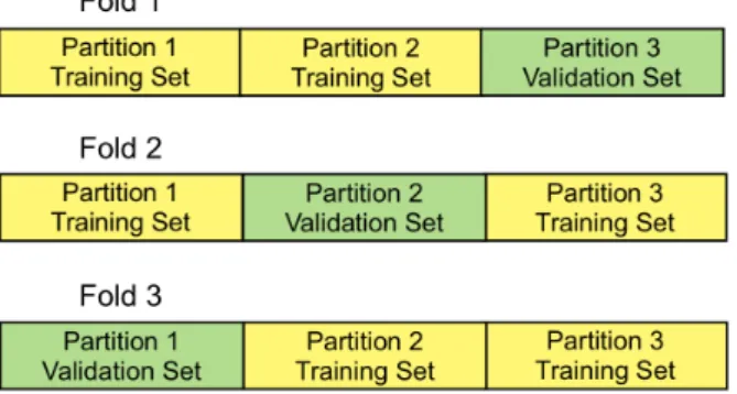
of the model’s predictive performance. There are several types of cross-validation methods such as leave-p-out, leave-one-out, and k-fold. Leave-p-out uses p observa-tions as the validation set and remaining as the training set, while leave-one-out is the special case when p= 1. At every iteration, the validation and training set are switched, and prediction results are gathered. K-fold cross-validation partitions the dataset intok equal parts, and uses 1 as the validation set and the remainingk−1as the training set, with each iteration changing them until all parts were used as vali-dation sets. There are some cases where the dataset may be unbalanced, containing more instances of one label than another, and splitting it may cause some labels to be absent. In stratified k-fold, the folds are created to preserve the proportion of classes of the original dataset.

Figure 1: A visual example of 3-fold cross-validation. The splits remain the same, but every iteration a different one is chosen as the validation set.

2.1.3 Data Representation and Feature Selection

Machine learning is a data-driven field, and the use of raw data has an important impact on the effectiveness of a model. Data sanitation and representation have an effect on the final results, sometimes even more than the particular machine learning method that is chosen. Data should be represented in such a way that commonalities and structures can be easily identified. This task may seem trivial but humans are sometimes not equipped with the tools to do it by manual examination, thus

(13)

we develop techniques on to obtain empirical data which can give insight on how representations and features affect the performance of an algorithm. The field of

feature engineering seeks to provide methods to automate the process of extracting the most relevant features from a given dataset. The benefits include facilitating data visualization and data understanding and reducing storage requirements, training and prediction times [GE03]. For big datasets, this can mean a difference of orders of magnitude when storing information and training a model.

An approach to selecting the most representative features is to find features that are highly correlated, meaning they share information, and only keep one to retain the information structure [Hal99]. Another popular method is principal component analysis (PCA) used as a dimensionality reduction analysis to find patterns in data of high dimensions which would otherwise be impossible to find manually. Lastly, there are techniques that take observed variables and combine them into other variables, called latent variables, helping to reduce the dimensionality of data.

2.1.4 Performance Metrics

In order to accurately compare models and make a proper decision, standardized metrics must be used. The metrics also depend on what kind of problem we are solving, classification or regression. Due to the nature of continuous variables in regression problems, its metrics are focused on formulas comparing the difference amongst expected and obtained values such as the sum of squared errors, and usually output numerical values instead of percentages. On the other hand, classification performance metrics have a discrete nature and they consider errors versus successes obtained in the predictions. This study is on a binary classification problem (spam detection) where prediction results are either true or false, and we focus on metrics for these kinds of problems.

There is no single classifier that works on all given problems, and selecting the best classifier may depend on what kind of performance is to be maximized. Popular metrics used to evaluate the quality of a classifier include accuracy, precision, and recall, and they represent ratios between expected and predicted results. In order to define these metrics, let us introduce several terms (in the context of binary classification) that describe classification results. Let P and N be the number of real positive and negative cases, respectively. We define T P as the number of true positives andT N as the number of true negatives the classifier returned;F P andF N

(14)

represents spam messages while the negative represents ham. The most commonly used metric is accuracy, which outputs the percentage of correct predictions using the formula

Accuracy= T P +T N

P +N .

Two other important metrics are recall and precision which formulas are

Recall= T P

P

and

Precision= T P

T P +F P.

Recall represents how many positive instances the model was able to classify, while precision gives the percentage of positive predictions that were correct. Specificity and Negative Predictive Rate (NPR) are the negative counterparts of recall and precision, represented by the formulas

Specificity= T N

N

and

Negative Predictive Rate= T N

T N+F N.

In the academic field, recall and precision are the terms often used and people are familiarized with the concept, so for clarity purposes, we will refer to specificity as ham recall and NPR as ham recall. There are datasets or problem domains where the data is not balanced (such as the one in this study) meaning there are more instances of a certain class than the other. Blindly maximizing accuracy in these cases may be misleading. To illustrate the problem, let us consider a dataset composed of 90%

false labels. If we run a dummy classifier that labels every instance asfalse, we can claim to have an accuracy of 90% and specificity of 100%. Nevertheless, looking at the precision score, it is equal to 0% (or NaN, given we have 0 true predictions). An alternative metric called balanced accuracy [UM15] addresses this problem by calculating the arithmetic average of recall and specificity with the formula

balanced accuracy= recall+specif icity

2 .

Taking the results of our dummy classifier above, the balanced accuracy is 50%, showing it is doing poorly on identifying one of the labels. Another metric which

(15)

helps us with unbalanced datasets is the F1-score which takes the harmonic average of precision and recall with the formula

F1-score= 2· precision·recall

precision+recall.

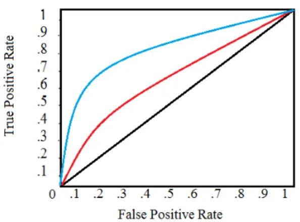
F1-score balances between precision and recall, since a classifier may be good at retrieving a certain class (high recall), but it does so by overcompensating and making mistakes in the labeling (low precision). F1-score gives equal importance to how many instances are correctly classified as well as how precise the classification is. The Receiver Operating Characteristic (ROC) curve is also used to evaluate the tradeoffs between true positive and false positive rates of the classifiers. The ROC curve is a plot of the recall against the false positive rate or fall-out calculated with

FPR= 1−specif icity.

Using this plot, we can see how the increase of the true positive rate relates to the false positive rate, assuring the model is not labeling everything as true to reach a better performance. Calculating the area under the curve (AUROC), we can obtain a score from 0 to 1 which summarizes the performance of a model in the ROC, with 1 being a perfect classification.

Figure 2: A ROC curve of two methods, and the diagonal marking chance perfor-mance (0.5). The AUROC score of the blue line is higher than the red line, thus making it a better classification method.

(16)

2.2 Text Classification

Since the World Wide Web was invented and once its first user-friendly interfaces appeared, information started to be generated and stored in massive amounts. With the addition of digital libraries, corporate databases, and email, we find ourselves surrounded by an enormous bulk of text-based documents for which analysis and/or classification can provide very useful information to its owners and users. Text clas-sification is a field of machine learning that seeks to classify documents or pieces of text into categories or clusters by a similarity score. It is relevant to several prob-lem domains such as spam filtering, language identification, sentiment analysis, and others. Until the late 1980s, the community in text classification was mainly looking at knowledge engineering for possible solutions; this approach required knowledge experts in the particular corpora to design a set of rules in a program that will be used as parameters of classification [SBF98]. The design and implementation of these systems were often done by pairings of domain experts and researchers, who would work in conjunction to digitize knowledge and incorporate it into a business or research platform. Knowledge engineering was useful in solving a particular problem domain, and its systems were constrained to the rules they were programmed with, and thus could only be improved with human intervention and knowledge. After a decade, and due to the clear limitations of this approach, the community began focusing on machine learning methods to develop algorithms capable of classifying text using a set of pre-classified documents to learn characteristics which can then be used for future classifications. These methods no longer relied on domain-specific, man-made rules, thus they could be used by other problem sets without structural changes. Algorithms, such as the Naive Bayes, SVM, and Neural Networks, are ex-amples of these methods where no expert knowledge is required. Some of them are capable of performing as good or better than knowledge-engineered tools, even with small or complicated training sets. Take for example Koller et al. [KS97], where they implemented a hierarchical multi-topic document classifier that used as little as 10 features to achieve close to85%accuracy. Other examples include Yu et al. [YX08], where achieved accuracy of95%using Naive Bayes and SVMs when detecting email spam from a corpus of 6000; or in Boiy et al. [BM09], where they succeeded to identify positive, negative and neutral sentiment in a multilingual set of documents with 83% accuracy.

With the community steering in the direction of machine learning, subfields have emerged within text classification. For example, feature engineering deals with the

(17)

fact that documents can be represented not only as abag-of-words(word counts), but also in alternative ways such as phrase extraction, hypernym extraction (word re-lationship) and word n-grams [SM99]. Phrase-based representation attempts to use the information that groups of words have by taking relevant slices containing two or more words and converting them into features. Hypernym-based representation takes advantage of the semantic information that words contain using hypernymy (a linguistic term for the “is a” relationship), thus it can extract more relevant meta in-formation about the meaning of the text. An N-gram is an N-character (or N-word) slice of a longer string, for example, “foo” is a 3-gram of “food”. N-gram-based repre-sentation groups words in their respective n-grams and derives the feature counting on these groups rather than exact matches. By representing documents in a different manner, these approaches seek to identify traits in the instances that could yield more meaningful information to the learning model, improving accuracy and overall performance by reducing the number of features. This advantage comes with the cost of a longer feature extraction step as opposed to calculating term frequencies in the bag-of-words representation.

Another important and closely related field to text classification is data mining. It is the process of discovering patterns in datasets without any previous knowledge, where the patterns provide further insight into the dataset, such as anomalies or dependencies [HMS06]. The results can even be used as a supplement to machine learning methods by identifying classes or groups not previously detected [FP96]. Data mining is considered a form of unsupervised machine learning with applica-tions such as categorization, DNA sequence mining, learning engineering and traffic analysis.

We now proceed to define the problem of text classification. Given a set of training documents D = X1, ..., Xn such that each document is labeled with a class value from a given set of classesC = 1, ..., k, and given an unknown document W, predict the label or class forW [AZ12]. The training documents are used to identify common features within the classes, making it possible to extrapolate these commonalities to future predictions. The classification problem assumes discrete values for the labels; in the case of continuous labels, it is called regression modeling. In problems such as multilabel classification, the documents can belong to multiple classes, whereas in binary classification, the documents can only belong to one of two classes. Spam classification is a binary classification problem with several applications such as:

(18)

labeling of its articles so the users can easily filter for specific topics. Given the volume of articles produced every day, machine learning models can be trained to label them, saving massive amounts of manual effort.

• Sentiment Analysis. In any given review website, there is always a metric which rates a given service or product, but beyond that, companies cannot tell what specific features of the service or product the users like or dislike. By doing sentiment analysis, these highlights can be extracted and a recommender can be trained to take into account features that users may like based on their past reviews.

• Email Routing. Most recent email inboxes have implemented different fold-ers or categories where they store incoming messages. Categories such as Trips, Purchases, Updates, and Finance help the user navigate and can be seen in Google Inbox, which has a built-in categorization of emails.

• Spam Detection. Undesired and potentially harmful messages are sent daily through several channels, email, text messages and instant messages are some examples. Apart from causing cluttered inboxes, these messages are frequently looking to scam the user of money or personal information, so it is on both the end-user and the company interest to detect and avoid such messages.

2.2.1 Spam Classification

A few ways of identifying spam include whitelists, blacklists, content-based, and any combination of the three. Whitelists and blacklists approach the problem by relying on identifying benign or malign senders to allow/stop incoming messages. This approach may prove effective to some extent, but once senders change their phone number or sender code, these solutions start to struggle. In this paper we approach the problem of spam classification from a content-based view, that is, using information in the text message itself to determine if it is desired or undesired. It is important to note that whitelists and blacklists can be built using content-based solutions and vice-versa.

In the field of machine learning, text classification may deal with multi-class prob-lems, i.e. sets of documents that can be classified into different categories that may or may not be mutually exclusive; spam classification only cares about two classes: spam or ham. Spam can be encountered in places such as blogs, email, social net-works, and forums. It can contain harmless (but unsolicited) information such as

(19)

marketing campaigns, but it can also form a part of a phishing or malware attack, potentially harming the recipient. One of the first studies was done by Sahami et al. who focused on using the Naive Bayes model as their classifier of email spam [SDHH98]. Making use of domain-specific properties, such as the sender informa-tion and the appearance of a manually curated list of words, they achieved close to perfect precision using a corpus of size 1789.

2.2.2 SMS Spam Classification

One of the first studies on SMS spam detection was presented by Almeida et al. [AHY11]. They introduce an SMS spam collection gathered from different sources including Grumbletext Website [Una], the NUS SMS Corpus [Kan11], Caroline Tag’s PhD Thesis [Tag09] and SMS Spam Corpus v.0.1 Big [HS11]. This SMS collection is used in our study. It is composed of4827legitimate messages and747 spam mes-sages. Apart from doing an analysis on the frequency and informational gain (IG) of the tokens in the dataset, they performed a duplicate analysis using plagiarism detection techniques to avoid adding similar (yet not identical) messages to their collection. This is a useful technique to be considered when building your own SMS collection. Using this newly constructed dataset, they compared two tokenizers and machine learning models to see which combination would yield the best results. The models included Naive Bayes (and several of its variants), SVMs, MDL, kNN, C4.5, and PART.

Shirani-Mehr [SM13] made use of the SMS Spam Collection v.1 [AHY11] to compare several machine learning models and their results. While no word stemming or misspelling fixes are done with the message instances, spaces, commas, dots or any other special characters are removed during the tokenization step. Also, the most and least frequent tokens found are removed from the dictionary, since they provide no additional information about a message. This is a common practice given that very frequent words can be found in the majority of the messages and rare words may cause the model to overfit based on them. Three additional features, number of dollar signs ($), number of numeric strings and overall message length were also included. Given all these features used, he found that message length has the highest mutual information (MI) of all, meaning it is an especially useful feature to use while classifying. Naive Bayes, SVM, k-NN, Random Forests, and Adaboost were all compared to find the best performing model. Naive Bayes was found to have the best accuracy and recall, even when increasing the complexity of the other

(20)

algorithms.

Given that SMS spam detection uses text classification algorithms, it is a very similar problem to email spam detection. The main difference is the fixed length of SMSs. Narayan and Saxena make use of existing email classification techniques in SMS spam detection to test their effectiveness [NS13]. They recognize various challenges stemming from the 160 character limit, including the use of acronyms and abbreviations, special treatment of bigrams and trigrams and overfitting of the model due to a limited corpus. The first experiment presented made use of a Bayesian email classifier with different tokenization methods (naive word split, email-like lemmatizer, n-grams). Using n-grams had the largest accuracy increase with respect to naive word split, but by only 7%. This shows that having complicated tokenizers such lemmatizers can hurt the performance of the classifier. It was also shown that the accuracy of this classifier was not comparable when using it for actual email. They then proceed to describe an improved approach at classifying short text messages using multi-level stacked classifiers. The process is as follows: the first-level Bayesian classifier records a subset of words whose individual probability is higher than a threshold, then this subset becomes the input of another model. If the probability does not meet the threshold, the instance is labeled as ham. Their results show that an SVM on two-level Bayesian classifiers yield the best accuracy of 98.8%, compared to single Bayesian (92.1%) and single SVM (93.9%).

Making use of the well known bag-of-words approach, which represents a text mes-sage by the occurrence of its words against a dictionary, Warade et al. study the results of doing feature selection by two methods: chi-square (CHI2) and informa-tion gain (IG) [WTS13]. CHI2 measures the independence between two variables, in this case, a feature and a label. The aim is to find features that are highly dependent on a label and discard those that are independent. IG measures the impact in the entropy of removing or adding a feature to the feature set in the performance of a classifier. Besides feature selection, input sanitization is performed to overcome intentionally misspelled words used by spammers such as “m0ney” for “money” or “off3r” for “offer”. This is called poison removal, and it is done by dividing the words into substrings of two characters and comparing them to a similar dictionary to find matches. Poison removal increases the overall accuracy of classification. Making use of Naive Bayes classifier, the two feature selection methods are compared. They discovered that the best result for both techniques is obtained when using the top 20 scoring features, with close to 90%. This is a suboptimal result considering the amount of preprocessing that was done.

(21)

Most of the previous work on SMS spam detection has been using content-based features, meaning using only information gathered from the text itself. Qian Xu et al.

take a different approach and make use of non-content features such as sender and recipient as well as the network information and metadata of the message [XXY+_12]. They divide such features into three categories: static, temporal and network-related. Static features include the total number of messages sent and the total size of the messages. Temporal features are the average sending time, number of messages during a day and number of recipients in a day. Lastly, network-related features include the total number of recipients and the clustering coefficient describ-ing how a sender is connected to its recipients. An SVM is chosen as the learndescrib-ing model after an initial comparison with kNN. They perform experiments using only one category of features and all three at the same time. The results show that using all three categories results in almost the same improvement as only using temporal and network features alone. Using PCA, they extract the most important features with number one being the total size of messages, the next eleven being temporal features, tailed by a network feature.

While extensive work has been done using supervised machine learning methods for SMS spam detection, they all have the weakness that a sufficiently large and reliable training corpus is required. The unsupervised or semi-supervised counterparts have not had great attention, but Gianella et al. employ character n-gram counts to de-velop a semi-supervised algorithm, capable of reaching high accuracy scores with a small training set. This technique was based on an email spam detection procedure developed by Uemura et al. [UIKA11] which assumes ham messages tend to contain more complex content than the spam messages. Using an extension of the model in Resnik et al. [RH10] as their probabilistic generative model, they estimate its pa-rameters from unlabeled and labeled data. They found that their unsupervised and semi-supervised models outperformed other supervised models such as Semiboost and SVM when the training set was small and performed comparably when the training set was larger. Further on, active and transfer learning can also address the issue of the limited number of training sets available. For example, transfer learning attempts to reduce the size of the required training set by employing trained models from a different domain, such as email spam, to improve the results of a model only using SMS corpus alone.

(22)

3 Classification Models

In this section, we review the machine learning methods used in this study: Naive Bayes, Support Vector Machines and Neural Networks. We present an overview of each algorithm and any previous relevant research on spam detection.

3.1 Naive Bayes

Naive Bayes is a type of machine learning algorithm that uses Bayes’ theorem and assumes conditional independence between the features. While this assumption is false in most cases, the model can still perform difficult classification tasks very well and sometimes better than more complex models. Bayes’ theorem estimates the probability of an event based on prior knowledge of conditions in which said event occurred [Rou18]. Naive Bayes has been a popular machine learning algorithm for many years due to its simplicity and acceptable performance and a lot of research has been done to address its weaknesses. While it can provide classification probabilities, these are not very accurate, and people often use it as a classifier where the class with the highest probability is chosen. The application of the Naive Bayes classifier to spam filtering was initially proposed by Sahami et al. [SDHH98] who used it as a decision framework. It was proven to be an effective model without much manual tuning with a precision of97%and a recall of94%using only words as features. They also studied how accurate the model was when also adding hand-picked features such as the presence of “spammy” words like FREE, (!!!), or $$$, reaching close to perfect scores with their testing set. With its lack of complexity, Naive Bayes has been proven to be an effective model in text classification and it has become one of the preferred methods used in spam classification.

Rennie et al. [RSTK03] list several systemic problems in the Naive Bayes classifier. One problem is that the model performs poorly with an unbalanced training set (occurrences of one class are higher than the other). Another problem is that the conditional independence assumption ignores completely the evidence of a relation between two or more words. They also argue that multinomial Naive Bayes does not model text well and propose using inverse document frequency (idf) which gives greater weight to words with rare occurrences. They provide experimental results that show that their three improvements to Naive Bayes result in better performance of the algorithm.

(23)

and Bernoulli. Given the nature of text classification, the type used in this study is Multinomial Naive Bayes. McCallum et al. [MN+98] found that Multinomial Naive Bayes performed better than other models at text classification even with a small training set, and one could reduce its error significantly by increasing its vocabulary size, although this increase is not linear.

3.1.1 Multinomial Naive Bayes

Multinomial Naive Bayes (MNB) is the defacto Naive Bayes algorithm used in text classification since it is the most suitable to represent a document. In the multino-mial model, a document is represented as a vector of counts of events, where each count is the number of times a word from the gathered vocabulary appears in the document. This is what is known as the bag-of-words or term frequency represen-tation. The naive assumption is that the appearance of a word is independent of the other words in the same document. Making use of the prior parameters of each class, we can estimate the posterior probability given the evidence (our bag-of-words representation), by multiplying the probability of each word in the document and selecting the class with the highest probability (ham or spam). One of the main critiques of the Multinomial Naive Bayes is that it completely ignores the order that words occur in a document, although this is part of the independence of features assumption.

Let us describe MNB in more detail by analyzing the formulas and rules it is based on. Let C be a set of classes, let N be the size of our corpus or vocabulary. MNB assigns a test document d to the class c that has the highest posterior probability

P(c|d) defined by Bayes’ theorem as

P(c|d) = P(c)P(d|c)

P(d) ,

where P(c)is the class prior calculated by dividing the number of documents with class cby the total number of documentsC. P(d|c)is called the likelihood and it is the probability that we see documentd in classc. Using the chain rule to calculate the likelihood, we expand it as

P(d|c) =P(t1|t2, ..., tn, c)P(t2|t3, ..., tn, c)...P(tn−1|tn, c)P(c),

(24)

term ti is conditionally independent of every other term, then we can rewrite it as

P(t1|t2, ..., tn, c) =P(t1|c). Thus, the likelihood formula is reduced to

P(d|c) =P(c) n Y

i=1

P(ti|c),

where P(ti|c) is the probability that term ti appears given class c. It is estimated with P(ti|c) = a+P d∈Dcntid b+P t0 P d∈Dcnt0d ,

where Dc is all the documents of class c, t0 is all the terms and the denominator returns the count of all words in all documents of classc. a andb are the correcting terms which are used so P(ti|c) does not equal to zero in the case that ti does not exist in the corpus. This is important otherwise our likelihood formula above,P(d|c), will automatically be zero if one of the terms is not in the corpus. When we choose

a = 1 and b = N, it is called Laplace smoothing, which assigns an initial count of 1 to every term, and normalizes their probabilities by dividing by our dictionary size, N. The formula can be viewed as a division of counts, the numerator being the number of timesti appears in documents of classc, divided by the total number of words in documents of class c. It is the proportion that a word takes in the subdictionary of classc.

As mentioned before, Naive Bayes and its variants are generally not used to cal-culate the exact posterior probability but only to obtain the class with the highest probability; this lets us ignore the P(t) in the denominator and only calculate the likelihoods for all classes and take the highest value. We can express this classifier that assigns a classc toyˆwith the formula

ˆ y= arg max c∈C P(c) n Y i=1 P(ti|c).

Kibriya et al. [KFPH04] claim that all the Multinomial Naive Bayes modifications presented in Rennie et al. [RSTK03] are not necessary and that by only transform-ing the word counts ustransform-ing term frequency inverse document frequency (TF-IDF)

(25)

yields improved results without much complexity and extra calculations. TF-IDF comes from the multiplication of term frequency(TF) and inverse document fre-quency (IDF), hence its name. Its formula is

TF-IDF(word, D) = log (f + 1) logD

df,

wheref represents the frequency ofword,Dis the total number of documents in the corpus anddf the number of documentswordappears in. It is a numerical statistic used in information retrieval to reflect how relevant a word is to a document in a collection of documents. Its value increases with the number of appearances of the word in the document and is reduced by the frequency of the word in the corpus. If instead of term frequencies, TF-IDF is used in MNB, the likelihood formula for a term ti given class cwould change to be

P(ti|c) = P d∈DcTF-IDF(ti, d) P t0 P d∈DcTF-IDF(t 0_{, d}₎.

A termti which appears several times solely in classcdocuments will return a higher score since it is taken as more representative of class c. In Section 6, we perform our own experiments of MNB versus a TF-IDF MNB.

3.2 Support Vector Machines

Support Vector Machines (SVMs) are a group of supervised machine learning al-gorithms commonly used for classification problems but also used for regression. They were first introduced as a learning algorithm for binary classification problems [CV95] and then extended to multiclass classification and regression [G+_{98]. Their} core idea is to separate instances into two classes by finding a hyperplane which maximizes the distance from each group of instances. They were conceived for lin-early separable binary problems and extended to nonlinlin-early separable problems with the use of the kernel trick. Kernel functions allow algorithms to operate in high-dimensionality domains by being able to compute a similarity score between two feature vectors. They are highly accurate and work well with small training sets. Their main weakness is their training time can be slow (even if the number of features is low), making it non-ideal for larger datasets classification. They do not provide probabilistic estimates although these are not needed for the classifica-tion problem in this study. Since SVMs attempt to split the classes in the given

(26)

dimensional space, they are hardly affected by unbalanced training sets.

In one of the first experimental studies of SVMs, Chapelle et al. [CHV99] used a dataset with 14 categories each with 100 images for a total of 1400 images, repre-senting them by mapping their pixels to a histogram which can easily be used by an SVM. After experimenting with various kernel types and parameters, their results show that error rates as low as 11% could be achieved. While this may seem a high error rate, it should be noted that there were 14 categories with not many instances, confirming the claim that SVMs perform well with small datasets.

Within the field of text classification, Kwok experiments with SVMs using news stories classified around 135 financial topics [Kwo98]. As a preprocessing step, he applied inflectional stemming, stop word removal, conversion to lowercase and elim-ination of words which appeared in less than 3 documents. He coded the resulting documents using the TF-IDF representation. The performance was measured by recall and precision and compared to kNN. While the SVM results were favorable, the difference was not outstanding, but the advantage that SVMs have over the kNN algorithm is their ability to take in new training instances fast and without taking much memory.

In a more related study, Drucker et al. [DWV99] approach the spam classification problem with SVMs. Using different feature representations like term frequency and binary and comparing to other classification algorithms like boost and decision trees, they find low error rates of 5% and better performance times. A particularly interesting find was that converting words to lowercase yielded more accurate results, which makes sense since this normalizes the data across the set.

3.2.1 Kernels

SVMs need a similarity measure that is used to compare instances to each other and find the separating hyperplane. A kernel is a function that takes two vectors and returns a measure on how similar they are to each other. The most basic kernel used is the dot product or linear kernel calculated by the dot product where the vectors represent two instances and their features. The dot product is sensible to the magnitude of the vectors, thus it is important to normalize the input vectors, otherwise feature vectors with higher magnitude will produce a higher dot product than their lower magnitude counterparts.

(27)

instance set and number of features are large for better computational performance. In our use case, the number of instances is high due to the traffic and our training set, and speed is of high importance, so we can sacrifice some accuracy for a faster SVM.

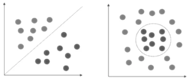
There are problems where the data cannot be correctly separated using a linear kernel since it is nonlinearly separable. Take for example Figure 3 where the left dataset can be linearly separated and the right side requires a more complex function.

Figure 3: Two different datasets, linearly and nonlinearly separable respectively.

Given that the dataset is to be split using a hyperplane, a nonlinearly separable problem can be remapped onto a different dimensionality space using a different kernel. Expanding on the linear kernel, we also have thepolynomial kernel calculated as

k(x, w) = (x·w+b)d,

where b is the intercept coefficient and d is the degree of the kernel. To better illustrate how polynomial kernels overcome the obstacle of nonlinearly separable datasets, let us look at Figure 4 where we have a one-dimensional dataset which can be easily separated. Then, in Figure 5, we see another dataset with the same dimensionality but it cannot be separated. Lastly, using a 2-degree polynomial kernel, we see in Figure 6 that now a hyperplane can be obtained to correctly separate this dataset.

(28)

Figure 4: A one-dimension linearly separable dataset.

Figure 5: A one-dimension nonlinearly separable dataset.

Figure 6: The same dataset of Figure 5 but mapped into a 2-dimensional space using a 2-degree polynomial kernel. Note that the dataset becomes linearly separable after the kernel is used.

There are still cases where even a high-degree polynomial kernel function may not suffice to accurately classify a dataset. These datasets are often addressed by using the Radial Basis Function orRBF kernel, which calculates the distance between two vectors with the formula

RBF(x, w) = exp (−||x−w||

2 2σ2 ).

One can recognize ||x−w||2 _{as the Euclidean distance between two vectors.} 1 2σ2 is

(29)

commonly referred to as theγ parameter, which simplifies the formula to

RBF(x, w) = exp (−γ||x−w||2₎_.

We end up with a decaying function where the closer the vectors are to each other, the higher similarity score. In fact, this function is of the form of a bell-shaped curve and larger values ofγ yield narrower bell curves. In more general terms, theγ

parameter dictates how far the influence of a single training example reaches, with higher values having a smaller sphere of influence than lower values. A smallγ may cause overfitting since two instances need to be very close together to be considered similar. Conversely, a large γ may lead to high bias due to the relaxation on the similarity between two instances [VD04].

3.2.2 Separating Hyperplane

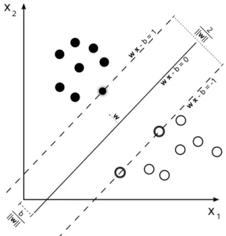
To better explain how an SVM creates the hyperplane separating a dataset, we take the linear kernel SVM as an example. This variation allows for faster computations due the simple calculations required by its similarity measure. The linear SVM as-sumes that there exists a hyperplane such that it completely separates the instances into two groups representing their classes. This hyperplane is created by maximizing the distance from the nearest point from each class. The hyperplane can be written as

w·x−b = 0,

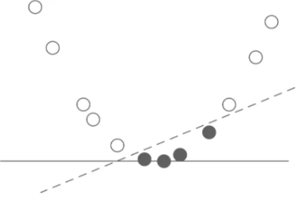
where w is the normal vector to the hyperplane, x is the slope of the hyperplane and b is an offset constant hyperparameter. Figure 7 illustrates how this function separates two classes of points and their corresponding margin functions, which are obtained by making the hyperplane function equals to1 and −1.

(30)

Figure 7: Illustration of how the hyperplane obtained by an SVM separates and classifies points with two different classes.

This approach assumes that the dataset is linearly separable, but in the case of nonlinearly separable problems, we introduce a hinge loss function that maximizes the margin by which the hyperplane separates each point, allowing for errors in classification but minimizing them. A hinge loss function is defined as

L(y) = max(0,1−ty),

whereyis the output of the hyperplane function andtis the intended output(−1,1) in a binary classifier. It can be seen that when both yand thave the same sign and

|y| ≥ 1, L(y) = 0. When their sign is different, the penalization increases linearly withy, and similarly, if the classification is correct but the margin of the prediction is not sufficient (|y|<1), there is still a penalty returned.

3.2.3 C parameter

Apart from the kernel selection and kernel parameters, SVMs have an additional parameter C which tells them how large is the penalty for misclassifying a training sample when calculating the separating hyperplane. Larger values of C cause the

(31)

SVM to find a hyperplane that separates all training samples correctly, which may lead to overfitting of the model. Smaller values ofCrelax this constraint by allowing more misclassifications in the training phase, which can be useful to preserve the generalization of a model but may also cause underfitting of the data. Experimenting with different values ofCis usually done using exponentially growing sequences such as10−4_,₁₀−2_{, ...,}₁₀4_.

3.3 Neural Networks

Neural Networks (NN) have been a popular topic in the last years, especially with the advent of Deep Learning. At the basic level, a NN consists of many simple interconnected units called neurons, and each of them produces real-valued activa-tions depending on the input given [Sch15]. Deep Learning methods aim at learning features by forming different levels and hierarchies of learning by the composition of lower levels. They are inspired by human cognition and how neurons interact with each other to form what it is conceived as human learning. While the first NN were being developed as early as the 1970s, Deep Learning started to become feasible since the early 2000s with the rise of more powerful hardware and the increase of data accumulation. With these advantages, they outperform kernel-based methods, such as SVMs, in complicated problems. Another reason for its rise in popularity was the ever-lowering computing cost and cheap parallel processing power, which NNs benefit greatly from due to their naturally parallel structure.

An NN text classifier is a network where each neuron receives the term frequencies (or any other feature representation) of a document as input and returns a real value representing the activation of the neurons that can be used to predict the category or class of the document. Each neuron has a set of term weights that are used to compute the activation function. A frequently used activation function is the linear activation function calculated with

pi =A·Xi,

where Xi contains the term frequencies of document i, and A the term weights in a neuron; note that both are the same length. Considering a binary classification problem, the sign of pi will represent the class of document i. Thus, the goal is to learn the correct weight values ofAwith the use of training data. A naive approach is to start with random weights and iteratively update them when a mistake is

(32)

found in the training phase. The update magnitude is called the learning rate (µ) and we stop once all training samples are correctly classified or we reach a maximum number of iterations. This is the core idea of the perceptron algorithm [Ros58]. A pseudocode implementation is presented in Algorithm 1.

Data: training documents X, training labelsy, learning rate µ

Initialize weight vectors A to0 or random real values converged← false

repeat

converged← true for Xi, yi ∈X, ydo

// Apply training data to the neural network

pi =A·Xi

if sgn(pi)6=yi then

// update weights A by learning rate µ

A=A+µ·yi·Xi converged← true end

end

until converged is false;

Algorithm 1: Perceptron pseudocode.

The perceptron is a linear classifier, thus it requires a linearly separable dataset, otherwise, it will not converge. If the problem is not linearly separable, there are several approaches that can be taken. One is to implement a pocket algorithm which wraps around the perceptron and keeps the best solution found so far by calculating the classification error of the weight vector in each iteration. If no optimal weights are calculated after k iterations, we return the pocketed solution. The pseudocode for the pocket algorithm is shown in Algorithm 2.

(33)

Data: training features X, training labelsy, learning rate µ, max iterations k

Result: weight vector Apocket

InitializeApocket to0 or random real values for i= 0...k do At=Apocket for Xi, yi ∈X, ydo pi =At·Xi At=At+µ·(yi−pi)·Xi end

if error(At)< error(Apocket)then Apocket =At

end

if error(Apocket == 0) then

break end end

Algorithm 2: Perceptron pseudocode with a pocket implementation.

While the pocket version of the perceptron is guaranteed to return a solution, it may not be the optimal solution, rather the best found so far. Further variations address this caveat, like the Maxover algorithm [Wen95] which converges to a global optimal for separable data and to a local optimal in the case of non-separable data. The perceptron is an online algorithm, meaning the training is done piece-by-piece and does not need the entire training set from the start, making it capable of fitting new samples later on. This is particularly useful in cases where new labeled instances can be obtained after training. For example, an email classifier can be set up to organize a userś inbox, but also the user is continuously tagging emails so the model is updated according to this feedback.

The neuron can be thought of as the most basic unit in an NN while the perceptron is the algorithm the neurons perform for fitting. As mentioned before, the perceptron is suited for separable datasets, but the use of multiple layers of neurons can be used in order to create non-linear classification boundaries, producing the Neural Network. The effect of having multiple layers is to induce piecewise linear boundaries, which in the end approximate enclosing regions containing specific classes.

(34)

3.3.1 Multilayer Perceptron

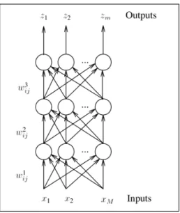
Pal et al. [PM92] describe the multilayer perceptron (MLP) as a network “consist-ing of multiple layers of simple, two-state, sigmoid process“consist-ing elements (nodes) or neurons that interact using weighted connections”. It is composed of a minimum of three layers: input, hidden and output layers and it may contain more than one hidden layer. There are no connections between neurons within a layer, but all nodes are connected with all nodes of neighboring layers, forming what is called a fully-connected network. The weights represent the correlation between activities happening across nodes in the layers. Figure 8 contains a graphical representation of a multilayer perceptron.

Figure 8: Multilayer Perceptron. Each node is connected to the other nodes in the adjacent layers. Their connection weights are represented bywl

ij whereiis the source node, j the destination node and l the layer. Inputs and outputs are represented by

xm and zm respectively.

3.3.2 Backpropagation

A typical way of training a NN is error backpropagation, in which the classification error is sent back to the network so the parameters can be adapted to reduce the error between the target output and the network output [Seb02]. To perform error

(35)

backpropagation we need a loss function that helps us evaluate how far apart are the results from the network with respect to the target results. This function is of the form f(yout, ytarget) and returns a real number depending on the magnitude of the difference between the two values. A commonly used loss function is the sum of squares function calculated with

loss(y_out,y_target) = |y_out−y_target|2_,

wherey_out is the predicted value calculated by the network andy_target is the correct output value we look for. There are a couple of reasons for using the sum of squares as a loss function. First, it does not matter if the network underestimates or over-estimates, the error will always be positive, so the goal is to reduce it or reach zero. Second, big errors in the network are more heavily penalized than small errors due to the squared value. If we would plot the obtained prediction value in the x-axis against the loss value in the y-axis, we would get a parabola (sum of squares). We can say that our objective is to “descend” the error parabola to find our desired weight value. To figure out if the weight should be decreased or increased for a smaller error, we use the partial derivative of the loss function with respect to the weights, as it tells us the rate of change at that given point. This is called the

gradient. Since we are minimizing the loss function, we follow the opposite direction of the gradient. This leads us to thelearning rate, which is a constant (usually very small) used to update the weights slowly and smoothly in the opposite direction of the gradient, in other words, towards a minimum error. The algorithm which per-forms this loss function minimization is called gradient descent and is widely used in machine learning along with other methods such as stochastic gradient descent,

AdaGrad and Adam [RM51, DHS11, KB14]. The backpropagation occurs after the

error is calculated at the output layers and its weights are updated; it is then passed back to the hidden layers where the gradient is obtained again but now with respect to their own weights, and the process is repeated until reaching the input layer. This is a simple and intuitive explanation of how error backpropagation works but the mathematical background behind it is more involved.

The strength of NN classifiers is that they can model the data very precisely, leading to high accuracy in the classification but it may also cause overfitting of the training data, so when using a large number of features, NNs may perform worse due to over-fitting. Schutze et al. [SHP95] design a NN which minimizes overfitting by having a validation dataset, one-third of the size of the training set. At every iteration, they

(36)

run the validation set to obtain its error rate, when this rate goes up, then it means the network is starting to overfit on the training data and they stop, resulting in a more generalized network. The overfitting problem in neural networks is a widely studied topic and extensive effort has been made on finding techniques that reduce variance. Some examples include cross-validation, early stopping, dropout, among others [MB90, CLG01, SHK+_14].

Clark et al. [CKP03] present of the first studies on spam classification using NN, which used a fully connected multilayer perceptron using 20 to 40 hidden layers and the validation set error as the early stop. They found that using TF-IDF as document representation yielded the best results and outperformed NB, kNN, and TreeBoost, with performances close to perfect in some datasets.

(37)

4 Data Set

Before going into the training of a model, the dataset used must be first transformed into a representation that is both accepted by the model and advantageous to its performance. The structure, the representation and, the information of the input data will strongly affect the performance of a classifier. As we have seen in Sections 2.2 and 2.2.1, the traditional representation of bag-of-words has proven superior to other more complex feature representations. Given that this approach is very fast both for training and prediction phases, we make use of it throughout the empirical part of this study except for the TF-IDF-based Multinomial Naive Bayes. Nevertheless, it is a potential aspect which can be analyzed in more detail for future studies.

We make use of two different datasets throughout the study. The first is the publicly available dataset by Almeida et al. [AHY11] which is composed of several collections:

• A collection of 425 spam messages from the Grumbletext website, where UK users report spam messages [Una]. Almeida et al. had to manually review the complaint reports to extract the actual message content, but this guarantees the data comes from real traffic and labeled by an end-user.

• A corpus of 3,375 ham messages of the NUS SMS Corpus, which is a dataset of over 10,000 legitimate messages gathered by the Department of Computer Science at the National University of Singapore, where the messages were obtained from volunteers [Kan11].

• 450 of ham messages from Caroline Tag’s PhD Thesis [Tag09].

• The SMS Spam Corpus v0.1 containing 1,002 ham messages and 322 spam messages [HS11]. This dataset has been used in other academic studies such as Scott et al. [SM99] and Cormack et al. [CGHS07].

Together, the collection contains 4,827 ham and 747 spam messages for a total of 5,574 messages. The messages were modified to protect the privacy of the users by changing names, addresses, and other personal information. The number of messages in this dataset allows us for enough room to test how training models with a different number of messages affect their performance.

The second dataset we use is gathered from the traffic of the Veoo platform. It is composed of 1,318 ham and 159 spam messages, which were also modified to

(38)

hide personal and sensitive information about the users. While a first iteration of the spam detection system was implemented using the dataset in Almeida et al. [AHY11] with favorable results, a dataset of the actual traffic was created so more controlled experiments can be made on the efficacy of training models using these two datasets, either together or separate.

4.1 Preprocessing

Datasets often contain pieces of information that may degrade the performance of a learning algorithm. There are several studies on text classification which make use of preprocessing techniques such as stop-word removal, tokenization, and word-stemming to eliminate or convert this data into more valuable information [SR03, LSTO10, CT94]. The preprocessing done was mainly to ensure that messages had a valid encoding and characters, and obscuring personal details, everything else was left as-is.

(39)

5 Platform Architecture

5.1 Company

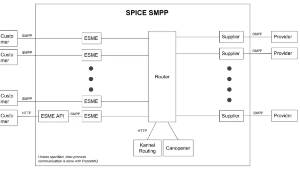
Veoo is a mobile solutions platform that enables businesses to deliver mobile ser-vices by simplifying technical, commercial and regulatory complexities. Businesses looking to implement mobile marketing campaigns, mobile payments, and other mobile-based services can employ Veoo’s processes without having to work through the difficulties of implementing their own messaging technology and having to worry about the regulations that different regions or countries may have. It offers differ-ent interfaces that allow clidiffer-ents from varying technical backgrounds to develop text messaging solutions. Specific examples of these interfaces are HTTP and the SMPP protocol. The SMPP (Short Message Peer to Peer) protocol was established and managed by the SMS Forum organization which provided a flexible solution for the sending and receiving of mobile short message data between external entities and message centers. The protocol supports several two-way messaging functions such as:

• Transmitting messages from an ESME (External Short Message Entity) to single or multiple destinations via an SMSC (Short Message Service Center).

• Querying the status of a short message.

• Canceling or replacing a short message.

• Defining the data coding of a message, examples of supported encoding include GSM, UTF-8, and Latin-1.

• Providing a service type to a message e.g. voicemail notification, cellular paging.

SMSCs commonly require third-parties to communicate with them using this pro-tocol, and due to some nuances in the propro-tocol, it is not unusual to see different implementations that may be incompatible with each other. Veoo offers its users a transparent SMPP connection to several SMSCs without having to deal with the differences between their protocols.