The Impact of Probabilistic Classifiers on Appointment Scheduling with No-Shows

AIS Electronic Library (AISeL)

AIS Electronic Library (AISeL)

ICIS 2019 Proceedings

IS in Healthcare

The Impact of Probabilistic Classifiers on Appointment

The Impact of Probabilistic Classifiers on Appointment

Scheduling with No-Shows

Scheduling with No-Shows

Michele Samorani

Santa Clara University, [email protected]

Shannon Harris

Virginia Commonwealth University, [email protected]

Follow this and additional works at: https://aisel.aisnet.org/icis2019

Samorani, Michele and Harris, Shannon, "The Impact of Probabilistic Classifiers on Appointment Scheduling with No-Shows" (2019). ICIS 2019 Proceedings. 7.

https://aisel.aisnet.org/icis2019/is_health/is_health/7

This material is brought to you by the International Conference on Information Systems (ICIS) at AIS Electronic Library (AISeL). It has been accepted for inclusion in ICIS 2019 Proceedings by an authorized administrator of AIS Electronic Library (AISeL). For more information, please contact [email protected].

The Impact of Probabilistic Classifiers on

Appointment Scheduling with No-Shows

Completed Research Paper

Michele Samorani

Santa Clara University

Santa Clara, CA 95053, USA

[email protected]

Shannon Harris

Virginia Commonwealth University

Richmond, VA 23284, USA

[email protected]

Abstract

Appointment no-shows are common in outpatient clinics and increase clinic costs and

patients’ dissatisfaction. We develop a framework to predict the no-show probabilities of a given set of patients, and to subsequently employ these predictions to find the optimal appointment schedule. Some existing work assumes that all patients have the same no-show probability (1-class approach); other work assumes that patients have either a low or a high no-show probability (2-class approach). In contrast, we utilize probabilistic

classifiers to obtain the individual patients’ no-show probabilities (N-class approach). Our approach results in better-quality schedules, as measured by a weighted average of patient waiting time and provider overtime. We also find that a small increase in the prediction performance (measured by the Brier score) translates into a large decrease in the schedule cost. Our results are obtained through a large-scale computational study and validated on a real-world data set from an outpatient clinic.

Keywords: IS in Health Care, Appointment No-Shows predictions, Appointment Scheduling with No-Shows

Introduction

Appointment no-shows occur when patients fail to show up for their clinic appointments. No-shows are

common in many outpatient clinics, and increase clinic costs and patients’ dissatisfaction. No-show rates in primary care clinics have been found to range from 12% to 30% (Whittle et al. 2008, Goffman et al. 2017). For fiscal year 2008, the Veterans Health Administration (VHA) reported an 18% no show rate, and estimated the total cost of no-shows at $564 million annually (U.S Dept of Veterans Affairs, OIG 2008). In order to mitigate the negative effects of no-shows, a clinic may implement open access (OA) scheduling, where patients are assigned appointments times in the near future, typically at most two days in the future. Liu et al., 2010 study scheduling of patients to outpatient appointments in an OA setting, and find that OA is typically best when the supply of appointments is similar to appointment demand. In lieu of this, a common way to counteract no-shows is to overbook appointment slots, a practice where more than one patient is assigned to an appointment slot. Overbooking may cause the clinic to be overcrowded, which in turn may result in patient waiting time and provider overtime. A patient experiences waiting time whenever their appointment cannot start at the predefined appointment time because the provider is seeing another patient; the provider experiences overtime when there are patients waiting to be seen at the end of the clinic session. The former effect increases customer dissatisfaction while the latter effect increases the clinic costs.

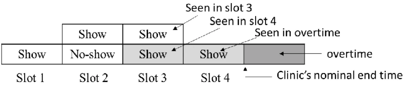
Figure 1 illustrates an example where six patients are scheduled in four slots (i.e., slots 2 and 3 are double-booked) and one of the patients scheduled in slot 2 does not show up. Assuming that the provider can only see one patient per appointment slot, there will be two patients (highlighted in light grey) who will have to wait for the length of one appointment slot beyond their scheduled time (i.e., they will incur one time unit of waiting time); because the last scheduled patient will be seen after the end of slot 4 (i.e., the clinic nominal end time), the provider will incur one time unit of overtime.

Empirical evidence suggests that a patient’s no-show probability is correlated to certain appointment and

patient characteristics like the patient’s age, gender, and prior no-show history, or the appointment lead time (i.e., the time between when an appointment is made and when it is to occur) (Galluci et al. 2005, Goffman et al. 2017, Harris et al. 2016, Whittle et al. 2008). Despite this, most outpatient clinics do not attempt to estimate the individual no-show probabilities to inform scheduling decisions; instead, clinics typically build their schedules under the assumption that all patients have the same no-show probability.

Figure 1: An example of schedule where two patients experience waiting time (light-grey) and the provider experiences overtime (dark-grey)

In this paper, we introduce an integrated framework to predict no-shows at the individual appointment request level, and to subsequently employ these predictions to find the optimal appointment schedule, that is, the schedule that minimizes a weighted sum of the expected patient waiting time and provider overtime. The input of our framework is a set of appointment requests. The output is a schedule, that is, an assignment of each appointment request to an appointment slot, such that each patient is assigned to a slot, but each slot may be assigned to multiple patients. Our framework has two main components: the first is a probabilistic classifier that estimates the no-show probabilities of a set of appointment requests; a probabilistic classifier is a predictive model capable of providing not only a binary prediction (i.e., no-show versus show), but also the no-show probability for each input observation. The second component is a stochastic mixed integer program that schedules the 𝑁 appointment requests in 𝐹 slots (with 𝐹 < 𝑁) given

the appointment requests’ estimated no-show probabilities. The research questions that we address are:

1. How can individual no-show probabilities be effectively employed to optimally schedule appointments? 2. How can a classifier be selected to predict individual no-show probabilities?

Both research questions have largely been neglected by the existing body of work. Regarding the first question, most research in data-driven appointment scheduling assumes that all appointment requests have the same no-show probability (i.e., 1-class approach), typically equal to the population no-show rate. Other work assumes that appointment requests have either a low or a high no-show probability (i.e., 2-class approach). In contrast, this work considers any number of classes, up to the case where each appointment request has its own no-show probability (i.e., the 𝑁-class approach).

Regarding the second research question, the majority of the existing work has focused on finding the classification technique that maximizes the Area under the Receiver Operating Curve (AUC). This choice may at first sound sensible, because (1) maximizing the AUC is the preferred metric for binary classification on imbalanced data sets and (2) predicting no-shows is an imbalanced classification problem, since the majority of patients is expected to show. However, we find that the classifier with the largest AUC is not necessarily the one that leads to lower-cost schedules. In fact, our preliminary results suggest that the

Brier’s score – a metric used to evaluate the quality of predicted probabilities– may be a more suitable metric to use when selecting a classifier.

The two main contributions of our work are as follows. First, to the best of our knowledge, our work is the first to develop an optimal solution method to schedule outpatient clinic appointments given individual patient no-show probabilities. Second, we show that our method obtains higher-quality schedules – as measured by the schedule that minimizes a weighted sum of the expected patient waiting time and provider overtime – than the typical 1-class and 2-class approaches.

In addition to obtaining higher-quality schedules, we performed a preliminary study to help uncover two managerial insights which may be very valuable in designing prediction-based appointment scheduling systems. First, we show that selecting the classifier with minimum Brier’s score on the calibration set, as opposed to the one with maximum AUC, may result in higher-quality schedules when considering appointment requests from the test set. Second, our preliminary results suggest that even a marginal

decrease in Brier’s score (e.g., 0.20 to 0.19) may translate into a significant cost saving (e.g., 15%), as measured by the resulting schedule cost. These findings suggest that organizations should spend significant resources to maximize the prediction performance of their probabilistic classifier.

Our results are obtained through a large-scale computational study and validated through real-world data from a local outpatient primary care clinic.

Literature Review

Our paper contributes to Information Systems (IS) research in the form of machine learning and optimization methodologies that improve operational efficiency of outpatient clinics. In this sense, our research falls under the IS field of Computational View of Technology, as categorized by Orlikowski and Iacono (2001).

Our work draws from and contributes to two distinct areas of research. The first area is composed of empirical papers that study the factors related to appointment no-shows. Papers have found factors such as past no-show history (Harris et al. 2016, Goffman et al. 2017, Whittle et al. 2008), lead time, age, and gender (Gallucci et al. 2005, Goffman et al., 2017, Partin et al. 2016, Whittle et al. 2008) to be correlated with no-shows. Because the focus of these papers is to describe the factors that are related to no-shows, they typically do not discuss how the resulting probabilities may be integrated into a clinic schedule. Additionally, the metric used to measure predictive performance is typically the AUC. Daggy et al. (2010), Srinivas & Ravindran (2018), and Samorani and LaGanga (2015) discuss both no-show prediction and the resulting schedule in their papers, but they do not employ no-show probabilities at the individual patient level. In contrast, we discuss both no-show prediction and the resulting schedule while incorporating individual no-show predictions, and show that choosing a classifier based upon minimizing the Brier score results in a better quality schedule as opposed to maximizing AUC.

The second area of research that our paper contributes to is appointment scheduling. The papers published in this area aim at optimally scheduling appointment requests in order to minimize a weighted sum of patient waiting time and provider overtime. Most of the works in this area employ a 1-class approach, where each appointment request is assigned the same no-show probability, which can be readily obtained by

computing the population’s historical no-show rate (LaGanga & Lawrence 2007, LaGanga & Lawrence 2012, Robinson & Chen 2010). Some more recent works implement a 2-class approach, where patients are split into two classes of no-show probabilities (Zacharias & Pinedo 2014, Liu et al. 2010, Srinivas & Ravindran 2018). To the best of our knowledge, only Zacharias & Pinedo 2014 extend the 2-class approach to a N-class approach, where each patient’s individual no-show probability is utilized. However, Zacharias and Pinedo (2014) provide only analytical properties of the optimal schedule under the N-class approach; they do not attempt to optimally solve the scheduling problem. In this paper, we will overcome this limitation by developing a model that can find the optimal schedule given N individual no-show probabilities.

Overview

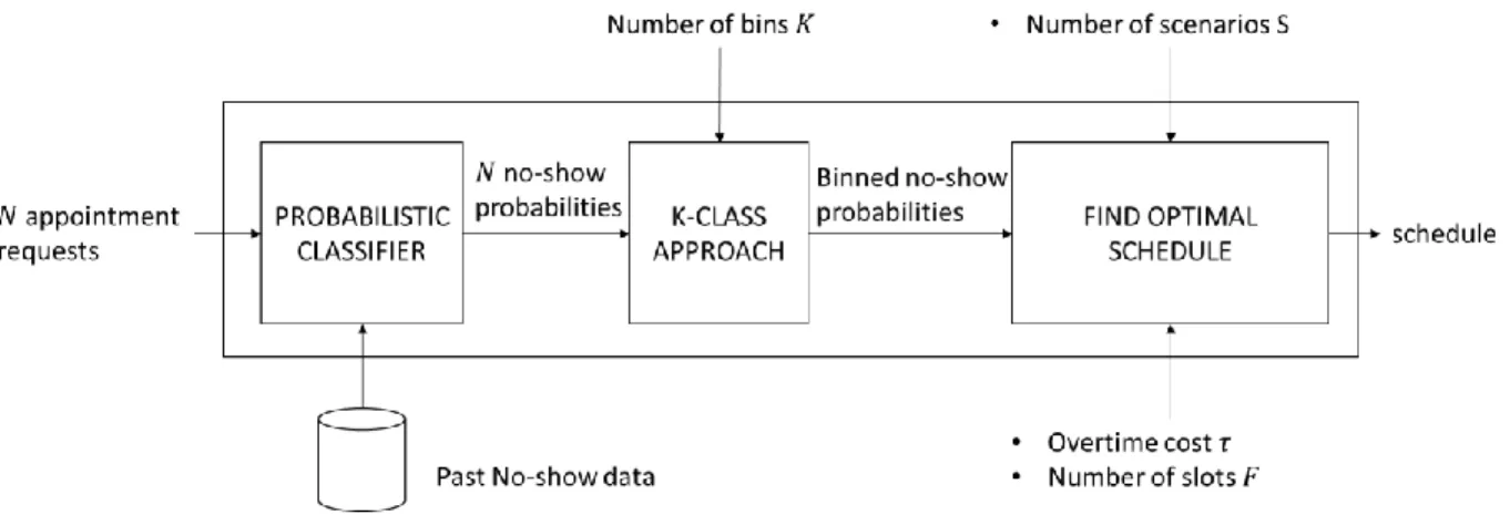
In this paper, we consider the appointment scheduling system depicted in Figure 2. The input is a set of 𝑁

appointment requests and the output is a schedule, that is, an assignment of each appointment request to an appointment slot of a clinic session.

Figure 2: Scheduling system developed in this study.

The first step consists of predicting the no-show probability of each appointment request. This task is performed by a probabilistic classifier previously trained with past no-show data. The next section illustrates the construction of a probabilistic classifier on real-world appointment data.

In the second step of our procedure, we may decide to partition the no-show probabilities into 𝑘 ≤ 𝑁 bins. After this 𝑘-class procedure, the no-show probabilities are modified so that all appointment requests in the

same class have the same no-show probability. The purpose of this step is to measure the performance of the existing methods, which utilizes values of 𝑘 of 1 or 2, and compare it to the performance of utilizing larger values of 𝑘 (i.e., 𝑘 = 3,4, … , 𝑁).

The third and last step of our procedure employs a stochastic mixed integer program to find the optimal schedule. The input of this problem is composed of the binned no-show probabilities, the number of slots and the ratio between overtime cost and waiting time cost, as well as other parameters that can be tuned to obtain a heuristic scheduling procedure. Next, we illustrate the details of these components one by one.

Step 1: Deriving No-Show Probabilities from a Probabilistic Classifier

In a real-world setting, the individual no-show probabilities are obtained from a prediction model trained with past no-show data. Predicting no-shows is a binary classification problem, where the positive class is composed of the appointment requests that no-show and the negative class is composed of the appointment requests that show. To solve this problem, a classifier must be trained on past no-show data and employed to predict the no-show outcome of future appointment requests. In our context, in order to obtain individual no-show probabilities, we need a so called probabilistic classifier, a classifier that is capable of providing not only a binary no-show outcome but also a probability of being a no-show.

Some classifiers are probabilistic by nature (e.g., logistic regression), in the sense that their raw output is already a probability of being a no-show. Others are capable of labeling each appointment request with a

numeric “no-show score” which, despite not being an actual probability, is related to the probability of no-show. As explained by Niculescu-Mizil and Caruana (2005), a common technique to translate these numeric scores into probabilities is the Platt’s method (Platt, 1999), which consists of building a logistic regression model that predicts the binary no-show outcome given the no-show score. To measure the

quality of the probabilities, we use the Brier’s score (Brier, 1950), a common metric used to evaluate the quality of calibrated probabilities based on the corresponding binary outcomes. The score computes the mean squared difference between the predicted probabilities and the real binary outcome; the lower the

Brier’s score, the higher the quality of the probabilities.

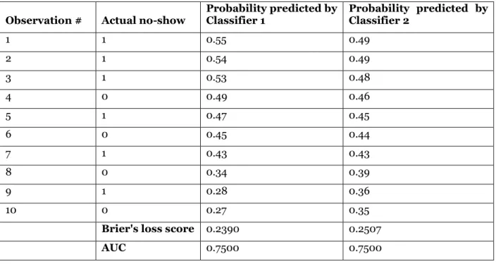
We prefer using the Brier’s score over more traditional prediction metrics typically used for binary classification, which measure the quality of the binary predictions (such as the accuracy or the F-score) or the quality of the ranking (such as the Area Under the Curve), and not that of the probabilities obtained. Table 1 shows a small example of the predictions made by two classifiers that achieve the same AUC but

Observation # Actual no-show Probability predicted by Classifier 1 Probability predicted by Classifier 2 1 1 0.55 0.49 2 1 0.54 0.49 3 1 0.53 0.48 4 0 0.49 0.46 5 1 0.47 0.45 6 0 0.45 0.44 7 1 0.43 0.43 8 0 0.34 0.39 9 1 0.28 0.36 10 0 0.27 0.35

Brier's loss score 0.2390 0.2507

AUC 0.7500 0.7500

Table 1. Example of two classifiers with the same AUC but different Brier’s score

The reason for the discrepancy between AUC and Brier’s score lies in the fact the probabilities predicted by

classifier 1 are closer to the actual class than the probabilities predicted by classifier 2, even if both classifiers rank the observations in order of no-show probability in the same way.

To achieve the best possible performance, several probabilistic classifiers should be calibrated on the available data using a cross-validation procedure or hold-out sample. The classifier obtaining the lowest cross-validated or out-of-sample Brier’s score should be finally chosen. The next subsection illustrates an in-depth case study where we follow a similar calibration process on three real-world data sets. We also provide a tool that practitioners can readily use to construct a probabilistic classifier using their data.

Case-study on real-world data

Here, we illustrate our procedure to build probabilistic classifiers on real-world data. The goal of this subsection is twofold:

(1) To serve as a step-by-step guide for practitioners interested in predicting no-shows at their clinic. To this end, we provide a Jupyter notebook that practitioners can readily use on their data set (at

https://github.com/samorani/appointment-scheduling-utilities/tree/master/select%20best%20classifier).

(2) To investigate the distribution of the individual no-show probabilities in real-world domains. This information is used in the next section to choose the parameters of our simulation study.

Our first data set is from fully anonymized, administrative records of 108,515 scheduled, in-person, weekday appointments from a local primary care clinic. The features include past no-show history, age, appointment lead time, day of the week, month of the year, and flags for whether or not the appointment was a follow-up or if the patient had multiple appointments scheduled in the same day. Of the 108,515 appointment requests, 11.69% resulted in a no-show. Because the no-show rate is approximately 12%, we call this data set VA-12.

Our second data set, which we call 30, is built by increasing the no-show rate of our first data set, VA-12, to 30%. This new no-show rate is obtained by removing from the original data set a random subset of the showing appointments. A no-show rate of 30% can be common in real-world clinics; with Daggy et al. (2010) reporting primary care clinic no-show rates between 14% and 50%.

For each of the two data sets, we built a probabilistic classifier as follows. The first step consists of partitioning the available data into a calibration set (80% of the data) and a test set (20% of the data). The calibration set is used to identify the best performing classification technique, whereas the test set is used to estimate its performance and to obtain the no-show probabilities that will be used throughout our experiments.

Considering only the calibration set, we considered the following classification techniques: Random Forest, Naïve Bayes, Logistic Regression, Decision Tree, AdaBoost, and Discriminant Analysis. For each classification technique, we performed the following steps:

1. We executed a 10-fold cross validation on the calibration set. At each iteration of the cross validation, the current classification technique is used to train a classifier with 90% of the calibration set, which is subsequently employed to label the remaining 10% with a predicted no-show score. To perform a fair comparison among the classification techniques, we employed the default parameters (provided by the scikit-learn package) for each classification technique. At this point, the current classification technique has labeled each observation in the calibration set with a no-show score.

2. We translated the no-show scores into probabilities using Platt’s method, in order to build a probabilistic classifier. That is, we built a logistic regression model on the calibration set, where the independent variable is the no-show score and the dependent variable is the actual 0-1 no-show outcome. That logistic regression model was then used to label each observation of the calibration set with a no-show probability. This second step was performed for every classification technique except logistic regression, as the output of logistic regression is a set of no-show probabilities.

3. We selected the classification technique that performed the best on the calibration set, as follows. we considered the no-show probabilities derived in the previous step to compute both the AUC and the Brier’s score obtained on the calibration set. The AUC measures how well the current classification technique ranks the observations from the most likely to no-show to the least likely to no-show, whereas

the Brier’s score measures how accurate the no-show probabilities are, on average.

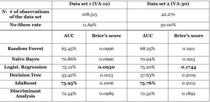
The cross-validated AUC and Brier’s score obtained by our classification techniques on the calibration set are reported in Table 2.

Data set 1 (VA-12) Data set 2 (VA-30)

N: # of observations

of the data set 108,515 42,270

No-Show rate 11.69% 30.00%

AUC Brier’s score AUC Brier’s score

Random Forest 65.45% 0.0996 68.25% 0.1911 Naïve Bayes 70.86% 0.0990 70.94% 0.1915 Logist. Regression 75.12% 0.0930 75.20% 0.1744 Decision Tree 53.42% 0.1013 57.63% 0.2019 AdaBoost 75.95% 0.1006 75.76% 0.2012 Discriminant Analysis 72.34% 0.0989 72.32% 0.1892

Table 2. Cross-validated AUC and Brier’s score obtained by several classification

techniques on the calibration set. Best classification technique according to either AUC or

Brier’s score are in bold.

Table 2 shows that for both of our data sets, AdaBoost was the technique that obtained the best (largest) AUC, whereas Logistic Regression was the technique that obtained the best (smallest) Brier’s score. To

that minimizes the Brier’s score, we analyzed the test set, limiting our analysis to AdaBoost and Logistic

Regression.

For each data set, we built one Logistic-Regression-based and one AdaBoost-based probabilistic classifier as follows. For Logistic Regression, we built a Logistic Regression model using the entire calibration set; this model can be readily used to predict no-show probabilities of test data. For AdaBoost, we built a probabilistic classifier by cascading the following two components. First, we trained an AdaBoost classifier on the entire calibration set and used it to obtain the no-show scores on the calibration set. Second, we built a logistic regression model that uses these no-show scores on the calibration set to predict the actual no-show outcomes of the calibration set. The no-show probability of a test appointment request can be obtained by first using the AdaBoost classifier to obtain a no-show score, and then employing the logistic regression model to translate the no-show score into a no-show probability.

Next, we analyzed the test set in order to achieve two objectives:

1. To check that our probabilistic classifier did not overfit the calibration set, and

2. To collect the no-show probabilities obtained on the test set, with the goal of using them in our second and third set of computational experiments.

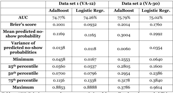
To achieve the first objective, we used our probabilistic classifiers to label each observation in the test set with its no-show probability. Then, we computed and recorded the AUC and Brier score obtained on the test set and compare them to the ones obtained during the cross validation procedure previously executed on the calibration set. For all probabilistic classifiers, the test-set AUC and Brier’s score are similar to those obtained in the calibration set, suggesting that our classification methods did not suffer from overfitting. To achieve the second objective, we simply recorded the no-show probabilities obtained by each probabilistic classifier. In our second and third set of computational experiments, we will repeatedly sample with replacement 𝑁 observations, use their no-show probabilities to schedule them optimally, and then finally use their real show outcome to evaluate the schedule. Summary statistics of the test-set no-show probabilities are reported in Table 3.

Data set 1 (VA-12)

Data set 2 (VA-30)

AdaBoost

Logistic Regr.

AdaBoost

Logistic Regr.

AUC

74.77%

74.26%

75.79%

75.02%

Brier’s score

0.1001

0.0932

0.2014

0.1760

Mean predicted

no-show probability

0.1169

0.1165

0.3004

0.2992

Variance of

predicted no-show

probabilities

0.0138

0.0118

0.0060

0.0354

Minimum

0.0458

0.0167

0.2553

0.0640

25

_percentile

_0.0560

_0.0537

_0.2805

_0.1600

50

_percentile

_0.0700

_0.0796

_0.2954

_0.2386

75

_percentile

_0.1156

_0.1338

_0.3178

_0.3840

Maximum

0.8853

0.8888

0.3786

0.9614

Table 3. AUC, Brier’s score, and summary statistics of the predicted no-show probabilities obtained by Logistic Regression and AdaBoost on the test set.

In summary, this section illustrated how we predicted no-show probabilities at the level of the individual appointment request. On our data sets, we identified two classification techniques, AdaBoost and Logistic

Step 2: The

𝒌

-class Approximation

Existing work in appointment scheduling assumes that all requests have the same no-show probability or that requests have either a low or a high no-show probability (Robinson & Chen 2010, LaGanga & Lawrence 2012, Zacharias & Pinedo 2014). In contrast, our main claim is that using more levels of no-show probabilities results in a better performance. To substantiate our claim, we introduce a procedure, called

𝑘-class approximation, which “bins” the individual no-show probabilities obtained by the classifier into 𝑘

classes.

In particular, given 𝑁 no-show probabilities, the 𝑘-class approximation modifies them so that they belong to 𝑘 classes of probabilities, with 𝑘 ranging from 1 to 𝑁. The probabilities are clustered into 𝑘 clusters using

𝑘-means (Kanungo et al. 2002), so that an appointment request’s new no-show probability is set to the average no-show probability of the cluster to which it belongs. Thus, the 1-class approximation sets each no-show probability to the 𝑁 requests’ average no-show probability, the 2-class approximation sets each no-show probability to either a “low” level or a “high” level, whereas the 𝑁-class approximation leaves the original no-show probabilities unchanged. We show that the 𝑁-class approximation results in better-quality schedules than the 1-class and the 2-class approximations.

To see the impact of the 𝑘-class approximation on the optimal schedule and to demonstrate that the 𝑁-class approximation is optimal, let us consider a small example with 𝑁 = 6 appointment requests that need to be scheduled in 𝐹 = 4 slots. Suppose that the no-show probabilities estimated by the classifier are:

[0.800 0.500 0.300 0.200 0.100 0.010]

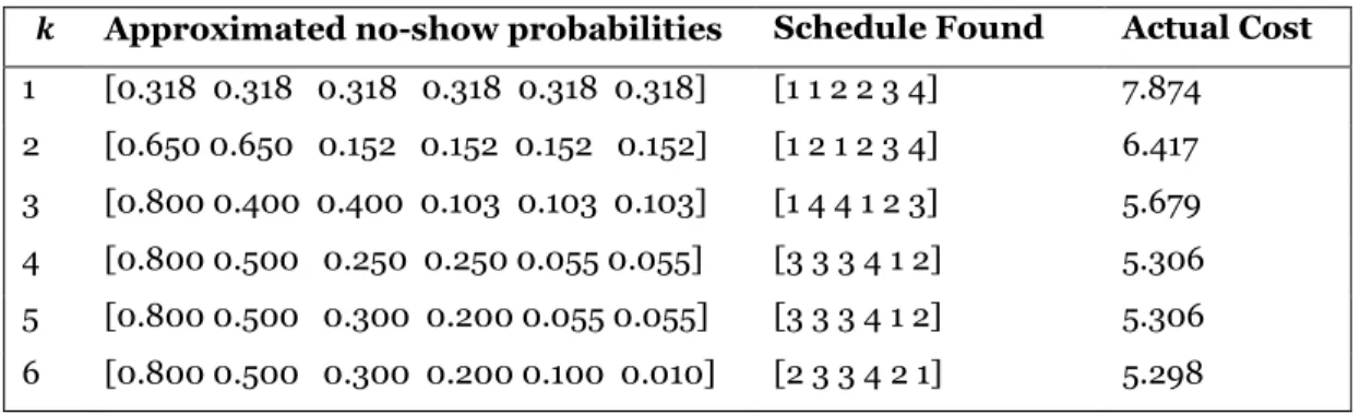
For each value of 𝑘= 1,…,6, Table 4 reports the approximated probabilities and the optimal schedule found using the approximated probabilities by the methodology illustrated in the next section.

The schedule is reported as vector whose 𝑖-th element is the slot number (from 1 to 4) where the 𝑖-th appointment request was scheduled. For example, the optimal schedule for 𝑘 = 6 consists of assigning the 6th _{patient (the one with the lowest no-show probability) to the first slot, then the 1}st _{and 5}th _{patients to the}

second slot, the 2nd _{and 3}rd _{patients to the third slot, and the 4}th _{patient to the fourth slot.}

𝒌 Approximated no-show probabilities Schedule Found Actual Cost 1 [0.318 0.318 0.318 0.318 0.318 0.318] [1 1 2 2 3 4] 7.874 2 [0.650 0.650 0.152 0.152 0.152 0.152] [1 2 1 2 3 4] 6.417 3 [0.800 0.400 0.400 0.103 0.103 0.103] [1 4 4 1 2 3] 5.679 4 [0.800 0.500 0.250 0.250 0.055 0.055] [3 3 3 4 1 2] 5.306 5 [0.800 0.500 0.300 0.200 0.055 0.055] [3 3 3 4 1 2] 5.306 6 [0.800 0.500 0.300 0.200 0.100 0.010] [2 3 3 4 2 1] 5.298

Table 4: Examples of schedules found using different 𝒌-class approximations

This example shows that the optimality condition found by Zacharias and Pinedo (2014) can be relaxed: they prove that patients with a 0% no-show probability should all be assigned to slots at the beginning of the schedule without any overbooking. However, many schedules in Table 4 show that the appointment requests scheduled at the beginning of the session without overbooking do not necessarily have a no-show probability exactly equal to 0%. For instance, for 𝑘 = 5 the fifth and sixth patients are assigned to the first two slots without any overbooking even if their no-show probability is 5.5%.

The actual cost is the expected cost of the schedule found, when evaluated using the original no-show probabilities. Note that when 𝑘 = 𝑁, the schedule found is the one with the lowest actual cost (i.e, it is the optimal schedule), because it is constructed using the original no-show probabilities. However, note the marginal improvement obtained by increasing 𝑘 by one decreases with 𝑘; this finding will be analyzed further in our computational experiments.

Step 3: Finding the Optimal Schedule

In this section, we illustrate our solution method for the scheduling problem with individual no-show probabilities. We consider an outpatient clinic where one provider sees patients sequentially. Appointments are scheduled in 𝐹 consecutive appointment slots of equal length. We assume that patients who show are punctual and that the time taken for each appointment is constant and equal to the length of each appointment slot.

The input of the problem is a set of 𝑁“appointment requests” (or, more simply, “requests”); the output is

an assignment of the appointment requests to appointment slots. Each request must be assigned to exactly one appointment slot, but each appointment slot may be assigned to more than one request (i.e., it may be overbooked). The 𝑖-th appointment request (𝑖 = 1, … , 𝑁) is labeled with the probability, 𝑞𝑖, that the patient will not show up for his or her appointment. We previously showed how to derive these no-show probabilities. Our methodology is defined for individual no-show probabilities (i.e., the 𝑁-class approach); however, as we discuss later in detail, the same methodology can be employed even if requests are clustered in classes of no-show probabilities (e.g., the 1-class approach or the 2-class approach).

The objective of the problem is to schedule appointment requests in order to minimize a weighted average

of the patients’ waiting time and the provider’s overtime. Waiting time cost is incurred whenever patients start their appointment late, at a rate of 𝜔 dollars for every time unit of delay incurred by any patient; overtime cost is incurred whenever the provider finishes seeing the patients after the nominal end time of the clinic session (i.e., after 𝐹 time units from the start), at a rate of 𝜏 dollars for every time unit of overtime. Without loss of generality, we fix the waiting time cost to 𝜔 = 1, and we vary the overtime cost 𝜏. Our notation is reported in Table 5.

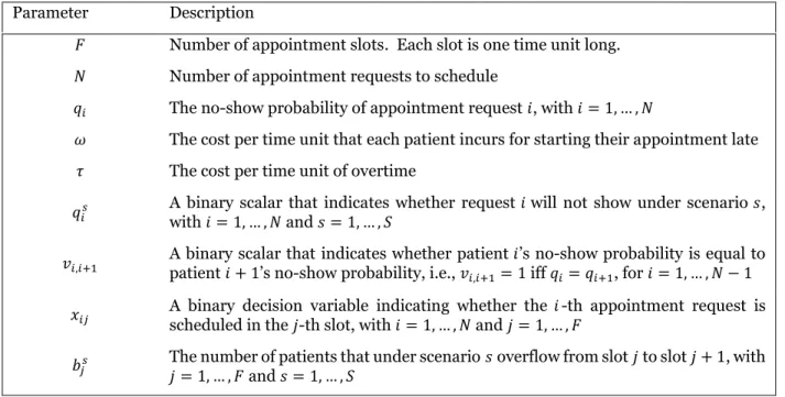
We model the scheduling problem as a stochastic mixed integer linear program. First, without loss of generality, we assume that the no-show probabilities 𝑞𝑖 provided as input are pre-sorted by increasing probability of no-show, that is, 𝑞𝑖≤ 𝑞𝑖+1 for 𝑖 = 1, … , 𝑁 − 1. We will later explain that this ordering will enable us to speed up the computation time.

Parameter Description

𝐹 Number of appointment slots. Each slot is one time unit long. 𝑁 Number of appointment requests to schedule

𝑞𝑖 The no-show probability of appointment request 𝑖, with 𝑖 = 1, … , 𝑁

𝜔 The cost per time unit that each patient incurs for starting their appointment late

𝜏 The cost per time unit of overtime

𝑞𝑖𝑠

A binary scalar that indicates whether request 𝑖 will not show under scenario 𝑠, with 𝑖 = 1, … , 𝑁 and 𝑠 = 1, … , 𝑆

𝑣𝑖,𝑖+1

A binary scalar that indicates whether patient 𝑖’s no-show probability is equal to patient 𝑖 + 1’s no-show probability, i.e., 𝑣𝑖,𝑖+1= 1 iff 𝑞𝑖= 𝑞𝑖+1, for 𝑖 = 1, … , 𝑁 − 1

𝑥𝑖𝑗 A binary decision variable indicating whether the _{scheduled in the 𝑗-th slot, with 𝑖 = 1, … , 𝑁 and 𝑗 = 1, … , 𝐹}𝑖-th appointment request is

𝑏𝑗𝑠 The number of patients that under scenario _{𝑗 = 1, … , 𝐹 and 𝑠 = 1, … , 𝑆} 𝑠 overflow from slot 𝑗 to slot 𝑗 + 1, with

Table 5. Notation

Second, given the no-show probabilities 𝑞1, 𝑞2, …, 𝑞𝑁, we build 𝑆“no-show” scenarios, each corresponding to one particular realization of no-shows: that is, each scenario corresponds to the subset of patients that will not show up. Since there are 2𝑁 _{subsets of 𝑁 requests, the total number of scenarios is 𝑆 = 2}𝑁_. Mathematically, each scenario 𝑠 (𝑠 = 1, … , 𝑆) is represented by a binary vector [𝑞1𝑠, 𝑞2𝑠, …, 𝑞𝑁𝑠] of length 𝑁,

whose components indicate which requests will result in a no-show under that scenario (𝑞𝑖𝑠 = 1 if request 𝑖 will not show under scenario 𝑠, and 0 otherwise). The probability 𝑝𝑠 _{of a scenario 𝑠 can be computed as the} joint probability to observe that all requests 𝑖 for which 𝑞𝑖𝑠= 1 will not show and that all requests 𝑖 such that 𝑞𝑖𝑠= 0 will show. That is:

𝑝𝑠= ∏ (𝑞𝑖𝑠𝑞𝑖+ (1 − 𝑞𝑖𝑠)(1 − 𝑞𝑖))

𝑖=1,…,𝑁 , 𝑠 = 1, … , 𝑆

Consider, for instance, a small problem with 𝑁 = 3 requests with no-show probabilities 𝑞1, 𝑞2, and 𝑞3. In this problem, there are 8 scenarios, each determining which subset of the three requests will not show up. For example, scenario [𝑞₁𝑠_{, 𝑞}

2𝑠, 𝑞3𝑠] = [0,0,1], which corresponds to the case where the first two patients show

up and the third one doesn’t, has a probability equal to (1 − 𝑞1)(1 − 𝑞2)𝑞3.

The cost incurred by the clinic, which varies from scenario to scenario, is computed by summing the costs incurred in each slot. In slot 𝑗 under scenario 𝑠, events unfold as follows:

1. The patients scheduled in slot 𝑗 who show up under scenario 𝑠 arrive at the beginning of slot 𝑗; 2. If there was a queue of patients waiting for the entire duration of the previous slot (slot 𝑗 − 1), these

patients “overflow” to slot 𝑗. The number of patients overflowing from slot 𝑗 − 1 to slot 𝑗 under scenario 𝑠 is determined by a decision variable 𝑏𝑗−1𝑠 .

3. The provider starts seeing one patient at the beginning of slot 𝑗 (as long as there is at least one patient in the system) and finishes seeing him/her at the end of slot 𝑗; if more than one patient are present in the system at the beginning of slot 𝑗, there will be one patient being served and 𝑏𝑗𝑠 patients waiting for the duration of the slot. Thus, in slot 𝑗 under scenario 𝑠 the clinic incurs a cost

equal to 𝜔 ∙ 𝑏𝑗𝑠 (i.e., a cost of 𝜔 for every patient waiting during slot 𝑗 under scenario 𝑠).

4. At the end of slot 𝑗, the patient being served exits the system. If other patients have been waiting during slot 𝑗 without being served, they overflow to the next slot.

5. At the end of the last slot, slot 𝐹, the provider continues seeing all remaining patients overtime at a rate of one patient per time unit. Thus, if there are 𝑏𝐹𝑠 patients at the end of the last slot under scenario 𝑠, the clinic will incur an overtime cost of 𝜏𝑏𝐹𝑠, as the provider will work overtime for 𝑏𝐹𝑠 time units, and a waiting time cost of 𝜔((𝑏𝐹𝑠− 1) + (𝑏𝐹𝑠− 2) + ⋯ + 1), as the number of patients waiting is 𝑏𝐹𝑠− 1 in the first overtime slot, 𝑏𝐹𝑠− 2 in the second overtime slot, etc. The last overtime slot to be considered is slot 𝐹𝑚𝑎𝑥_{, which we will show being equal to 𝑁.}

We now present a stochastic mixed integer linear programming model to find the optimal schedule for a given set of appointment requests. The assignment of requests to slots is determined by a set of binary decision variables, 𝑥𝑖𝑗, which are equal to 1 if request 𝑖 is scheduled to slot 𝑗 (for 𝑖= 1,…,𝑁 and 𝑗= 1,…,𝐹).

OPT-SCHED = 𝑚𝑖𝑛 ∑ 𝑝𝑠_{(𝜔 ∑ 𝑏} 𝑗𝑠 𝑗=1…𝐹𝑚𝑎𝑥 + 𝜏𝑏_𝐹𝑠) 𝑠=1…𝑆 Such that: ∑𝑗=1,…,𝐹𝑥𝑖𝑗 = 1 ∀𝑖 = 1 … 𝑁 (1) 𝑏_𝑗𝑠_{≥ 𝑏} 𝑗−1𝑠 + ∑𝑖=1…𝑁𝑥𝑖𝑗(1 − 𝑞𝑖𝑠)− 1 ∀𝑠 = 1 … 𝑆, 𝑗 = 1 … 𝐹𝑚𝑎𝑥 (2) ∑ 𝑥𝑖 𝑖𝑗 ≥ 1∀𝑗 = 1 … 𝐹 (3) 𝑥𝑖𝑗 ∈ {0,1}∀𝑠 = 1 … 𝑆, 𝑗 = 1 … 𝐹 𝑏𝑗𝑠≥ 0∀𝑠 = 1 … 𝑆, 𝑗 = 1 … 𝐹𝑚𝑎𝑥

The objective is to minimize the expected total cost of the schedule. Under each scenario, a given assignment of requests to slot (i.e., a schedule) will result in a scenario-dependent cost. Our model computes the expected cost of a schedule as the average cost obtained under each scenario 𝑠, weighted by

the probabilities 𝑝𝑠_{, 𝑠 = 1, … , 𝑆. Under each scenario, the cost is equal to the sum of the waiting time costs} and the overtime cost. Constraint set (1) states that each patient 𝑖 must be assigned to exactly one slot. Constraint set (2) sets the value of 𝑏𝑗𝑠, i.e., the number of patients overflowing from slot 𝑗 to slot 𝑗 + 1. It is at least equal to the number of patients overflowing into slot 𝑗, 𝑏𝑗−1𝑠 plus the number of arrivals in slot 𝑗 (∑𝑖=1…𝑁𝑥𝑖𝑗𝑞𝑖𝑠) minus one to account for the fact that one patient will be seen in slot 𝑗.

Constraint set (3) prevents the presence of empty slots in the schedule. As proved by LaGanga and Lawrence (2012), this is an optimality condition and we include it to reduce the solution space and, consequently, the computation time. Because of this condition, the maximum overtime suffered by the provider will be equal to 𝑁 − 𝐹 time units, which may be incurred by assigning one patient to each of the regular 𝐹 slots, and the remaining 𝑁 − 𝐹 patients to the last regular slot. If all patients in the last slot show

up, the provider will see the last patient in slot 𝑁 (i.e., 𝑁 − 𝐹 slots overtime). Thus, we set 𝐹𝑚𝑎𝑥 _{= 𝑁.}

Computational Results

In this section, we perform three sets of computational experiments to demonstrate the merit of our approach. In the first set of computational experiments, we show that using values of 𝑘 greater than those suggested by existing work (𝑘 = 1 or 2) results in significantly better-quality schedules. In the second set of experiments, we show that when our methodology is employed in a realistic setting (i.e., using the real-world data presented earlier), a small improvement in the Brier’s score may result in a large improvement

in schedule quality; furthermore, the quality of the schedules obtained is more closely related to the Brier’s

score than the AUC. In the third set of experiments, we extend our methodology to the case where appointment requests arrive sequentially (rather than being all available at the same time) and show that our findings keep being valid in that situation.

Computational Experiments 1: The Effect of Increasing

𝒌

In our first set of experiments, we study the impact of the approximation number 𝑘 on the performance of our solution method. In particular, we generated several instances of the scheduling problem, utilizing a different parameter combination for each instance.

For the experiments, the number of appointment requests is fixed to 𝑁 = 8. The reason for fixing the value of 𝑁 lies in the fact that each scheduling problem will be solved with all possible 𝑘-value approximations: 𝑘

= 1, 2, …, 𝑁. If more than one value of 𝑁 is used then some values of 𝑘 will be utilized only for certain values of 𝑁, making it harder to assess and interpret the effect of changing 𝑘. This number of appointments is common at outpatient clinics, where appointments are generally scheduled in two sessions per day (one in the morning with 𝑁 appointments and one in the afternoon with 𝑁 other appointments). To consider different no-show rates, we considered different values for the number of slots 𝐹 ∈ {5,6,7}. For each value of 𝐹, we fixed the mean no-show probability to 𝑞 = 1 − 𝐹/𝑁 (i.e., 37.5%, 25.0%, and 12.5%). The expression for 𝑞 results in an expected number of shows equal to the number of slots.

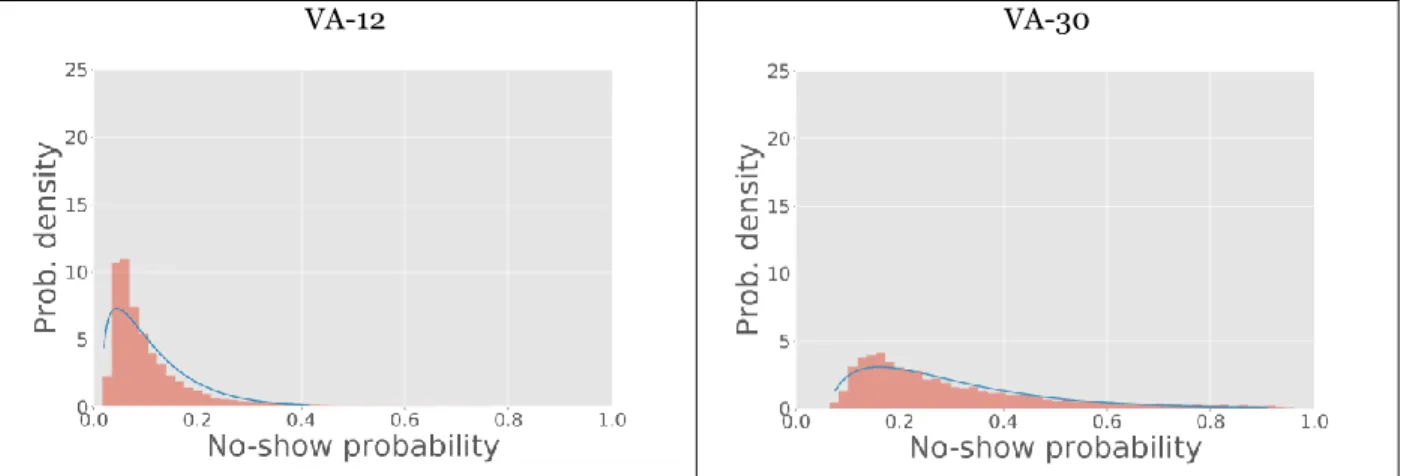
The 𝑁 no-show probabilities of the appointment requests were generated according to a 2-parameter 𝛽 -distribution with mean 𝑞 and variance 𝜎2_{∈ {0.005, 0.010, 0.020}. Our choice is justified by an analysis of} the no-show probabilities collected on our real-world data. In this analysis, we fit distributions to the data to find the best fit for the test-set no-show probabilities. We restricted our search to the distributions defined on the domain 0-1, so as to avoid generating infeasible probabilities: uniform, beta, triangular, and truncated normal. For both data sets, the best fit is obtained with the 𝛽-distribution. Figure 3 shows the distribution and fit of the 𝛽-distribution on the no-show probabilities obtained by Logistic Regression.

VA-12 VA-30

Figure 3. Fit of 𝜷-distribution on the test-set no-show probabilities obtained on our two data sets by Logistic Regression.

In the experiment, waiting time cost is fixed at 𝜔 = 1 per time unit; overtime cost is 𝜏 ∈{3,10}. For each of the 3 x 4 x 2 parameter combinations listed above, we generated 100 different scheduling problems by randomly sampling a set of 𝑁 no-show probabilities, for a total of 2,400 problem instances.

Each problem instance was solved through our mathematical model eight times, each time using a different

𝑘-value approximation (𝑘 = 1, … ,8). After solving each scheduling problem, we analytically computed and recorded the expected cost of the schedule obtained using the original no-show probabilities by averaging the cost incurred under each of the 2^N scenarios weighted by the probability of each scenario. Table 6 reports our results.

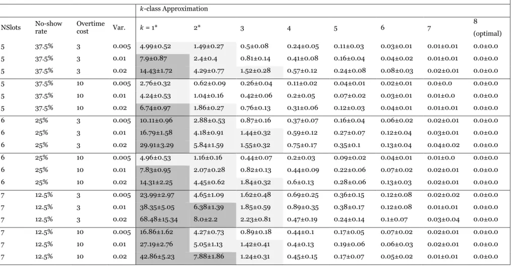
Each row in Table 6 is associated to a set of 100 randomly generated scheduling problems with the same number of slots, no-show probability distribution (mean and variance), and overtime cost. For each value of 𝑘, the table reports the average optimality gap and the 99% confidence interval obtained on the 100 schedules obtained.

The results suggest that the schedules obtained for larger values of 𝑘 are of higher-quality (i.e., with a smaller optimality gap) than the schedules obtained for smaller values of 𝑘. In particular, the optimality gap is largest for schedules obtained with 𝑘 = 1 and 𝑘 = 2, which are the values adopted in prior work. Interestingly, the average optimality gap is smaller than 1% under all parameter combinations when 𝑘 ≥ 4. We also found that while larger values of 𝑘 yield significantly better-quality schedules, the solution time increases dramatically with 𝑘. We will use this fact in our next set of experiments, where in order to solve larger scheduling problems in a shorter time, we consider values of 𝑘 smaller than 𝑁.

Computational Experiments 2: Validation on Real-World Data

In this subsection, we test our methodology on real-world data, by iteratively sampling appointment requests, predicting their individual no-show probability, and scheduling them.

First, as illustrated in section above where we discussed the real-world data case study, using the calibration set, we train an AdaBoost and a Logistic Regression classifier for each of our two data sets, 12 and VA-30. AdaBoost has the better (larger) AUC, whereas Logistic Regression has the better (smaller) Brier’s score. Here, we limit our analysis to these two classification techniques to show that a smaller Brier’s score (and not a larger AUC) results in a lower cost appointment schedule.

Table 6: Optimality gap % and its 99% confidence interval of the quality of 8-patient schedules obtained with the different K-class

approximations (k=1, 2,…,8) and different parameter combinations. Dark-grey cells indicate an optimality gap significantly larger than 5% (with 𝜶 = 0.01); light-grey cells indicate an optimality gap significantly larger than 1%.

*K = 1 and K = 2 are the approximations adopted in existing work.

𝑘-class Approximation

NSlots No-show _rate Overtime _cost Var. 𝑘 = 1* 2* 3 4 5 6 7 8

(optimal) 5 37.5% 3 0.005 4.99±0.52 1.49±0.27 0.5±0.08 0.24±0.05 0.11±0.03 0.03±0.01 0.01±0.01 0.0±0.0 5 37.5% 3 0.01 7.9±0.87 2.4±0.4 0.81±0.14 0.41±0.08 0.16±0.04 0.04±0.02 0.01±0.01 0.0±0.0 5 37.5% 3 0.02 14.43±1.72 4.29±0.77 1.52±0.28 0.57±0.12 0.24±0.08 0.08±0.03 0.02±0.01 0.0±0.0 5 37.5% 10 0.005 2.76±0.32 0.62±0.09 0.26±0.04 0.11±0.02 0.04±0.01 0.02±0.01 0.0±0.0 0.0±0.0 5 37.5% 10 0.01 4.24±0.53 1.04±0.16 0.42±0.06 0.2±0.05 0.07±0.02 0.03±0.01 0.01±0.0 0.0±0.0 5 37.5% 10 0.02 6.74±0.97 1.86±0.27 0.76±0.13 0.31±0.06 0.12±0.03 0.04±0.01 0.01±0.01 0.0±0.0 6 25% 3 0.005 10.11±0.96 2.88±0.53 0.87±0.16 0.37±0.07 0.16±0.04 0.06±0.02 0.02±0.01 0.0±0.0 6 25% 3 0.01 16.79±1.58 4.18±0.91 1.44±0.32 0.59±0.12 0.27±0.07 0.12±0.04 0.03±0.01 0.0±0.0 6 25% 3 0.02 29.91±3.29 5.84±1.59 1.55±0.32 0.75±0.17 0.35±0.1 0.13±0.04 0.04±0.02 0.0±0.0 6 25% 10 0.005 4.96±0.53 1.16±0.16 0.44±0.07 0.2±0.03 0.09±0.02 0.04±0.01 0.01±0.0 0.0±0.0 6 25% 10 0.01 7.83±0.95 2.07±0.28 0.82±0.13 0.44±0.09 0.22±0.06 0.07±0.02 0.02±0.01 0.0±0.0 6 25% 10 0.02 14.31±2.25 4.45±0.62 1.84±0.32 0.6±0.13 0.28±0.06 0.13±0.03 0.02±0.01 0.0±0.0 7 12.5% 3 0.005 23.99±2.97 4.65±1.09 1.62±0.48 0.69±0.25 0.36±0.15 0.12±0.08 0.02±0.02 0.0±0.0 7 12.5% 3 0.01 38.35±5.05 6.38±1.39 1.85±0.59 0.89±0.35 0.38±0.17 0.12±0.08 0.01±0.01 0.0±0.0 7 12.5% 3 0.02 68.48±15.34 8.0±2.2 2.23±0.81 0.47±0.19 0.24±0.14 0.1±0.07 0.03±0.04 0.0±0.0 7 12.5% 10 0.005 16.86±1.62 4.27±0.73 0.89±0.18 0.44±0.1 0.17±0.05 0.07±0.02 0.02±0.01 0.0±0.0 7 12.5% 10 0.01 27.19±2.76 5.05±1.13 1.42±0.41 0.4±0.13 0.19±0.06 0.06±0.03 0.02±0.01 0.0±0.0 7 12.5% 10 0.02 42.86±5.23 7.88±1.86 1.24±0.31 0.45±0.15 0.17±0.07 0.05±0.02 0.01±0.01 0.0±0.0

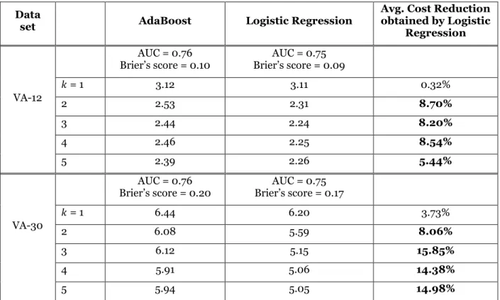
Second, we check which classifier leads to the better performance on the test set by computing the cost of the schedule obtained for each data set and for each classifier, as follows. For 500 iterations, we randomly sample with replacement 10 appointment requests from the test set and we employ the classifier to estimate their no-show probability. Then, we find the optimal schedule given the estimated no-show probabilities using different values of 𝑘, and finally we unveil the patients’ actual classes (no-show or show) and use it to evaluate the schedule. That is, the schedule is found from the no-show probabilities predicted by the

classifier, but its quality is evaluated using the patients’ real no-show outcomes from the test data. Table 7 reports the results.

Data

set AdaBoost Logistic Regression

Avg. Cost Reduction obtained by Logistic

Regression

VA-12

AUC = 0.76

Brier’s score = 0.10 Brier’s score = 0.09AUC = 0.75

𝑘 = 1 3.12 3.11 0.32% 2 2.53 2.31 8.70% 3 2.44 2.24 8.20% 4 2.46 2.25 8.54% 5 2.39 2.26 5.44% VA-30 AUC = 0.76

Brier’s score = 0.20 Brier’s score = 0.17AUC = 0.75

𝑘 = 1 6.44 6.20 3.73%

2 6.08 5.59 8.06%

3 6.12 5.15 15.85%

4 5.91 5.06 14.38%

5 5.94 5.05 14.98%

Table 7. Average schedule cost resulting in using no-show probabilities predicted by AdaBoost and Logistic Regression. Bold entries indicate that the cost reduction resulting

from Logistic Regression is significantly greater than zero at 𝜶 = 0.05.

We consider only values of 𝑘 up to 5 because larger values lead to only marginal improvement at the cost of much longer computational times. Also, to keep the average solution times below ten seconds, we only consider 500 scenarios (out of 2^10 = 1024 possible scenarios). Finally, to ensure a fair comparison between the two classification techniques, the appointment requests sampled in each of the 500 iterations are the same for each data set and for each classification technique.

For each data set (VA-12 and VA-30), Table 7 reports the AUC and Brier’s score obtained on the calibration

set. Additionally, for each value of 𝑘= 1,…,5, Table 7 reports the average cost obtained across the 500 iterations when building a schedule using the no-show probabilities estimated by Logistic Regression and AdaBoost. The last column reports the cost reduction percentage resulting when using Logistic Regression. Our results shows that logistic regression results in a lower scheduling cost than AdaBoost (bold entries indicate a significant difference) when 𝑘 ≥ 2. When 𝑘 = 1, the no-show probabilities estimated by the two methods are very similar, and consequently the schedules obtained do not have significantly different costs.

Because Logistic Regression has a lower Brier’s score and a lower AUC than AdaBoost, our results

corroborate our claim that when predicting no-show outcomes for appointment scheduling, the goal should be minimizing the Brier’s score rather than maximizing the AUC. Furthermore, our results suggest that by

improving the Brier’s score only marginally (by 0.01 on VA-12 and by 0.02 on VA-30) results in a very large cost reduction.

Finally, the table confirms the results of our first set of experiments: within the same classification technique, increasing 𝑘 results in a lower cost. In addition, the table suggests that the benefit of increasing

𝑘 is more evident when the classifier has a lower Brier’s score; this is because the lower the Brier’s score,

the more accurate the predicted probabilities, and the higher the benefit of not binning them.

Computational Experiments 3: Sequential Scheduling

So far, we have focused on the “static” scheduling problem, that is, we assumed that all 𝑁 appointment requests are available at the same time and can be scheduled all at once. In reality, however, appointment requests arrive sequentially (i.e., one at a time), and need to be scheduled without knowing the characteristics of future appointment requests (i.e., their number or their no-show probabilities).

As commonly done in other appointment scheduling work, we adapt the solution method we developed for the static scheduling problem to the sequential scheduling problem. The idea is to attempt to schedule the incoming appointment requests as closely as possible to one of the 500 optimal schedules found in the previous section. Since we do not know the future appointment requests, we do not know which of the 500 schedules to match. So, we follow all of them at the same time by measuring the deviation between each target schedule and the assignment of the patients already scheduled.

More precisely, for each data set (VA-12 and VA -30) and each classifier employed in the previous section (AdaBoost and Logistic Regression), we set up the solution method as follows. We create a set of available target schedules 𝑆 = {1,2, … ,500} that contain all of the 500 optimal schedules found in the previous section. Then, we characterize each target schedule 𝑠 = 1,2, … ,500 with two variables: first, the set of target assignments (𝑞_𝑖𝑠_{, 𝑗}

𝑖𝑠, 𝑎𝑖𝑠)𝑖=1,…,𝑁, where 𝑞𝑖 is patient 𝑖’s no-show probability, 𝑗𝑖 the slot assigned to 𝑖, and 𝑎𝑖𝑆 a Boolean variable indicating whether that assignment is still available (𝑎𝑖𝑆= 𝑇𝑟𝑢𝑒 at the beginning); second, the total deviation 𝑑𝑒𝑣𝑠 _{= 0, which will measure the deviation between the no-show probabilities of target} schedule 𝑠 and the no-show probabilities of the patients scheduled so far during the sequential scheduling. After setting up the variables of each target schedule, we generate a sequential scheduling problem by sequentially sampling 𝑁 = 10 appointment requests randomly from the test set. Then, we sequentially schedule each appointment request as follows. Let 𝑞 be the no-show probability of the current appointment request. We want to find the schedule 𝑠∗_{∈ 𝑆 that results in the smallest total deviation 𝑑𝑒𝑣}𝑠∗_{. To this end,} we identify the best-fitting available assignment for 𝑞 as 𝑖∗_{= 𝑎𝑟𝑔𝑚𝑖𝑛}

𝑠∈𝑆,𝑖:𝑎_𝑖𝑠=𝑇𝑟𝑢𝑒(𝑑𝑒𝑣𝑠+ |𝑞𝑖𝑠− 𝑞|); that is, if the current request was assigned to slot 𝑗𝑖𝑠 of schedule 𝑠, then the schedule’s total deviation 𝑑𝑒𝑣𝑠 would increase by |𝑞_𝑖𝑠_{− 𝑞|. After computing what would be the best assignment across all schedules, we select the} assignment that results in the smallest new total deviation. Let 𝑗∗ _{be the slot selected for the current} appointment request; we update the data structure of each schedule 𝑠 as follows: first, we identify an available assignment 𝑖 for slot 𝑗 (i.e., such that 𝑗𝑖𝑠= 𝑗 and 𝑎𝑖𝑠= 1); then, we set 𝑎𝑖𝑠= 0; finally, we update

𝑑𝑒𝑣𝑠_{= 𝑑𝑒𝑣}𝑠_{+ |𝑞}

𝑖𝑠− 𝑞|. If schedule 𝑠 has no available assignment 𝑖 for slot 𝑗, then 𝑠 cannot be anymore a target schedule, and we remove it from 𝑆. Table 8 reports the average cost obtained on 200 sequential scheduling problems by AdaBoost and Logistic Regression. As for Table 7, the AUC and Brier’s score

reported in Table 8 are relative to the calibration set.

Our results suggest that even in the case of sequential scheduling, the classifier that on the calibration set obtains the lower Brier’s score performs (on the test set) significantly better than the one with the larger AUC.

Data set AdaBoost Logistic Regression obtained by Logistic Cost Reduction Regression VA-12 AUC = 0.76 Brier’s score = 0.10 AUC = 0.75 Brier’s score = 0.09 2.60 2.38 8.46% VA-30 AUC = 0.76 Brier’s score = 0.20 AUC = 0.75 Brier’s score = 0.17 5.14 4.64 9.73%

Table 8. Average schedule cost resulting in using no-show probabilities predicted by AdaBoost and Logistic Regression in the sequential scheduling problem. Bold entries indicate that the cost reduction resulting from Logistic Regression is significantly greater

than zero at 𝜶 = 0.05.

Conclusion

Despite the existence of prior work that studies the causes of appointment no-shows, little effort has been spent to integrate the no-show predictions into an appointment scheduling system.

Existing work in appointment scheduling has either used a unique no-show probability for all appointment requests (i.e., the 1-class approach) or has considered two classes of patients (i.e., the 2-class approach). In contrast, this work considers any number of classes, up to the case where each appointment request has its own no-show probability (i.e., the 𝑁-class approach). To the best of our knowledge, ours is the only methodology that optimally schedules requests given their individual no-show probabilities. Our results show that considering more than 2 classes of no-show probabilities leads to higher-quality schedules. Some existing work that seeks to leverage no-show predictions to inform scheduling decisions has focused on finding the classification technique that maximizes the AUC (Goffman et al. 2017, Li et al. 2019). In contrast, our experiments on real-world data suggest that the classifiers with the largest AUC is not necessarily the one that leads to lower-cost schedules. In fact, we find that the Brier’s score is a more

suitable metric to use when selecting a classifier. We provide the code to guide practitioners to predict no-shows from their data.

Finally, our preliminary results show that a small improvement in the Brier’s score may result in a large reduction in scheduling cost. However, more research is needed to quantify the improvement caused by

reduction in Brier’s score.

There are several other opportunities for future research. First, our findings can be validated on other data

sets and classification techniques. Second, future studies can relax our assumptions of patients’ punctuality and constant service times. Third, it would be interesting to include the possibility for patients to express preferences on the appointment day and time, as in Feldman et al. (2014). Finally, we could deploy our system in an actual outpatient clinic and study how patients perceive the system. Because one of the

predictors is the patient’s past no-show behavior and because patients with high no-show probability tend to be scheduled in overbooked slots, it follows that our system tends to schedule likely no-shows into overbooked slots. This will result in longer waiting time, customer dissatisfaction, and -possibly- to the customer failing to show up again, which would further increase their no-show probability. Thus, an additional avenue for future research could be to empirically study if and how systems like ours affects patient no-show behavior.

In conclusion, our work shows that using probabilistic classifiers to predict no-shows can dramatically improve the quality of appointment schedules. More research is needed to develop guidelines on how to select a suitable classifier.

References

Brier, G.W., 1950. “Verification of forecasts expressed in terms of probability“. Monthey Weather Review, 78(1), pp.1-3.

Daggy, J., Lawley, M., Willis, D., Thayer, D., Suelzer, C., DeLaurentis, P.C., Turkcan, A., Chakraborty, S. and Sands, L., 2010. “Using no-show modeling to improve clinic performance”. Health Informatics Journal, 16(4), pp.246-259.

Feldman, J., Liu, N., Topaloglu, H. and Ziya, S., 2014. Appointment scheduling under patient preference and no-show behavior. Operations Research, 62(4), pp.794-811.

Gallucci, G., Swartz, W. and Hackerman, F., 2005. “Impact of the wait for an initial appointment on the rate of kept appointments at a mental health center”. Psychiatric Services, 56(3), pp.344-346.

Goffman, R.M., Harris, S.L., May, J.H., Milicevic, A.S., Monte, R.J., Myaskovsky, L., Rodriguez, K.L., Tjader, Y.C. and Vargas, D.L., 2017. “Modeling patient no-show history and predicting future outpatient appointment behavior in the veterans health administration”. Military medicine, 182(5-6), pp.e1708-e1714.

Harris, S.L., May, J.H. and Vargas, L.G., 2016. “Predictive analytics model for healthcare planning and scheduling”. European Journal of Operational Research, 253(1), pp.121-131.

Kanungo, T., Mount, D.M., Netanyahu, N.S., Piatko, C.D., Silverman, R. and Wu, A.Y., 2002. “An efficient k-means clustering algorithm: Analysis and implementation”. IEEE Transactions on Pattern Analysis & Machine Intelligence, (7), pp.881-892.

LaGanga, L.R. and Lawrence, S.R., 2007. “Clinic overbooking to improve patient access and increase

provider productivity”.Decision Sciences, 38(2), pp.251-276.

LaGanga, L.R. and Lawrence, S.R., 2012. “Appointment overbooking in health care clinics to improve

patient service and clinic performance”.Production and Operations Management, 21(5), pp.874-888. Li, Y., Tang, S.Y., Johnson, J. and Lubarsky, D.A., 2019. Individualized No‐show Predictions: Effect on Clinic Overbooking and Appointment Reminders. Production and Operations Management, 28(8), pp. 2068-2086.

Liu, N., Ziya, S. and Kulkarni, V.G., 2010. Dynamic scheduling of outpatient appointments under patient no-shows and cancellations. Manufacturing & Service Operations Management, 12(2), pp.347-364. Niculescu-Mizil, A. and Caruana, R., 2005, “Predicting good probabilities with supervised learning”.

In Proceedings of the 22nd international conference on Machine learning (pp. 625-632). ACM. Orlikowski, W.J. and Iacono, C.S., 2001. Research commentary: Desperately seeking the “IT” in IT

research—A call to theorizing the IT artifact. Information systems research, 12(2), pp.121-134.

Partin, M.R., Gravely, A., Gellad, Z.F., Nugent, S., Burgess Jr, J.F., Shaukat, A. and Nelson, D.B., 2016.

“Factors associated with missed and cancelled colonoscopy appointments at Veterans Health Administration facilities”. Clinical Gastroenterology and Hepatology, 14(2), pp.259-267.

Platt, J., 1999. “Probabilistic outputs for support vector machines and comparisons to regularized likelihood methods”. Advances in large margin classifiers, 10(3), pp.61-74.

Robinson, L.W. and Chen, R.R., 2010. “A comparison of traditional and open-access policies for appointment scheduling”. Manufacturing & Service Operations Management, 12(2), pp.330-346.

Samorani, M., LaGanga, L., 2015. “Outpatient appointment scheduling given individual day-dependent no-show predictions”. European Journal of Operational Research, 240(1), pp.245-257.

Srinivas, S. and Ravindran, A.R., 2018. “Optimizing outpatient appointment system using machine learning algorithms and scheduling rules: A prescriptive analytics framework”. Expert Systems with Applications, 102, pp.245-261.

U.S. Department of Veterans Affairs, Office of Inspector General. Audit of Veterans Health Administration’s efforts to reduce unused outpatient appointments, 2008. Available at

http://www.va.gov/oig/52/reports/2009/VAOIG-08-00879-36.pdf; accessed September 4, 2019. Whittle, J., Schectman, G., Lu, N., Baar, B. and Mayo-Smith, M.F., 2008. “Relationship of scheduling

interval to missed and cancelled clinic appointments”. The Journal of ambulatory care management, 31(4), pp.290-302.

Zacharias, C. and Pinedo, M., 2014. “Appointment scheduling with no‐shows and overbooking”. Production and Operations Management, 23(5), pp.788-801.