econ
stor
www.econstor.eu
Der Open-Access-Publikationsserver der ZBW – Leibniz-Informationszentrum Wirtschaft
The Open Access Publication Server of the ZBW – Leibniz Information Centre for Economics
Nutzungsbedingungen:
Die ZBW räumt Ihnen als Nutzerin/Nutzer das unentgeltliche, räumlich unbeschränkte und zeitlich auf die Dauer des Schutzrechts beschränkte einfache Recht ein, das ausgewählte Werk im Rahmen der unter
→ http://www.econstor.eu/dspace/Nutzungsbedingungen nachzulesenden vollständigen Nutzungsbedingungen zu vervielfältigen, mit denen die Nutzerin/der Nutzer sich durch die erste Nutzung einverstanden erklärt.
Terms of use:
The ZBW grants you, the user, the non-exclusive right to use the selected work free of charge, territorially unrestricted and within the time limit of the term of the property rights according to the terms specified at
→ http://www.econstor.eu/dspace/Nutzungsbedingungen By the first use of the selected work the user agrees and declares to comply with these terms of use.
Packham, Natalie; Schlögl, Lutz; Schmidt, Wolfgang M.
Working Paper
Credit gap risk in a first passage time
model with jumps
CPQF Working Paper Series, No. 22
Provided in cooperation with:
Frankfurt School of Finance and Management
Suggested citation: Packham, Natalie; Schlögl, Lutz; Schmidt, Wolfgang M. (2009) : Credit gap risk in a first passage time model with jumps, CPQF Working Paper Series, No. 22, http:// hdl.handle.net/10419/40179
C
CeennttrreeffoorrPPrraaccttiiccaallQQuuaannttiittaattiivveeFFiinnaannccee
CPQF Working Paper Series No. 22
Credit gap risk in a first passage time model with jumps Natalie Packham, Lutz Schlögl and Wolfgang M. Schmidt
Authors: Natalie Packham Lutz Schlögl
Assistant Professor for Quantitative Finance Fixed Income Quantitative Research Frankfurt School of Finance & Management Nomura International Plc
Frankfurt/Main London, UK
[email protected] [email protected] Wolfgang M. Schmidt
Professor of Quantitative Finance
Frankfurt School of Finance & Management Frankfurt/Main
November 2009
Publisher: Frankfurt School of Finance & Management
Phone: +49 (0) 69 154 008-0 Fax: +49 (0) 69 154 008-728 Sonnemannstr. 9-11 D-60314 Frankfurt/M. Germany
Credit gap risk in a first passage time model with jumps
Natalie Packham∗, Lutz Schl¨ogl†and Wolfgang M. Schmidt‡ November 2009
Abstract
The payoff of many credit derivatives depends on the level of credit spreads. In particular, credit derivatives with a leverage component are subject to gap risk, a risk associated with the occurrence of jumps in the underlying credit default swaps. In the framework of first passage time models, we consider a model that addresses these issues. The principal idea is to model a credit quality process as an Itˆo integral with respect to a Brownian motion with a stochastic volatility. Using a representation of the credit quality process as a time-changed Brownian motion, one can derive formulas for conditional default probabilities and credit spreads. An example for a volatility process is the square root of a L´evy-driven Ornstein-Uhlenbeck process. The model can be implemented efficiently using a technique called Panjer recursion. Calibration to a wide range of dynamics is supported. We illustrate the effectiveness of the model by valuing a leveraged credit-linked note.
Keywords: gap risk, credit spreads, credit dynamics, first passage time models, stochastic volatility, general Ornstein-Uhlenbeck processes
JEL classification: G12, G13, G24, C69
1
Introduction
Other than being subject exclusively to default risk, the payoff of some credit derivatives is determined explicitly by the level of CDS spreads, the spreads of credit default swaps. In this case, the dynamics of CDS spreads play a significant role in product valuation. Examples of such products are default swaptions and credit derivatives with a leverage component. The latter are in addition sensitive to gap risk, a risk that is linked to the occurrence of jumps in the evolution of credit spreads, even if such jumps do not lead to
default. An example of such a product, the leveraged credit-linked note, is described in
detail in Section 2.4.
There is a significant amount of empirical research that indicates that credit spreads are subject to sudden and unexpected jumps [Johannes, 2000], [Zhou, 2001], [Das, 2002], [Dai and Singleton, 2003], [Tauchen and Zhou, 2006] and [Zhang et al., 2008]. In a recent empirical study on credit spreads, [Schneider et al., 2007] observe that CDS spreads ex-hibit frequent positive jumps, which typically affect CDS spreads of all maturities. These jumps are attributed to the arrival of bad news. Good news also affect the whole maturity spectrum, but tend to propagate gradually.
The model considered here, a first passage time model with jumps, captures these stylised facts and is suitable for valuing credit derivatives that are subject to gap risk.
∗
Natalie Packham, Centre for Practical Quantitative Finance, Frankfurt School of Finance & Manage-ment, Sonnemannstr. 9-11, 60314 Frankfurt am Main. [email protected]
†
Lutz Schl¨ogl, Fixed Income Quantitative Research, Nomura International Plc, [email protected]
‡
Wolfgang M. Schmidt, Centre for Practical Quantitative Finance, Frankfurt School of Finance & Man-agement, Sonnemannstr. 9-11, 60314 Frankfurt am Main. [email protected]
There are generally two approaches to modelling credit risk: the structural and the reduced-form approach. In reduced-form models, default is not linked to economic vari-ables, but is an unpredictable Poisson-type event, and the main object of the modeller’s attention is the hazard rate of the jump process describing default. This approach has been overwhelmingly popular with practitioners, its main advantage is its tractability: It is generally straightforward to fit a given term structure of CDS spreads and the techniques are very similar to those of interest rate modelling. The literature on this type of models is vast, the papers by [Jarrow and Turnbull, 1995], [Lando, 1998] and [Duffie and Singleton, 1999] are only a few classic examples.
From the point of view of spread dynamics, modelling the default time as a totally unpredictable stopping time is not entirely satisfactory. Even with a low initial hazard rate, such a model will assign a non-negligible probability to the possibility of the credit defaulting without a prior movement in the credit spread. Defaults of this type are very uncommon in practice. The default swap market is efficient enough that default events are almost always preceded by a significant widening of credit spreads. It is this spread widening that is the real jump event that a market participant needs to worry about.
The ability of a model to assign probability mass to spread widening scenarios is con-strained by the probability assigned to defaults in low spread scenarios, as the model must fit the initial credit spread. From a practical point of view, failure to assign enough prob-ability to spread widening scenarios can lead to a dangerous underpricing of credit spread gap risk. The phenomenology of default that we are trying to capture is the following: a credit with a low default swap spread does not default “out of the blue”, but rather some kind of regime change takes place, causing the credit spread to widen, after which the credit may either default or eventually recover.
We implement this idea via a first passage time model where a credit quality process
exhibits stochastic volatility. In fact, the volatility process is a Levy-driven Ornstein-Uhlenbeck process. A jump in the volatility process is the “regime switch” we alluded to earlier. The current trend is to interpret the class of structural models in a wide sense to include any model where default is modelled as the first hitting time of a certain threshold by an abstract observable credit quality process. In this sense our model is structural, though the term “first passage time model” is technically more accurate. The structural approach, pioneered by [Merton, 1974], has been developed by [Black and Cox, 1976], [Longstaff and Schwartz, 1995], and many others.
As the name suggests, in a first passage time model, the computation of default proba-bilities is equivalent to computing the distributions of first passage times. The simplest case is that of a Brownian motion hitting a constant barrier, where a simple closed-form solution exists. This simple set-up however does not allow one to fit a given term structure of credit spreads. Furthermore, in reality, credit spreads exhibit strong jump dynamics. Several ex-tensions where the credit quality process is modelled by a jump-diffusion or a L´evy process were brought forward to overcome these problems, e.g. [Zhou, 2001], [Kiesel and Scherer, 2007], [Baxter, 2007] and [Cariboni and Schoutens, 2007]. However, in all of these cases, computing first passage times is intractable or computationally very demanding.
[Overbeck and Schmidt, 2005] propose a simple solution to the problem of calibrating a first passage time model to a term structure of credit spreads.by considering the first hitting time of a time-changed Brownian motion to a constant barrier. The time change is continuous, strictly increasing and deterministic. Because both the time change and the underlying Brownian motion are continuous, one can easily adapt the analytic formula from the simple Brownian case and obtain an analytic calibration to a term structure of default probabilities.
Our model builds directly on [Overbeck and Schmidt, 2005]. We consider a credit quality
increasing time change independent of the Brownian motion. The credit quality processX
can also be represented as an Itˆo integralX =R.
0σudWu with a Brownian motion W and a
volatility processσ. Our standard example for the volatility processσ is the square root of an Ornstein-Uhlenbeck process driven by a compound Poisson process. In the time-changed
Brownian motion interpretation, we can write X as Xt =BΛt with B a Brownian motion
and Λt =
Rt 0σ
2
udu. Because the time change Λ is continuous and independent of B, we
retain all the tractability of the deterministic case, while jumps in the volatilityσ induce jumps in the credit spreads, even though the credit quality processX is continuous.
The model and its properties are studied in detail in [Packham et al., 2009]. In the present paper, we focus on the implementation, calibration and on valuation of gap risk. Given the state of the credit quality process and its volatility, one can efficiently compute the whole term structure of default probabilities or credit spreads using a technique called Panjer recursion [Panjer, 1981]. Implementation then boils down to a combination of Monte Carlo simulation for determining the state of the credit quality process and numerical computation of term structures. Calibration to a given term structures is achieved by minimising the root mean square error of model and market term structures. We show that under suitable choices for the dynamics parameters the error of calibration to a term structure of CDS spreads is as small as 10−6 basis points, while at the same time the model may be calibrated to a wide range of dynamical behaviours. In particular, even though the CDS spread in the first passage time model vanishes as maturity of the underlying CDS is approached, thereby excluding short-term default events, one may approximate short-term default events by including the possibility of large jumps in the volatility.
The paper is structured as follows: in Section 2 we introduce some notation that is used throughout, and we treat in detail the valuation of CDS spreads and of leveraged credit-linked notes. In Section 3, we briefly introduce the Overbeck-Schmidt model and
the extended first passage time model with jumps. We state formulas for conditional
default probabilities, from which credit spreads may be determined, and we establish that jumps in the stochastic volatility of the credit quality process translate into jumps in CDS spreads. In Section 4, we derive the algorithm for efficiently computing term structures of default probabilities and credit spreads, given the state of the credit quality process and its volatility. Calibration to implied term structures is treated in Section 5. Since there are currently no liquid market instruments to calibrate the dynamics, we demonstrate the range of viable dynamics that may be obtained in the model; this is done in Section 6. We also discuss the individual parameters that govern the dynamics of the model. Finally, in Section 7, we apply the model to the valuation of leveraged credit-linked notes and default swaptions.
2
Credit derivatives
2.1 Notation
Throughout, let (Ω,F,(Ft)t≥0,P) be a complete probability space endowed with a filtration
(Ft)t≥0, representing the information available in the market. In particular,F0 isP-trivial.
We assume that (Ft)t≥0 satisfies the usual hypotheses, i.e., F0 contains all P-null sets
of F and (Ft)t≥0 is right-continuous. We also assume that the probability space is rich
enough to support any objects that we define. If not otherwise stated, all processes are (Ft)t≥0-adapted.
We assume thatPis a risk-neutral measure (presupposing existence of such a measure), that is,Pis a probability measure equivalent to the real-world probability measure and such that discounted prices areP-martingales. It follows that the market is free of arbitrage.
2.2 Credit default swaps
The fundamental product of the credit derivatives market is thecredit default swap (CDS). Given an underlying entity, such as a company, it is a contract between two counterparties, the protection buyer and the protection seller, that insures the protection buyer against the loss incurred by default of the underlying entity within a fixed time interval. The
protection buyer regularly pays a constant premium, the credit spread or CDS spread,
which is fixed at inception, up until maturity of the CDS or the default event, whichever occurs first. This stream of payments is termed thepremium leg of the CDS. In return, the protection seller agrees to compensate the protection buyer for the loss incurred by default of the underlying entity at the time of default in case this occurs before maturity. This
constitutes the protection leg of the CDS. The CDS spread that makes the value of the
premium leg and the protection leg equal is thefair CDS spread.
More precisely, letr ∈R+ denote the default-free interest rate, assumed to be constant
for simplicity. Furthermore, assume that the payment at default is a fraction (1−R) of
the notational amount, R ∈[0,1). Denote by τ the random time of the default event. In
our setup,τ is an (Ft)t≥0-stopping time. The distribution function of τ conditional on the
information flow (Ft)t≥0 is denoted by P(t, T) :=P(τ ≤T|Ft). Denote bys(t, T) the fair
credit spread at timet of a CDS with maturityT. Entering into a CDS involves no initial cash-flow, that is, the market value of a CDS at inception is 0; in other words, the discounted fair values of the premium and the default legs are equal. From these considerations, one can show that, on {τ > t}, the fair credit spread or fair CDS spread s(t, T) at time t is given by s(t, T) 1−R = RT t e −r(u−t)dP(t, u) RT t e−r(u−t)(1−P(t, u)) du . (1)
On{τ ≤t}or fort≥T, we sets(t, T) = 0. The mappingT 7→s(t, T) is theterm structure of credit spreads at time t. Given a term structure of CDS spreads s(t, T), T ≥ t, one can infer the risk-neutral default probabilities P(t, T), T ≥t, from Equation (1), and vice versa.
Themark-to-market valueof an existing CDS position is expressed as the cost of unwind-ing the transaction by enterunwind-ing into an offsettunwind-ing CDS position. Assume a CDS contract
with maturity T entered at time v ≤t from the point of view of the protection seller. On
{τ > t}, the value of the position at time tis
Vt=s(v, T) Z T t e−r(u−t)(1−P(t, u)) du−(1−R) Z T t e−r(u−t)P(t,du) = (s(v, T)−s(t, T)) Z T t e−r(u−t)(1−P(t, u)) du. (2) If default occurs prior toT, that is,τ < T, we setVτ =−(1−R).
2.3 Shape and dynamics of the term structure
The term structure of credit spreads has been extensively studied.1 Let us outline some
stylised facts about the shape and dynamics of the term structure. A wide variety of term structure shapes has been observed in the market, such as upward sloping, flat, hump-shaped and downward sloping curve, see for example [Helwege and Turner, 1999], [Zhou, 2001], [Fons, 1994] and [Helwege and Turner, 1999].
1The term credit spread also refers to theyield spread, which is the yield difference of defaultable and
default-free zero-coupon bonds of the same maturity. There are some subtle differences between yield spreads and CDS spreads, mainly due to factors such as liquidity of the underlying and restrictions regarding short-selling. However, we assume that stylised facts of the yield spread term structure that can be related to the credit risk component of the underlying entity apply to the CDS term structure as well.
Another common observation is that short-term credit spreads do not tend to zero as maturity tends to zero, but are significantly greater than zero, see e.g. [Duffie and Lando, 2001], [Zhou, 2001], [Duffie and Singleton, 2003, Ch. 3] and [Lando, 2004, Ch. 2]. This indicates that, for any time to maturity, market participants presume a positive probability of unexpected and instantaneous default.
There is also a significant amount of research that indicates that credit spreads are subject to jumps, i.e., in addition to continuous behaviour of credit spreads through time, credit spreads may change by sudden and unexpected jumps, see [Johannes, 2000], [Zhou, 2001], [Das, 2002], [Dai and Singleton, 2003], [Tauchen and Zhou, 2006], [Zhang et al., 2008]. [Schneider et al., 2007] infer the following empirical stylised facts for CDS spreads:
• A jump affects broad ranges of the CDS maturity spectrum. This is economically
motivated by the fact that unfavourable events usually affect contracts of both short and long maturities, and similarly, when expectations about the overall credit quality change, the entire term structure of CDS spreads reacts.
• Jumps in CDS spreads are mostly positive. The arrival of bad news such as financial
distress causes sudden upward moves in CDS spreads, because protection sellers de-mand higher compensation for bearing higher risk. Good news, on the other hand, tend to propagate gradually.
• The one-year CDS spread exhibits time-series variation different from CDS spreads
of higher maturities.
2.4 Leveraged credit-linked note
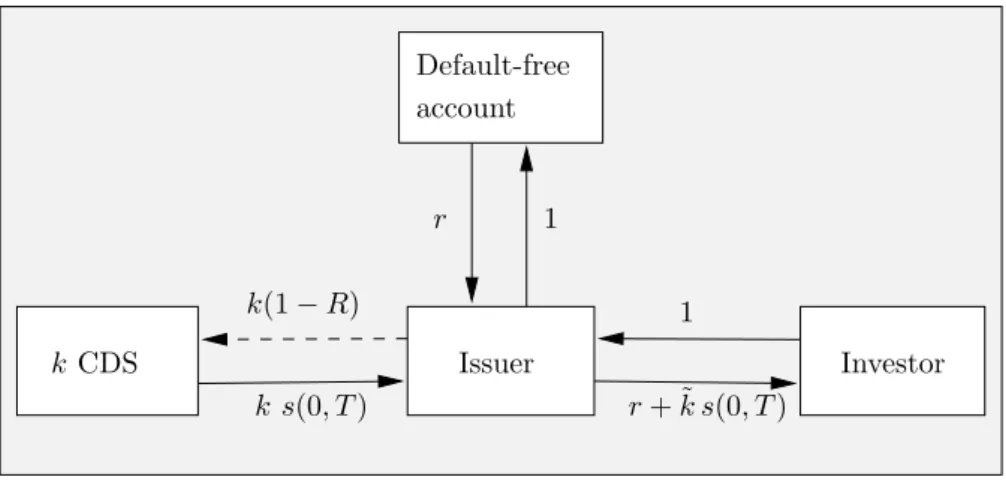
Let us now consider a credit derivative whose payoff is sensitive to the occurrence of jumps in credit spreads. A leveraged credit-linked note is particularly sensitive to jumps in CDS spreads, even if a jump does not lead to default.2 The principal idea is that an investor sells protection on an amount of default risk that is a multiple k, the leverage factor, of his investment amount. The motivation for taking leveraged exposure is to earn a certain multiple ˜k of the credit spread. Most likely, his investment will not suffice to compensate the loss incurred by default. Therefore, a trigger is agreed to terminate the structure while the cost of closing the position is still likely to be sufficiently covered by the investment amount. The cost of closing the position depends on the level of credit spreads, hence the investor is exposed mainly to spread risk and to default risk only to a lesser extent.
In more detail, the issuer structures the note as follows (see Figure 1): For simplicity, assume an investment amount of 1, which is deposited in a default-free account earning the risk-free rater. In addition, protection is sold by entering a fair CDS with notional k
earning a spread ofk s(0, T). The investor receives a fixed coupon until either maturity of the note or until a trigger event takes place. The size of the coupon is r+ ˜k s(0, T) with ˜
k s(0, T), ˜k ≤ k, the premium associated with the note, which is generated by the CDS position. The trigger event is defined as follows: denote by Vtk the mark-to-market value
at time t of the underlying CDS position with notional k. The trigger event takes place
at time S = inf{t ∈ (0, T] : Vtk ≤ −K}, with 0 < K ≤ 1 a pre-defined trigger level. At
S, the note is unwound by withdrawing the investment amount 1 from the deposit account
and by closing the CDS position, i.e., by entering the offsetting position, at a cost of−VSk. Observe that possibly VSk < −1, in which case the issuer must cover the missing amount required to unwind the CDS position. For this type of risk, called gap risk, the issuer is compensated with a premium of (k−k˜)s(0, T). In the case where VSk ≥ −1, the investor
2Acredit-linked note (CLN)is a note or bond paying an enhanced coupon to an investor for bearing the
Investor r+ ˜k s(0, T) 1 Issuer k s(0, T) k(1−R) kCDS account Default-free r 1
Figure 1: Leveraged credit-linked note with leverage factorkand notional 1. Cash flows at inception and while the note is alive.
receives the remainder of the structure, 1 +VSk. GivenK, valuation of the note essentially means determining the fair factor ˜k.
Clearly, the trigger time S depends on the evolution of the underlying CDS spread,
cf. Equation (2). Furthermore, the amount of the redemption payment max(1 +VSk,0) is
undetermined untilS. Assuming a model in which CDS spreads evolve continuously, the
mark-to-market value Vk evolves continuously as well. Unless a default takes place, the
trigger time is S = inf{t ∈ (0, T] : Vtk = −K} and VSk ≥ −1. Hence, a gap event takes place only when default happens without a prior trigger event. On the contrary, assuming a model in which CDS spreads are subject to jumps, upward jumps in CDS spreads translate into downward jumps in the mark-to-market value of the CDS, and possibly VSk <−1, so the issuer faces gap risk even when no default takes place.
In some models, we can determine the fair factor ˜kby no-arbitrage arguments. Assume
first that CDS spreads evolve continuously through time, so Vk evolves continuously as
well. Moreover, assume that there is no risk of an unpredictable jump-to-default (i.e., there is no default “totally out of the blue”). In this case, the trigger time isS= inf{t∈(0, T] :
Vtk =−K} and there is no gap risk at all, and the fair factor is ˜k=k. Now suppose that CDS spreads are constant, so the note is exposed to default risk only (in which caseVtk= 0, sinces(t, T) =s(0, T), for all t∈[0, T)). The trigger time then coincides with the default time, in which case the investor loses his invested capital. The payoff of this position is equivalent to the payoff of a short position in 1/(1−R) CDS, so ˜k= 1/(1−R).
Regardless of any model assumption, we can infer upper and lower bounds for the factor ˜
k. The upper bound is k as the note’s spread pickup is funded by the underlying CDS
position. To determine the lower bound, observe that the investor in the leveraged note is exposed to default risk and additionally to spread risk. An investor in a CDS position with notional 1/(1−R) is exposed to the same loss in case of default, but may terminate the investment at the same trigger timeS with a smaller loss. Hence, ˜k >1/(1−R).
To determine the factor ˜k, consider the cash flows to the note issuer discounted to time 0. Observe that the cash flows to the issuer isolate the gap risk component. The risk-neutral
value of these cash flows is given by V0gap=E (k−˜k)s(0, T) Z T 0 e−ru1{S>u}du−e−rS max(−VSk−1,0) = (k−˜k)s(0, T) Z T 0 e−ruP(S > u) du − Z (0,T]×(1,∞) e−ru(x−1)P(S ∈du,−VSk∈dx). (3)
The fair gap risk fee is obtained by setting V0gap= 0, i.e.,
(k−˜k)s(0, T) = R (0,T]×(1,∞)e −ru(x−1)P(S ∈du,−Vk S ∈dx) RT 0 e−ruP(S > u) du . (4)
The gap risk component in the valuation formula (3) is an option with payoff max(−VSk−
1,0) at time S, which the note issuer sells to the investor. The option premium is the
stream of payments RT
0 (k−˜k)s(0, T)1{S>u}du that is earned while the note is alive, so
that Equation (3) may be interpreted as the valuation formula for a gap option.
Clearly, to value a gap option requires a model that includes jumps in the evolution of credit spreads.
3
First passage time model with jumps
In this section we introduce a first passage time model that includes jumps in the evolution of credit spreads. The model is an extension of the Overbeck-Schmidt model, which we introduce first. The proofs of the results stated in this section are all treated in detail in [Packham et al., 2009].
In a first passage time model, the default time τ of a defaultable underlying entity is determined as the first time that a credit quality process X= (Xt)t≥0 hits a barrier b:
τ = inf{τ ≥0 :Xt≤b}. (5)
In general,b may itself be stochastic, but in our settingb is constant andb < X0.
3.1 Overbeck-Schmidt model
The principal idea of the Overbeck-Schmidt model (OS-model), [Overbeck and Schmidt,
2005], is to modelXas a time-changed Brownian motion. Given a Brownian motionBand
a deterministic, strictly increasing and continuous time transformation Λ = (Λt)t≥0 with
Λ0 = 0, set
Xt:=BΛt, t≥0.
Assume given the distribution of the default time, F(t) = P(τ ≤ t), t ≥ 0. If the time-change Λ is given by Λt= b N(−1)F(t) 2 2 , t≥0, (6)
where N(−1) denotes the inverse of the Normal distribution function, then τ, defined by Equation (5), admits the distribution function F(t), t≥ 0. Equation (6) is easily derived
via the hitting time distribution of Brownian motion. Furthermore, if F(t), t≥0, admits a density, then the time change Λ is absolutely continuous, and
Λt= Z t
0
σ(s)2ds, (7)
withσ: [0,∞)→[0,∞) a square-integrable function. The quadratic variation [X, X] ofX
is just [X, X] = Λ, so that there exists a representation of X as a stochastic integral
Xt= Z t
0
σ(s) dWs, (8)
for some Brownian motion, see e.g. Section 3.4.A of [Karatzas and Shreve, 1998]. The volatilityσ can be interpreted as the default speed in the sense that the higher the default speed the higher the likelihood of crossing the default barrier.
In [Overbeck and Schmidt, 2005], the model is used to value products whose payoff does not depend on the level of CDS spreads; for example, by modelling several correlated credit quality processes, one can price multiname products such as first-to-default credit baskets. Although the OS-model is not intended to value products whose payoff depends on the level of the spread, it does exhibit dynamics by specification of the processX. In particular, for
t≤T, on {τ > t}, the probability of default untilT conditional onFtis given by
P(t, T) =P(τ ≤T|Ft) = 2N b−Xt √ ΛT −Λt . (9)
In turn, by Equation (1) one can determine the time-t term structure of CDS spreads
from P(τ ≤T|Ft), T ≥t. The dynamics, however, are fully determined by calibration to market-given default probabilities, and it is not possible to assign different dynamics to the same initial term structure of default probabilities. On the other hand, the model is easily analytically calibrated to a given term structure via Equation (6).
We shall extend the OS-model to allow for different dynamics and to allow for jumps in the evolution of conditional default probabilities and credit spreads. At the same time we aim at maintaining tractability in terms of calibration and valuation. For an extensive discussion of the properties of the OS-model we refer to [Packham et al., 2009].
3.2 Credit quality process with stochastic volatility
Let us extend the OS-model by allowing the functionσ from Equation (8) to be a stochastic process.
Definition 3.1. The credit quality process X = (Xt)t≥0 of a risky entity is defined to be
Xt= Z t
0
σsdWs, t≥0,
whereW is an (Ft)t≥0-Brownian motion andσis a strictly positive (Ft)t≥0-adapted c`adl`ag
process independent of W with P(R0tσs2ds < ∞) = 1, t ≥ 0, and limt→∞
Rt 0σ
2
sds = ∞
P–a.s..3
As before, the default timeτ of the risky entity associated with the credit quality process
X is the first time thatX hits a barrier b <0:
τ = inf{t≥0 :Xt≤b}. 3
Denote the quadratic variation process of X by Λ = (Λt)t≥0, with Λt = Rt
0 σ 2 sds.
Observe that Λ is continuous, strictly increasing and (Ft)t≥0-adapted. By application
of the Theorem of Dambis, Dubins-Schwarz (see Section 3.4.B of [Karatzas and Shreve,
1998]) the credit quality processX can be expressed as a time-changed Brownian motion,
Xt=BΛt,t≥0, with Λ the time-change.
Clearly, the credit quality process of Definition 3.1 is a generalisation of the OS-model with an absolutely continuous time-change, Equation (8).
3.3 Conditional default probabilities
In analogy to Equation (9), we have the following formulas for conditional default proba-bilities.
Proposition 3.2. Let X be a credit quality process with volatility process σ. Let τ = inf{t ≥0 : Xt ≤b} be the associated default time. On {τ > t}, the probability of default
until timeT > t, conditional on Ft, is given by P(t, T) =P(τ ≤T|Ft) =E 2N b−Xt √ ΛT −Λt Ft P–a.s.. (10)
Corollary 3.3. Let X be a credit quality process with volatility process σ, and assume further that (X, σ) has the Markov property. Let τ be the associated default time. Then, for T > t, on {τ > t}, the conditional default distribution is
P(t, T) =P(τ ≤T|Xt, σt) =E 2N b−Xt √ ΛT −Λt Xt, σt P–a.s.. (11) Corollary 3.4. Let X be a credit quality process with volatility processσ, and let τ be the associated default time. Then, the default distribution is given by
P(0, T) =P(τ ≤T) = 2E N b √ ΛT , T ≥0. (12)
3.4 Variance as L´evy-driven Ornstein-Uhlenbeck process
We put the model to work by specifying the variance process σ2 to be a mean-reverting
process with positive jumps. Candidates as drivers for the variance are L´evy processes: they incorporate jumps, and we can build Markov processes by specifying the dynamics of the variance with respect to L´evy processes, see [Protter, 2005, Theorem V.32].
For our modelling purpose, it is sufficient to consider variance processes driven by compound Poisson processes, where jumps are rare events – the economic rationale is that jumps in CDS spreads are triggered by the arrival of “bad news” in the market. Nonetheless, the statements in this section apply to infinite activity processes.
As an explicit example we model the variance process as a L´evy-driven
Ornstein-Uhlenbeck process (LOU process). If it is driven by a pure-jump process with positive jumps, an LOU process moves up by jumps and decays exponentially in-between the jumps. Models where an asset price’s variance is driven by an LOU process were first considered by [Barndorff-Nielsen and Shephard, 2001]. For details on LOU processes, see also [Norberg, 2004], [Schoutens, 2003, Chapter 5] and [Cont and Tankov, 2004, Chapter 15.3.3]. Let us specify the credit-quality process model with the variance driven by an LOU process.
Proposition 3.5. LetW be an(Ft)t≥0-Brownian motion, and letZ be an(Ft)t≥0-subordinator
and let θbe a bounded and c`adl`ag function, such thatσ2 (defined below) is strictly positive. The stochastic process X= (Xt)t≥0,
Xt= Z t
0
σsdWs, t≥0, (13)
withσ2 the solution of
dσt2=a(θ(t)−σ2t−) dt+ dZt (14)
is a credit quality process in the sense of Definition 3.1. Moreover, (X, σ) is a Markov process with respect to (Ft)t≥0.
If Z is a compound Poisson process, the variance and the time-change increment are
given by σt2 =e−atσ02+ Z t 0 e−a(t−u)a θ(u) du+ X 0<u≤t e−a(t−u)∆Zu (15) ΛT −Λt= Z T t σu2du=1−e−a(T−t) σ 2 t a + Z T t θ(u) 1−e−a(T−u) du+1 a X t<u≤T 1−e−a(T−u) ∆Zu. (16)
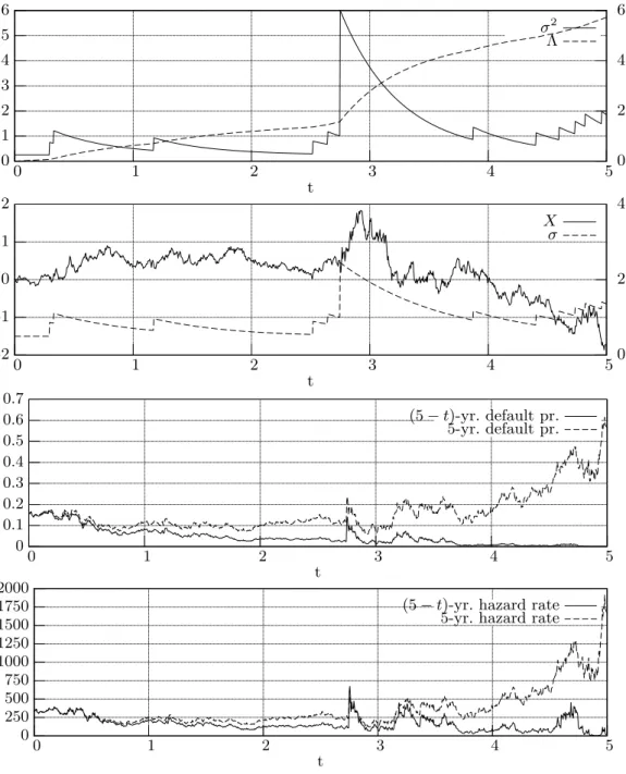
Equation (15) is verified by applying the Itˆo formula toeatσ2t (which establishesa fortiori that a solution to Equation (14) exists). The time-change increments is obtained by inte-grating each term of Equation (15). A sample path of σ2 and of Λ =R0tσs2ds is given in Figure 2.
3.5 Jumps in default probabilities and credit spreads
The continuity of the credit quality processX and the associated time-change Λ are crucial to derive the formula for conditional default probabilities, Equation (10), from which credit spreads can be computed. But recall that we wished to build a model that incorporates jumps in credit spreads. It turns out that for a credit quality process with the variance driven by an LOU process, jumps in the variance process propagate to default probabilities and credit spreads.
Proposition 3.6. Let X be a credit quality process with LOU variance process σ2 as in Proposition 3.5. Let τ = inf{t >0 :Xt≤b} be the associated default time. Fix T >0 and
let(P(t, T))t≤T be the associated conditional default probability process. Then, forP-almost
allω∈ {τ > t}, (P(t, T))t≤T is a process whose jumps are positive and
∆σt2(ω) = 0 ⇐⇒ ∆P(t, T)(ω) = 0, t < T.
A straightforward consequence of this Proposition is that a jump atσ2t triggers a jump in conditional default probabilitiesP(t, T), for all maturities T > t.
Proposition 3.7. Let (s(t, T))0≤t≤T be the CDS spread process for maturity T. Then
(s(t, T))0≤t≤T is c`adl`ag, and for t≤T and for P-almost all ω∈ {τ > t},
0 1 2 3 4 5 6 0 1 2 3 4 50 2 4 6 t σ2 Λ -2 -1 0 1 2 0 1 2 3 4 50 2 4 t X σ 0 0.1 0.2 0.3 0.4 0.5 0.6 0.7 0 1 2 3 4 5 t (5−t)-yr. default pr. 5-yr. default pr. 0 250 500 750 1000 1250 1500 1750 2000 0 1 2 3 4 5 t
(5−t)-yr. hazard rate 5-yr. hazard rate
Figure 2: Realization of variance process and credit quality process. Top: variance process
σ2, Equation (15) (continuous line, left axis); time-change Λ, Equation (16) (dashed line,
right axis). Second from top: credit quality processX, Equation (13) (continuous line, left axis); volatilityσ (dashed line, right axis). Second from bottom: 5-year default probability processP(t, T), Equation (11), with decaying time-to-maturity (continuous line) and with fixed time-to-maturity (dashed line). Bottom: Approximation of credit spreads(t, T) (term hazard rate, see Appendix A), with decaying time-to-maturity (continuous line) and with fixed time-to-maturity (dashed line).
Parameters: a = 2, θ ≡ 0.25, σ02 = 0.25; σ2 is driven by a compound Poisson process with jump intensityλ= 2 and discrete jump size distribution with jump sizes 0.05,5 with probabilities 0.95,0.05, respectively. The barrier isb=−3.
Consider the variance process in Figure 2: it has a large jump, which is also clearly visible in the default probability process and in the credit spread.
Note that the credit quality process model does not include events where credit spreads jump for selected maturities only. However, this is compatible with the observation that credit spreads tend to jump together, see Section 2.3.
Finally, it is easily seen that a jump in the variance process cannot lead to default P–a.s.. It suffices to observe that τ = inf{t > 0 : Xt ≤ b} is a predictable stopping
time, whereas the jumps of the driving compound Poisson process are totally inaccessible. However, we shall see later that jump-to-default events can be approximated by large jumps in the variance.
4
Computation of default probabilities and credit spreads
The implementation of the LOU variance model is a combination of Monte Carlo simulation and analytical computation. On {τ > t}, and conditional on Xt, σt2, default probabilities P(t, T) = P(τ ≤ T|Xt, σt2), T > t, can be computed numerically, so that Monte Carlosimulation reduces to simulating Xt and σ2t. The advantage of such an algorithm is that
valuation of a product involving P(t, T) or s(t, T) requires simulation only until t instead
of T. For example, to value a default swaption one needs to simulate merely until option
expiry instead of maturity of the underlying CDS (this will be treated in Section 7).
4.1 Jump size distribution of time-change Λ
Assume the credit quality process model (X, σ2) of Proposition 3.5, withσ2 a LOU process
driven by a compound Poisson process Z. We wish to compute conditional default
proba-bilities P(τ ≤T|Xt, σt), 0≤t≤T, according to Equation (11). Inspection of the formula
for the time-change increments ΛT −Λt, Equation (16), reveals that computation of the
conditional expectation (11) essentially entails computing the distribution of
Lt,T := X
t<u≤T
1−e−a(t−u)∆Zu.
Let Z have jump intensity λand jump size Y >0. For every t≤T, the random variable
Lt,T follows a compound Poisson distribution (see [Sato, 1999, Chapter 22] or [Norberg,
2004]),
Lt,T ∼CPO(λ(T −t),(1−e−a(T−S))Y), (17)
withS uniformly distributed on (t, T], i.e., S ∼U(t, T), and independent ofY. Moreover,
Lt,T L
=L0,T−t, hence it suffices to compute the distributions of LT := L0,T. The following
result states the distribution of the compounding variate (1−ea(T−S))Y of LT.
Lemma 4.1. For T >0, let S ∼ U(0, T) and let Y be a P–a.s. strictly positive random variable independent of S. The distribution of 1−ea(T−S)
Y is given by F(x) =E −ln(1−x/Y) aT 1{[0,1−e−aT)}(x/Y) +P Y ≤ x 1−e−aT , x∈R. (18) Proof. Conditioning under Y yields
F(x) =P1−e−a(T−S)Y ≤x=E P1−e−a(T−S)Y ≤x Y . (19)
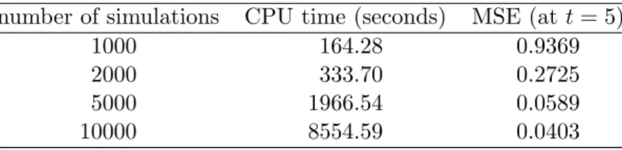
number of simulations CPU time (seconds) MSE (att= 5)
1000 164.28 0.9369
2000 333.70 0.2725
5000 1966.54 0.0589
10000 8554.59 0.0403
Table 1: Monte Carlo simulation vs. Panjer recursion. CPU time (Panjer recursion): 331.33 CPU secs.
Define gx(y) := P 1−e−a(T−S)
y≤x, y > 0. By the independence of S and Y, the conditional probability of Equation (19) is given bygx(Y). Since S∈[0, T],
gx(y) = 0, x≤0, 1, x≥(1−e−aT)y, −ln(1aT−x/y), x∈(0,(1−e−aT)y),
and the claim follows by inserting into Equation (19).
4.2 Panjer recursion
The distribution of LT can be computed efficiently using Panjer recursion, see [Panjer,
1981] or [McNeil et al., 2005, Chapter 10]. This method is based on a recursive evaluation formula for a family of compound distributions. In our implementation it has proven to be numerically more stable to assume a discrete distribution of the compounding variate, although the distribution function of the compounding variate in Equation (18) is
con-tinuous. For the compound Poisson case, the method works as follows: Suppose N is a
Poisson distributed random variable with intensity λ and let the compounding variate Y
take values in the nonnegative integers. Set f(i) =P(Y =i), i= 1,2, . . .. For a random variableL∼CPO(λ, Y), its distribution g(i) =P(L=i),i= 1,2, . . ., is given by
g(i) =
i X
n=0
fn∗(i)P(N =n), i= 1,2, . . . ,
wherefn∗(i) denotes then-fold convolution product off ati. The number of computations required for determiningg(i) is of the order i2. The result by Panjer states that
g(i) = λ i i X j=1 j f(j)g(i−j), i= 1,2, . . . ,
in which case the number of computations required for determiningg(i) is of the orderi. By proper scaling on an equidistant grid, the method can also be used for discrete nonnegative compounding variates not restricted to integers.
To illustrate the pickup in computational speed using Panjer recursion, we compare the computation of the distributions of Λti, with ti = i/10, i = 0, . . . ,200, for points x = (xi)i=0,...,8000, using Monte Carlo simulation and Panjer recursion. For the Monte
Carlo simulation, Λt was simulated at 200 time points with 8000 grid points each, with
1000, 2000, 5000 and 10000 simulations. The CPU times of the simulations are given in Table 1. In addition, the simulation results are compared with the computation using Panjer recursion by considering the simulation mean square error (MSE) relative to the value obtained by Panjer recursion.
Require: t1= 0< . . . < tN // time grid Require: x1= 0< . . . < xM // space grid Require: u1, . . . , uJ // desired maturities Require: K // number of simulations
Require: b // default barrier
Require: a,θ,λ,σ20,F // volatility process parameters,F jump size distribution
1: // Panjer recursion 2: fori= 1 toN do 3: forj= 1 toJ do 4: computeP(Lti∈[xj−1, xj)) 5: end for 6: end for 7: // simulation step 8: fork= 1 toK do
9: τk← ∞ // default time ofk-th simulation
10: forj= 1 toJ do
11: simulateσk
uj andX
k uj
12: sampled←1{minuj−1<s≤ujXs≤b}cond. onXuj−1 andXuj // (see text)
13: if d= 1 orXk uj ≤bthen 14: τk←u j 15: Pk(u j, uj+ti)←1,sk(uj, ti)←0 // for alli= 1, . . . , N
16: nextk // exitk-th simulation
17: end if 18: fori= 1 toN do 19: h←(1−e−ati)σ2 uj/a+ Ruj+ti uj θ(r) 1−e −a(uj+ti−r)dr 20: Pk(u j, uj+ti)←2P M m=1N b−Xuj √ h+xm−1/a P(Lti ∈[xm−1, xm)) 21: sk(uj, uj+ti)← −(1−R) ln(1−P(uj, uj+ti))/ti // credit triangle 22: end for 23: end for 24: end for
Algorithm 1: Computation of conditional default probabilities
4.3 Algorithm
Suppose we wish to compute default probabilitiesP(uj, uj+ti),j= 1, . . . J,i= 1, . . . , N.4
The full simulation algorithm, outlined below, is given in pseudo-code in Algorithm 1. For each ti, we compute the distribution of Lti on an equidistant space grid x1, . . . , xM.
Next, we simulateK paths of (σ, X), yielding (σuj)kj=1,...,J and (Xuj)kj=1,...,J,k= 1, . . . , K.
For each uj, we check if default has occurred. However, simulating on a discrete time
grid underestimates the occurrence of the default event. Hence, in addition we sample an indicator variable that determines whether default has occurred between two time points. This is realised by applying a well-known result to determine the barrier hitting event of
a Brownian bridge. Taking into account that X is a Brownian motion with a continuous
time-change, the indicator takes value 1 with probability e−2(b−Xuj−1)(b−Xuj)/(Λuj−Λuj−1), j= 2, . . . J, cf. [Glasserman, 2004, Section 6.4]. For each time pointuj and time-to-maturity ti, we determine Λti+uj−Λuj by computing the deterministic part and then the expectation
using the distributionLti.5 In this way we obtain a term structure of default probabilities,
which serves as the basis for computing credit spreads according to Equation (1). In the algorithm we use the credit triangle (see Appendix A) compute credit spreads.
4
For notational simplicity we compute anr×nmatrix of default probabilities; other setups of time points and time-to-maturities are possible.
5
Actually, the deterministic part need not be computed for every simulation, hence for efficiency the computation of Line 19 should take place outside the loopk= 1, . . . , K.
5
Calibration
Calibration is the process of assigning the parameters of the model such that the model reproduces market prices. One set of market prices is the term structure of credit spreads (or default probabilities). Further market prices, such as prices of default swaptions, provided they are available and liquid, may be suitable for calibrating the dynamics. In the absence of a liquid market for such claims, calibrating the dynamics via historical data may be a feasible alternative. We focus here on calibration to a given term structure and illustrate the attainable range of dynamics in the following section.
In the LOU model of Proposition 3.5, the deterministic functionθ and the initial
vari-ance σ02 will be chosen to reproduce a given term structure. The remaining parameters –
mean reversion constanta, jump intensityλ, jump size distributionF, barrierb– are chosen
to determine the dynamics. It should be noted, however, that the deterministic function θ
influences the dynamics and that the parameters for the dynamics influence the calibration ofθ. It is also the case that calibration to a given term structure imposes some restrictions on the dynamics parameters – in other words, given a set of dynamics parameters, it is not possible to achieve satisfactory calibration to an arbitrary term structure; this is outlined in detail below. The overall calibration process is to assign parameters for the dynamics first and then to calibrate to the spot curve.
The allocation of the parameters to spot curve calibration and dynamics calibration is justified as follows: in a model with a jump intensity of zero, the resulting time-change process is deterministic, which corresponds to the Overbeck-Schmidt model. In this case, the only parameters that are relevant for calibration to a given spot curve are the initial varianceσ2
0 and the deterministic functionθ, and the dynamics are fixed by the deterministic
time-change. Only when the jump intensity is greater than zero do the dynamics change, in which case all parameters allocated to the dynamics calibration become relevant for the dynamics.
5.1 Calibration to a term structure of default probabilities
Assume given a set of default probabilities P(Ti) := P(τ ≤ Ti), T1 < · · · < Tn, derived
from market-given credit spreads (together with a recovery assumption). For fixed mean reversion a, barrier b, jump intensity λ and jump size distribution F, the objective is to determineσ20 and θto match the given default probabilities. Since default probabilities in the LOU-model are expectations, cf. Equation (10), there is in general no analytic method to calibrate. Moreover, it turns out that it is not even guaranteed that an exact solution of the calibration problem exists. We require thatP(t, T),T ≥t, be strictly increasing, capturing the fact that a risky entity may default at any time, for every t≥ 0, P–a.s.. Clearly, by inspection of Equation (10), this condition is met if the time-change Λ is strictly increasing P–a.s., or, equivalently, ifσ2t >0,t≥0,P–a.s..
Although an exact solution to the calibration problem with a certain set of dynamics parameters may not exist, satisfactory calibration quality to a given term-structure may always be obtained. Indeed, a model without jump component is equivalent to the OS-model, where analytic and exact calibration is possible. By choosing suitably moderate jump dynamics, an arbitrary calibration quality may be achieved, as we shall see below.
We calibrate numerically by minimising the error between market-given and model-computed default probabilities. In the following, we shall always assumeθ to be piecewise constant, θ(t) = n X i=1 θ(Ti)1(Ti−1,Ti](t), t >0, (20)
default probabilities and model default probabilities as δ(σ02, θ;P, a, b, λ, F) := v u u t n X i=1 Ti−Ti−1 Tn P(Ti)−2EN b/pΛTi 2 , (21)
where the expectation denotes the model-given default probability for maturity Ti, cf.
Equation (12) and ΛTi is given by (cf. Equation (16))
ΛTi = 1−e−a Ti) σ2 0 a + i X j=1 θ(j) " Tj −Tj−1− e−a(t−Tj)−e−a(t−Tj−1) a # + 1 a X 0<u≤Ti 1−e−a(Ti−u) ∆Zu. (22)
In order for P(t, T), T ≥ t, to be strictly increasing for all t, we require that (cf. Equa-tion (15)) σt2=e−atσ02+ n X i=1 θ(Ti)e−at ea(t∧Ti)−ea(t∧Ti−1)+ X 0<u≤t e−a(t−u)∆Zu>0, t≥0.
Taking into account that jumps are positive, the condition is satisfied ifθsatisfies
θ(Ti)>−
σ02+Pi−1
j=1θ(Tj) eaTj−eaTj−1
eaTi−eaTi−1 , i= 1, . . . , n. (23)
Define the set
Θ ={(θ(T1), . . . , θ(Tn))∈Rn: (θ(T1), . . . , θ(Tn)) satisfies (23)}.
For the model-given probabilities to be well-defined requires additionally thatλ≥0,a >0,
b≤0 andF(0) = 0. Under these conditions, the solution to the calibration problem is then given by
(σ?02, θ?(T1), . . . , θ?(Tn)) := arg min
{σ2
0∈R+,(θ(T1),...,θ(Tn))∈Θ}
δ(σ02, θ;P, a, b, λ, F). (24)
Example 5.1. Assume given default probabilites P(Ti) = 1−e−hTi, at times Ti = i
(years),i= 1, . . . ,10, withh= 0.03. We calibrate the model to these default probabilities, for different jump size distributions, jump intensitiesλand mean reversion constantsa.
The distribution of L0,Ti, i = 1, . . . ,10, is computed on an equidistant grid of 5000
points in the interval [0,120]. The barrier isb=−3. The mean reversionaand the jump intensity λare chosen from the set{1,2,3,5,10}and the following jump size distributions are considered:
(i) The jump size is 1/4. (ii) The jump size is 1/2.
(iii) The jump size distribution is exponential with parameterν= 4, i.e.,F(x) = 1−e−νx. (iv) The jump size is 0.1 with probability 0.95 and 20 with probability 0.05. Here, we enlarged the grid for computing the distributions of (L0,Ti)i=1,...,10to 11000 points on
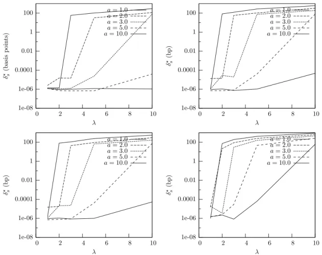
1e-08 1e-06 0.0001 0.01 1 100 0 2 4 6 8 10 δ ? s (b as is p oin ts ) λ a= 1.0 a= 2.0 a= 3.0 a= 5.0 a= 10.0 1e-08 1e-06 0.0001 0.01 1 100 0 2 4 6 8 10 δ ? s (b p) λ a= 1.0 a= 2.0 a= 3.0 a= 5.0 a= 10.0 1e-08 1e-06 0.0001 0.01 1 100 0 2 4 6 8 10 δ ? s (b p) λ a= 1.0 a= 2.0 a= 3.0 a= 5.0 a= 10.0 1e-08 1e-06 0.0001 0.01 1 100 0 2 4 6 8 10 δ ? s (b p) λ a= 1.0 a= 2.0 a= 3.0 a= 5.0 a= 10.0
Figure 3: RMSE’s of credit spreads for different parameter sets obtained by calibrating to default probabilities P(Ti) = 1−e−0.03Ti, i= 1, . . . ,10. Each figure contains six lines
that correspond to parameter a={1,2,3,5,10} (ordered from top to bottom at λ= 10). Top left, top right, bottom left and bottom right: jump size distribution as in (i)-(iv), respectively, of Example 5.1.
The RMSE’s for credit spreads, denoted by δs?, are given in Figure 3. Here, the spread (in basis points, 1bp = 0.01%) was computed from market-given default probabilities by
s(Ti) = 104·(1−R)
P(Ti) Pi
j=1(1−P(Tj))(Tj−Tj−1)
, i= 1, . . . , n,
and accordingly for model-given default probabilities. The recovery rate was R = 0.4.
Observe that for some parameter sets, the RMSE between market-given and model-given credit spreads is as small as 10−6. It turns out that the error is large when the jump intensity
λis high and mean reversion a is small. Increasing the frequency of jumps, increases the
volatility of the credit quality process, which in turn increases the likelihood of the credit quality process hitting the barrier. A too high jump intensity may thus inhibit satisfactory calibration to a given term structure. To understand the effect of a low mean reversion, one must study Equation (16). First of all, the jump size in the time-change Λ is scaled
by the mean reversion. Secondly, a low mean reversion “dampens” the function θ at the
short end of the term structure, which is then amplied for longer time-to-maturity. Thus, for low mean reversion, calibrating the short term default probabilities selects high values for θ, whose effect is intensified for long term default probabilities. It follows that under many circumstances a low mean reversion fails to calibrate well to either the short end or
5.2 Shape of credit-spread term structure
Examples of credit spread term structures with different parameters are given in Figure 4. Recall from the stylised empirical facts stated in Section 2.3 that a term structure of credit spreads may assume different shapes. Typically, an investment grade company’s term structure is upward sloping, reflecting lower default risk in the near future compared to higher uncertainty in the long term. A speculative-grade company may have an inverted term structure, indicating that the firm faces higher short-term default risk, but is more likely to survive in the long-term conditional on survival in the short-term.
A common observation is that credit spreads are strictly positive as time-to-maturity tends to zero, indicating that default may happen suddenly and unexpectedly. In Section 3.5 we established that the model is not capable of producing this property - credit spreads vanish as time-to-maturity tends to zero, and the default time is predictable. However, the possibility of large jumps in the variance may allow for “near-jump-to-default” events (see also case (d) of the examples presented in Section 6.1). We would then expect the spread term structure to be very steep at the short end.
By choosing extreme values for either the barrier or the initial variance, we obtain sharply humped term structures that approximate inverted term structures. Both cases reflect a low credit quality: default becomes more likely as either the credit quality process approaches the barrier or as the variance increases.
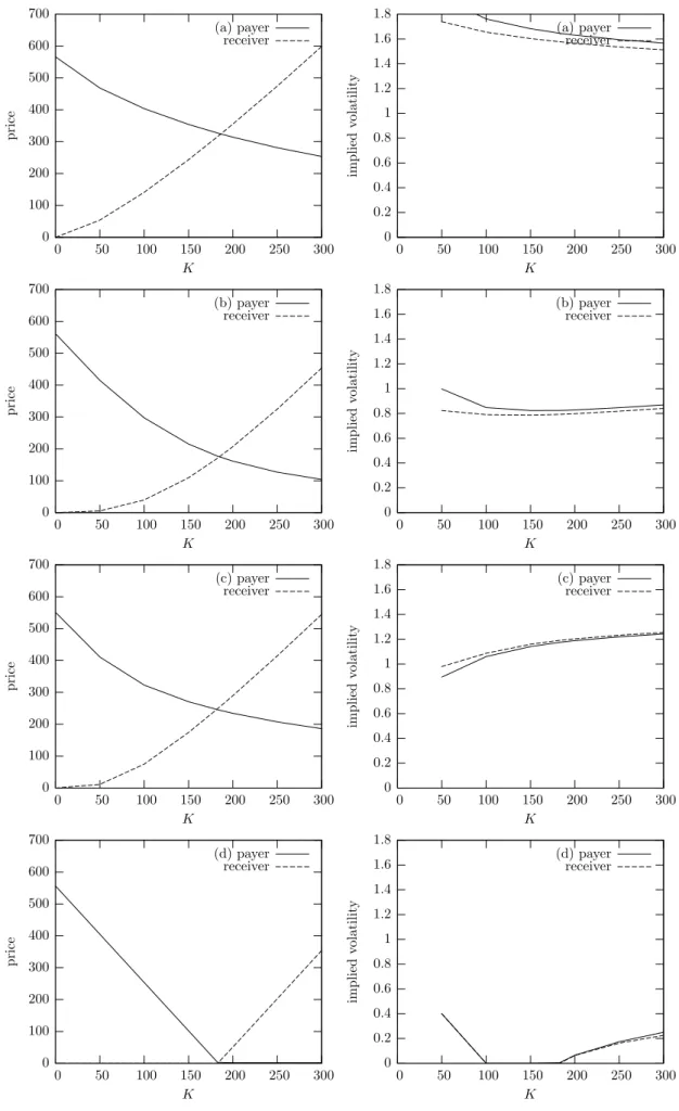
0 50 100 150 200 250 300 350 400 450 0 2 4 6 8 10 s (0 , T ) T a: 1.0 2.0 3.0 5.0 10.0 0 500 1000 1500 2000 2500 3000 3500 4000 4500 5000 0 2 4 6 8 10 s (0 , T ) T b:−1.0 −2.0 −3.0 −5.0 0 50 100 150 200 250 0 2 4 6 8 10 s (0 , T ) T pc:{0.925,0.075} {0.950,0.050} {0.975,0.025} {1.000,0.000} 0 100 200 300 400 500 600 700 0 2 4 6 8 10 s (0 , T ) T λ: 10.0 5.0 2.0 1.0 0 500 1000 1500 2000 2500 3000 0 2 4 6 8 10 s (0 , T ) T σ2 0: 20.0 5.0 1.0 0.1 0 100 200 300 400 500 600 700 800 900 0 2 4 6 8 10 s (0 , T ) T θ: 3.00 2.00 1.00 0.00
Figure 4: Impact of individual parameters on credit spread term structure. The standard parameter set is a = 3, b = −3, λ = 2, σ20 = 3, θ ≡ 0, jump size in {0.1,20} with probabilities {0.95,0.05}. pc denotes the jump size probabilities. In each case, the curves
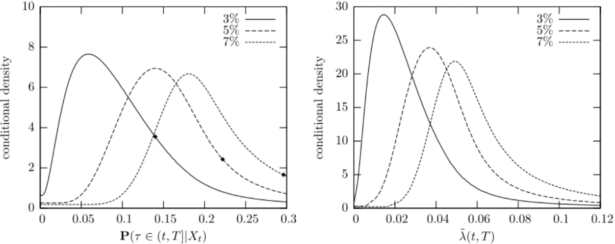
0 2 4 6 8 10 0 0.05 0.1 0.15 0.2 0.25 0.3 condi tional d e n si ty P(τ∈(t, T]|Xt) 3% 5% 7% 0 5 10 15 20 25 30 0 0.02 0.04 0.06 0.08 0.1 0.12 condi tional d e n si ty ˜ λ(t, T) 3% 5% 7%
Figure 5: Distributions ofP(t, T) (left) and ˜λ(t, T) (right) conditional on{τ > t}. The term hazard rate ˜λ(t, T) is an approximation of the credit spread, i.e.,s(t, T)≈(1−R)˜λ(t, T)·104
(in basis points). We have t = 1, T = 5 and initial hazard rates of 3%,5%,7%. The
diamonds mark the initial 5-year default probabilityP(τ ≤T). The model parameters are
mean reversion a= 3, recovery rate R = 0.4, barrier b = −3; σ2 is driven by compound
Poisson processes with jump intensity λ = 2 and jump size distributions {0.1,20} (h = 0.03), {0.2,50} (h = 0.05), {0.4,100} (h = 0.07) with probabilities {0.95,0.05}. In each
case, the the initial variance σ02 and the function θ were chosen to fit the given term
structure.
6
Dynamics
In general, the prices generated by the model should be consistent with any liquid market prices. For example, option prices, if available, provide a source of information for calibrat-ing risk-neutral dynamics. In the absence of such information, one may be forced to resort to information from historical time series.
6.1 Examples
To illustrate the range of dynamics, Figure 5 shows the distributions (conditional on no default) of the random variable P(τ ≤5|F1), i.e., of the 5-year default probability in one
year, for four different parameter sets, and the corresponding corresponding credit spread approximations (term hazard rates, see Appendix A). The parameters are given in Table 2. In each case, the initial varianceσ20 and the function θ are calibrated to match default probabilities corresponding to an initial hazard rate of 3%. For details on calculating the distribution of the random variableP(τ ≤T|Ft) see [Packham et al., 2009].
Case (a) is a model with a deterministic time-change, and hence corresponds to the
OS-model. Case (d) was chosen such that σ20 = 10−6 and θ ≡ 0, so that the variance is
very small until the first jump occurs. The jump size was chosen to be very large relative to the default barrier so that, heuristically, a single jump leads to default very quickly. Loosely speaking, case (d) can be considered an approximation of a reduced-form model with a deterministic and constant intensity: the credit quality process exhibits practically no movement, until the first jump occurs, which leads to default. This is also reflected in the jump intensity λ = 0.0305, which is approximately the initial hazard rate, and in P(τ ∈(1,5)|X1, σ12)≈1−e−0.03·4 = 0.11308 conditional on no default until time 1.6 These 6If the initial hazard rate is not constant, then a calibration where the variance moves purely by jumps
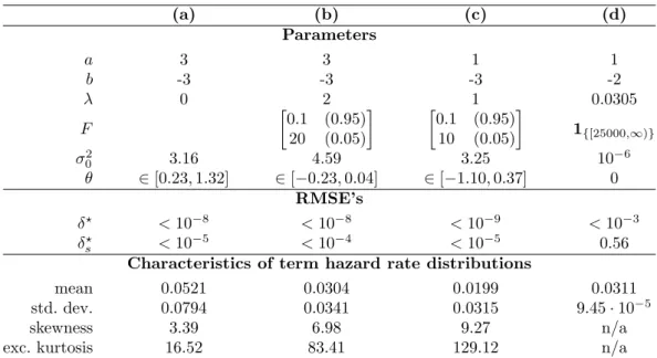
(a) (b) (c) (d) Parameters a 3 3 1 1 b -3 -3 -3 -2 λ 0 2 1 0.0305 F 0.1 (0.95) 20 (0.05) 0.1 (0.95) 10 (0.05) 1{[25000,∞)} σ2 0 3.16 4.59 3.25 10−6 θ ∈[0.23,1.32] ∈[−0.23,0.04] ∈[−1.10,0.37] 0 RMSE’s δ? <10−8 <10−8 <10−9 <10−3 δ? s <10−5 <10−4 <10−5 0.56 Characteristics of term hazard rate distributions
mean 0.0521 0.0304 0.0199 0.0311
std. dev. 0.0794 0.0341 0.0315 9.45·10−5
skewness 3.39 6.98 9.27 n/a
exc. kurtosis 16.52 83.41 129.12 n/a
Table 2: Parameters of dynamics examples. The jump sizes are given by the first column and the corresponding probabilities in the second column of each matrix in the row of parameterF.
two cases illustrate that the parameters can be classified into parameters that govern the jump part of the variance process, namely the jump intensity and jump size distribution, and parameters that control the continuous behaviour of the process in the sense that the level of the functionθdetermines the minimum “default speed” of the credit quality process at any time. By calibration to a term structure, a low level of jump activity leads to a higher minimum “default speed” and vice versa.
The characteristics of cases (b) and (c) are “in-between” cases (a) and (d): in both cases, the variance process exhibits jumps. However, the jump dynamics are moderate enough for the level of the variance process induced by θ and σ2
0, both of which are obtained by
calibration to the given term structure, to be significantly above zero. In other words, the variance processes of both cases feature jumps and a significant minimum “default speed”.
6.2 Parameters and dynamics
We discuss each parameter that influences the dynamics. These are the parameters of the variance process, i.e., mean reversion a, jump intensity λ, jump size distribution F, initial varianceσ2
0 and deterministic functionθ. Additionally, as will be outlined below, we
include the barrier b in our discussion. The initial variance σ02 and deterministic function
θ, although determined by calibration to a given term structure, influence the dynamics,
implying that the choice of dynamics and the calibration to the spot term structure cannot be separated.
Mean reversiona The mean reversion parameteradetermines the “speed” at which the variance reverts to its mean, cf. Equation (14). As can be seen from Equation (16) (resp. Equation (22)), the initial variance and jump size are scaled by 1/a. Additionally, the factors (1−e−aT) and (1−e−a(T−u)) “dampen” the impact ofθandZ for short maturities, which are then amplified for longer maturities. The smaller a is chosen, the stronger this
cannot be attained. This is due to the fact that the jump intensity of the variance’s compound Poisson process is constant, whereas a non-constant, deterministic hazard rate requires the jump intensity to be non-constant and deterministic. The former can be incorporated by specifying the jump process as an additive process, which is more general than a L´evy process.
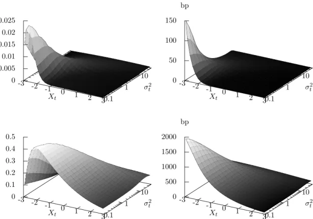
-3 -2 -1 0 1 2 3 Xt 0.1 1 10 σ2t 0 0.005 0.01 0.015 0.02 0.025 -3 -2 -1 0 1 2 3 Xt 0.1 1 10 σ2t 0 50 100 150 bp -3 -2 -1 0 1 2 3 Xt 0.1 1 10 σ2t 0 0.1 0.2 0.3 0.4 0.5 -3 -2 -1 0 1 2 3 Xt 0.1 1 10 σ2t 0 500 1000 1500 2000 bp
Figure 6: Jump size of 5-year default probability (left) and credit spread (right) when a
jump of size 0.1 (top), resp. 20 (bottom) occurs. Parameters correspond to case (b) of
Table 2.
effect of amplification as maturity increases. As outlined in Section 5.1, a small value of
afrequently leads to poor calibration: Large values of θ are determined for a satisfactory calibration at the short end, which are then too large for a proper calibration to longer maturities. On the other hand, a small mean reversion makes the impact of jumps in the variance process more long-lasting.
Barrier b Strictly speaking, the inclusion of the barrier as a parameter is redundant:
For any two barriersb and b0 we may obtain the same spot curve and dynamics by proper
scaling ofσ02,θand the jump size. On the other hand, one can see in Figure 4 that a change in the barrier affects the shape of the curve. To obtain the desired shape, it may be more straightforward to adjust the barrier instead of adjusting the set of other parameters. Jump intensity λ and jump size distribution F The jump intensity determines the average number of jumps to occur per year. The results from Section 3.5 imply that the jump intensities of the variance process and the term structures of default probabilities and credit spreads are all equal. The jump size ofZ propagates to the credit spread jump size
in a monotone way: the larger the jump of Z, the larger the jump in the credit spread –
this is easily seen by the by monotonicity of default probabilities in σ2 and extended to
credit spreads via the CDS valuation formula (1).
However, the jump size also depends on the level ofX andσ2. For default probabilities,
t there is a jump, ∆σ2t > 0. For any maturity T > t, limXt↓b∆P(t, T) = 0, as the
jump size is bounded by 1−P(t−, T) and limXt↓bP(t−, T) = 1. On the other hand,
limXt↑∞∆P(t, T) = 0 since ∆σt2 < ∞ P–a.s.. By Proposition 3.6, ∆P(t, T) > 0 for any
fixedXt, so ∆P(t, T) cannot be monotone inXt.
For credit spreads, the situation is not so clear. Examples indicate that the jump size
of credit spreads is monotone in X; Figure 6 provides an example of the jump size as a
function ofXt and σt2.
Initial variance σ02 and deterministic function θ Although σ02 and θ are chosen by calibration to a given term structure, their effect on the dynamics are significant. Intuitively, a decrease in the L´evy measure ofZ(i.e., decrease in jump intensity or jump size), decreases the probability of default, which is compensated by a higher choice of θ when calibrating. Consequently, the variance process will maintain a higher deterministic level, causing the credit quality process to evolve in a more volatile fashion in order to hit the default barrier with a certain probability. This is well illustrated by comparing cases (a) and (d) of the previous example, Section 6.1.
6.3 Evolution of the term structure shape
In Section 5.2 it was shown that the shape of the term structure becomes inverted (more precise: sharply humped) with increasing barrier band with increasing initial varianceσ02, cf. Figure 4. By inspection of the formula for conditional default probabilities we see that default probabilities at timetdepend on the distance-to-defaultb−Xt. Both a decreasing
distance-to-default and an increasing variance imply a decrease in credit quality, which eventually results in an inverted credit spread term structure.
7
Valuation examples
7.1 Information flow and pricing filtration
So far, we have made no assumptions about the filtration (Ft)t≥0, other than that it is rich
enough for the credit quality process (X, σ2) to be (Ft)t≥0-adapted. For a market model to
be consistent with arbitrage theory requires that the filtration used for pricing is generated by observable information. For building trading strategies, the underlying filtration must even be generated by the observable prices of traded assets, see e.g. Chapter 7 of [Hunt and Kennedy, 2004]. In general, a credit quality process (X, σ2) is neither directly observable nor a traded asset.
Suppose now that we wish to price financial claims derived from credit spreads (or, equivalently, default, resp. survival probabilities). Application of a risk-neutral valuation formula with conditional default probabilities given by the model via Equation (10) (or credit spreads derived thereof) is justified only if (Ft)t≥0 is generated by some observable
information and if X and σ2 are (Ft)t≥0-adapted. Otherwise, valuation of assets requires
that prices are computed using a different – possibly coarser – filtration. One may think of a coarser filtration as the inavailability in the market of complete information about a company’s state.
Assuming independence of risk-free interest rates and the default indicator process, the filtration generated by risk-free zero-coupon bonds (B(t, T))T≥t and conditional default
probabilities (P(t, T))T≥t, t≥0, will be sufficient for this purpose; owing to the valuation
formula for risky zero-coupon bonds, given by E e−RtTrsds1{ τ >T}|Ft =B(t, T)P(τ > T|Ft), T ≥t,
this filtration is equivalent to the filtration generated by risk-free and risky zero-coupon bonds (of all maturities).
The assumption that there is indeed a process that drives a company’s credit quality via the information available about the company may be justified by the stylised facts recorded earlier, namely that the arrival of news about a company affects CDS spreads of all maturities in a similar fashion. We shall assume that the credit quality of a firm is indeed driven by a process (X, σ2) as in Proposition 3.5 with σ2 an LOU process driven
by a compound Poisson process (with respect to the filtration (Ft)t≥0). Furthermore, we
assume that the parameters of the credit quality process are known, i.e., θ,σ20, a,b, c, λ,
F are F0-measurable. The following result establishes that, under these assumptions, the
formula for conditional default probabilities is suitable for valuation.
Proposition 7.1. Let (X, σ2) be a credit quality process as in Proposition 3.5, withσ2 an LOU process driven by a compound Poisson process. Let FP
t =σ((P(s, T)T >s),0≤s≤t).
Then,σ(Xt, σt2)⊆ FtP. Moreover, P(τ ≤T|FtP) =P(τ ≤T|Xt, σt2).
For the proof see [Packham et al., 2009].
7.2 Leveraged credit-linked note
As an example application of the model we value a leveraged credit-linked note using the pricing formula (3), with pricing done via Algorithm 1. The note has a maturity of 5 years
and a notional amount of e100. The leverage factor is k = 5, so that the payoff amount
and time are linked to the mark-to-market value of a CDS position with nominale500 on
CDS with a maturity of 5 years at inception. The trigger level is K = e60. The initial
CDS spread term structure is flat at 180 basis point, the recovery rate is 40%. The note is monitored weekly, i.e., at time points t1 < t2 < · · · < t260, with ∆ti = 1/52. Denote
by Vtk the mark-to-market value at time t of the CDS position. The note is unwound at
S = inf{ti : Vtik ≤ −K, i = 1, . . . ,260}. At S, the investor receives max(e100 +VSk,0)
and the issuer pays max(−VSk−e100,0) (the gap option payoff). The premium of the gap option is (k−˜k)s(0, T). The risk-free interest rate is constant at 5%.
For each dynamics example we generated 10 times 1000 simulations. From each batch of 1000 simulations, we computed the fair factor ˜k, the spread (k−˜k)s(0, T) (the total of which, over the lifetime of the note, is the gap option premium, cf. Equation (4)) and the spread on the note (for the investor) sinv = ˜ks(0, T) for each of the four example
models exhibiting different dynamics from Section 6.1. Additionally, denoting byLinv the
discounted loss to the investor, we computed the expected lossE(Linv), the probability that
a loss occurs, the probability of a total lossLinv,tot, the expected discounted earnings from
the spread payments (excluding the default-free interest of the coupon payment), E(Einv),
and the expected trigger time S conditional on a trigger event. The values obtained are
given in Table 3; here, each table entry consists of the mean value taken over all runs and (in parentheses) the standard deviation with respect to the 10 simulation runs (the 10 simulation scenarios are simulations of the estimator, each of which is approximately normally distributed by the usual Central Limit Theorem).
Recall that in Section 2.4 we already determined the fair factor ˜k for some models
via no-arbitrage arguments. Specifically, in the case where the mark-to-market value of a CDS evolves continuously, and when there is no jump-to-default risk, the fair factor is ˜
k = k, as there is no gap risk involved. This corresponds to case (a). Now consider the
case where the mark-to-market value is constant and the note is exposed to default risk only by a jump-to-default event. Then ˜k= 1/(1−R) as the investor’s payoff is equivalent to selling protection on 1/(1−R) CDS. This corresponds to case (d). Here, ˜k is slightly larger than 1/(1−R) = 1.67 as there is still some, albeit small, volatility that drives