Recognizing textual entailment using deep learning techniques

(1)

Recognizing Textual Entailment using

Deep Learning Techniques

Master Thesis Project

Master in Innovation and Research in Informatics

– Data Mining and Business Intelligence

Han Yang

Supervisor:

Marta R. Costa-jussà

Department of Signal Theory and

Communications

Tutor:

Lluí

s Padró Cirera

Department of Computer Science

FACULTAT D’INFORMÀTICA DE BARCELONA (FIB)

UNIVERSITAT POLITÈCNICA DE CATALUNYA (UPC) – BARCELONATECH

(2)

Acknowledgment

I would like to thank my supervisor Marta R. Costa-jussà

for her guidance and patience throughout

the whole development and writing process of this thesis.

Also to my family and my girlfriend X. Yu,

who have been very supportive and kept me up

(3)

Abstract

Textual Entailment (TE) or Natural Language Inference (NLI) refers to the problem of determining a directional relation between two text fragments. To specify, given a sentence pair (a, b), the task is to predict whether b is entailed by a, b is contradicted to a, or whether the relation between a and b is neutral.

NLI is a central problem in natural language understanding. Recently, the dominating trend of works for NLI is based on artificial neural networks, which aims at building deep and complex encoder to transform a sentence into encoded vectors. End-to-end artificial neural networks have reached state-of-the-art performance in NLI field. For instance, there are recurrent neural network based encoders, which recursively concatenate each word with its previous memory, until the whole information of a sentence has been derived. The most common RNN encoders are Long Short-Term Memory Networks (LSTM; Hochreiter and Schmidhuber, 1997) and Gated Recurrent Unit (Cho et al., 2014). RNNs have surpassed the performance of traditional baselines in many NLP tasks (Dai et al., 2015). There are also convolutional neural network (LeCun et al., 1989) based encoders, which concatenate the sentence information by applying multiple convolving filters over the sentence. CNNs have achieved state-of-the-art results on computer vision (Krizhevsky et al., 2012), machine translation (Costa-jussà M.R., 2016) and also on various NLP tasks (Collobert et al., 2011).

In this paper, we use the model introduced by (Adina Williams et al., 2017) as the baseline model for the NLI task. The baseline model is consisted with a word-level embedding layer and a BiLSTM encoder. We augment the baseline model and propose our Character-level Intra Attention Networks (CIAN). In our CIAN model, we use the character-level convolutional network to replace the standard word-level embedding layer, and we use the intra attention layer to capture the intra-sentence semantics. One contribution of our CIAN model is that we implement the character-level convolutional network introduced by (Kim et al., 2016). Most of the sequence encoders use word-level embedding layer initialized with pre-trained word vectors such as GloVe (Pennington et al., 2014). In that way, the words in a sentence are not independent anymore, which helps the encoders to catch more internal information of a sentence. However, as the growth of vocabulary size in the modern corpus, there will be more and more out-of-vocabulary (OOV) words that are not presented in the pre-trained word embedding vector. As the word-level embedding is blind to subword information (e.g. morphemes), it leads to high perplexities for those OOV words. We use the character-level convolutional network in our model to exploit the character-level information, which will be computed from the characters of corresponding word. By doing so, our model gains the ability to learn rich semantic and orthographic features from the encoding of characters.

Another contribution of our CIAN model is that we implement the intra attention mechanism introduced by (Z. Yang et al., 2017). The major advantage of attention mechanism is the ability to efficiently encode

(4)

and precision if they only use the final representation. Attention is a clever way to fix this issue and experiments indeed confirm the intuition. Another advantage of attention mechanism is that we can enhance the interpretability of the model by visualizing the attention weights of an encoded sentence. We conduct the visualization of the attention weights in chapter 5, which helps us to understand how the model judges the textual entailment relation between two sentences.

The proposed CIAN is implemented using Keras and evaluated upon a newly published MNLI corpus in the RepEval 2017 workshop. The test accuracy for the CIAN model upon matched test dataset is improved with 0.9 percent compared with the baseline model. Based on the improved result, we published a paper with title Character-level Intra Attention Networks for Natural Language Inference

in the RepEval 2017 workshop, as an achievement of this thesis.

To summarize, the CIAN model presented in this paper is a sequence encoder that has the ability to to encode long sentence in character-level with rich semantic and orthographic features. Also, the attention mechanism provides high interpretability of the model that allows people to understand how the model doing its task. As it’s an end-to-end neural network that does not need any specific pre-processing or outside data like pre-trained word embeddings. It can be easily applied to other encoder architecture tasks such as language modeling, sentiment analysis and question answering.

Key words: textual entailment, natural language inference, deep learning, sequence encoder, character-level encoder, attention mechanism

(5)

Introduction

1.1. Overview

1.1.1. Natural Language Inference

Natural language inference (NLI) or Textual Entailment (TE) in natural language processing refers to the problem of determining a directional relation between two text fragments. The relation holds whenever the truth of one text fragment follows from another text. In the NLI framework, the entailing and entailed texts are termed as premise and hypothesis.

The main task in this thesis does the textual entailment as a three-way classification. Given a sentence pair (a, b), the task is to predict whether b is entailed by a, b is contradicted to a, or whether the relation between a and b is neutral.

Here is some examples of the NLI task:

Premise Hypothesis Relation

A soccer game with multiple males playing.

Some men are playing a sport. Entailment

A black race car starts up in front of a crowd of people.

A man is driving down a lonely road. Contradiction

A smiling costumed woman is holding an umbrella.

A happy woman in a fairy costume holds an umbrella.

Neutral

Table 1: Examples of natural language inference task

1.1.2. Deep Learning

Recently, the dominating trend of works in natural language processing is based on artificial neural networks, which aims at building deep and complex encoder to transform a sentence into encoded vectors. Those kinds of neural networks that convert the input data into different representation vectors is called an encoder. The encoder is trained to preserve as much information as possible when an input

(8)

For instance, there are recurrent neural network (RNN) based encoders, which recursively concatenate each word with its previous memory, until the whole information of a sentence has been derived. The most common RNN encoders are Long Short-Term Memory Networks (LSTM; Hochreiter and Schmidhuber, 1997) and Gated Recurrent Unit (Cho et al., 2014). RNNs have surpassed the performance of traditional baselines in many NLP tasks (Dai et al., 2015).

There are also convolutional neural network (CNN; LeCun et al., 1989) based encoders, which concatenate the sentence information by applying multiple convolving filters over the sentence. CNNs have achieved state-of-the-art results on computer vision (Krizhevsky et al., 2012), machine translation (Costa-jussà M.R., 2016) and also on various NLP tasks (Collobert et al., 2011).

Deep learning as a particular kind of machine learning, achieves great power and flexibility by learning to represent the world as a nested hierarchy of concepts and representations. In this thesis, we will use the power of deep learning to handle the task for natural language inference.

1.1.3. RepEval2017 shared task

1

To evaluate the quality of various NLI models, the Stanford Natural Language Inference (SNLI) corpus of 570K sentence pairs was introduced (Bowman et al., 2015). It serves as a standard benchmark for NLI task. However, most of the sentences in SNLI corpus are short and simple, which limit the room for fine-grained comparisons between models.

Currently, a more comprehensive Multi-Genre NLI (MNLI) corpus of 433K sentence pairs is released, aiming at evaluating large-scale NLI models (Adina Williams et al., 2017). Authors also give out some baseline results together with the publishment of the MNLI corpus, the BiLSTM model achieves an accuracy of 67.0%, and the Enhanced Sequential Inference Model (ESIM; Chen et al., 2017) achieves an accuracy of 72.4%. Together with the release of the corpus, there is a RepEval2017 workshop co-located with EMNLP 2017, aiming at evaluating the sequence encoder models upon the MNLI corpus. RepEval2017 workshop features a shared task meant to evaluate natural language inference models based on sentence encoders, that transform sentences into fixed-length vector representations and reason using those representations. The task will be a three-class balanced classification problem over sentence pairs upon MNLI corpus.

The main work of this master thesis is related with this RepEval2017 workshop shared task.

1_{https://repeval2017.github.io/}

(9)

1.2. Objectives and contributions

In this thesis, a deep neural network sentence encoder will be implemented to deal with the natural language inference task of RepEval2017 workshop. The BiLSTM model from (Adina Williams et al., 2017) will be used as the baseline model for the evaluation of the MNLI corpus.

To augment the baseline model, firstly, a character-level convolutional neural network introduced by (Kim et al., 2016) is applied. We use the character-level CNN to replace the word embedding layer in the baseline model, which will be computed from the characters of corresponding word. Secondly, the intra-sentence word attention mechanism introduced by (Z. Yang et al., 2017) will be applied, to enhance the model with a richer information of substructures of a sentence. We name the final augmented model as Character-level Intra Attention Networks (CIAN), which is the main contribution of this master thesis.

1.3. Organization

In the following chapters of this document, we will discuss the related backgrounds of the Character-level Intra Attention Networks (CIAN), then take a detailed walkthrough of CIAN, followed by some experiments and analysis.

Chapter 2 discusses the necessary background of this thesis, including the algorithms of the neural networks, the concept of sequence encoder and attention mechanism and the technical tools used in this thesis.

Chapter 3 show the state-of-the-art concept used in this thesis, including the character-level convolutional neural network and the attention mechanism.

Chapter 4 introduces the Character-level Intra Attention Networks (CIAN), which is the main contribution of this thesis. The augmented layers using the concepts in chapter 3 and some practical tricks during model implementation will be described.

Chapter 5 contains the evaluation of the CIAN model, which contains the experimental results upon the MultiNLI dataset and some conducted error analysis.

(10)

Chapter 2.

Background

2.1. Neural networks

In this section, we will discuss the basic concept of an artificial neural network, including a single layer feedforward neural network (multilayer perceptron), the objection function of the neural networks and how to train the network using backpropagation.

2.1.1. Artificial neural networks

Artificial neural networks (ANNs) or connectionist systems are a computational model used in machine learning, computer science and other research disciplines, which is based on a large collection of connected simple units called artificial neurons. Connections between neurons carry an activation signal of varying strength. If the combined incoming signals are strong enough, the neuron becomes activated and the signal travels to other neurons connected to it. Such systems can be trained from examples, rather than explicitly programmed, and performs well in areas where the solution or feature detection is difficult to express in a traditional computer program. Like other machine learning methods, neural networks have been used to solve a wide variety of tasks, like computer vision and speech recognition, that are difficult to solve using ordinary rule-based programming.

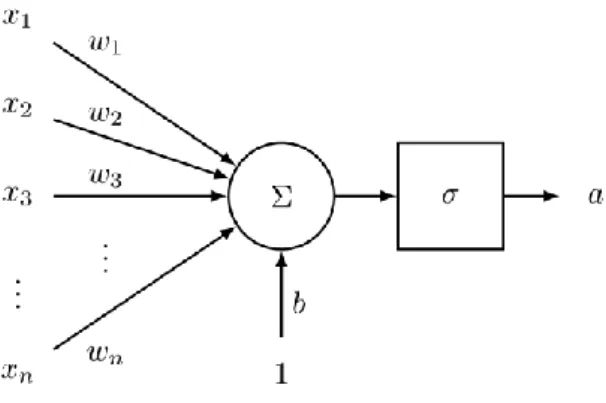
A neuron is a generic computational unit that takes n inputs and produces a single output. What differentiates the outputs of different neurons is their parameters (weights). One of the most popular choices for neurons is the "sigmoid" or "binary logistic regression" unit. This unit takes an n-dimensional input vector x and produces the scalar activation (output) a. This neuron is also associated with an n-dimensional weight vector, w, and a bias scalar, b. The output of this neuron is then:

α = 1

1 + exp⁡(−(𝜔𝑇_{𝑥 + 𝑏))} (1)

We can also combine the weights and bias term above to equivalently formula:

α = 1

1 + exp⁡(−[𝜔𝑇_{⁡⁡⁡𝑏] ∙ [𝑥⁡⁡⁡1])} (2)

(11)

Figure 1: A single neuron

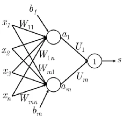
The idea above can be extended to multiple neurons by considering the case where the input x is fed as an input to multiple such neurons.

If we refer to the different neurons’ weights as { w(1)_{, … ,w}(m)_}_{and the biases as}_{{ b}

1, ... , bm }, we can say the respective activations are { a1, … , am }:

α1= 1 1 + exp⁡(−(𝜔(1)𝑇_{𝑥 + 𝑏} 1)) ⋮ α𝑚= 1 1 + exp⁡(−(𝜔(𝑚)𝑇_{𝑥 + 𝑏} 𝑚)) (3)

Let us define the following abstractions to keep the notation simple and useful for more complex networks: σ(z) = [ 1 1 + exp⁡(𝑧1) ⋮ 1 1 + exp⁡(𝑧𝑚)] b = [ 𝑏1 ⋮ 𝑏𝑚 ] W = [ − 𝜔(1)𝑇 ₋ … − 𝜔(1)𝑇 − ] (4) (5) (6)

We can now write the output of scaling and biases as:

z = 𝑊𝑥 + 𝑏 (7)

The activations of the sigmoid function can then be written as:

[ 𝛼1

⋮ 𝛼𝑚

(12)

We can think of these activations as indicators of the presence of some weighted combination of features. We can then use a combination of these activations to perform classification tasks. The following figure 2 captures how a simple feed-forward network might compute its output.

Figure 2: A simple feed-forward network

2.1.2. Objective Function

Like most machine learning models, neural networks also need an optimization objective, a measure of error or goodness which we want to minimize or maximize respectively. Here, we will discuss a error metric known as the maximum margin objective function.

If we call the score computed for the "true" labeled data as s and the score computed for the "false" labeled data as sc. Then, our objective function would be to maximize (s - sc) or to minimize (sc - s). However, we modify our objective to ensure that error is only computed if sc > s⇒(sc - s) > 0. The intuition behind doing this is that we only care the the "true" data point have a higher score than the "false" data point and that the rest does not matter. Thus, we want our error to be (sc - s) if sc > s else 0. Thus, our optimization objective J is now:

minimize⁡J = max⁡(𝑠𝑐− s, 0) 𝑠𝑐 = 𝑈𝑇𝑓(𝑊𝑥𝑐+ 𝑏) 𝑠 = 𝑈𝑇_{𝑓(𝑊𝑥 + 𝑏)} (9) (10) (11) However, the above optimization objective is risky in the sense that it does not attempt to create a margin of safety. We would want the "true" labeled data point to score higher than the "false" labeled data point by some positive margin 𝛥. In other words, we would want error to be calculated if (s - sc < ∆) and not just when (s - sc < 0). Thus, we modify the optimization objective J as follows:

minimize⁡J = max⁡(∆ + 𝑠𝑐− s, 0) (12)

We can scale this margin such that it is ∆ = 1 and let the other parameters in the optimization problem adapt to this without any change in performance. Finally, we define the following optimization objective which we optimize over all training windows:

(13)

2.1.3. Training: Backpropagation

In this section, we discuss how we train the parameters in a model using the cost function discussed in

section 2.1.2. Since we typically update parameters using gradient descent (or a variant such as SGD), we typically need the gradient information for any parameter as required in the update equation:

𝜃(𝑡+1)_{= 𝜃}(𝑡)_{− 𝛼∇𝜃}(𝑡)_𝐽 ₍₁₄₎

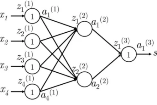
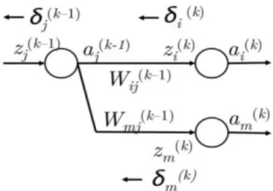
Backpropagation is technique that allows us to use the chain rule of differentiation to calculate loss gradients for any parameter used in the feed-forward computation on the model. To understand this further, let us understand the toy network shown in Figure 3 for which we will perform backpropagation.

Figure 3: A 4-2-1 neural network

Here, we use a neural network with a single hidden layer and a single unit output. Let us establish some notation that will make it easier to generalize this model later:

• xi is an input to the neural network. • s is the output of the neural network.

• Each layer (including the input and output layers) has neurons which receive an input and produce an output. The j-th neuron of layer k receives the scalar input zj(k)

and produces the scalar activation output aj(k) .

• We call the back propagated error calculated at zj(k) as δj(k) .

• Layer 1 refers to the input layer and not the first hidden layer. For the input layer, xj = zj(1) =

aj(1) .

• W(k)_{is the transfer matrix that maps the output from the k-th layer to the input to the}_(k+1)-th layer. Thus, W(1)₌_W_and_W(2)₌_U_{as perspective of}_{Section 2.1.1}_.

(14)

Figure 4: The subnetwork of figure 3 with weight matrix Wij

Suppose the cost J = (1 + sc - s) is positive and we want to perform the update of parameter W14(1) in Figure 4. We must realize that W14(1) only contributes to z1(2) and thus a1(2). This fact is crucial to understanding backpropagation – backpropagated gradients are only affected by values they contribute to. Thus, we can calculate error gradients with respect to a parameter in the network using the gradient chain rule.

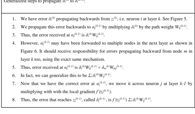
Following table 2 shows the generalized steps for backpropagation.

Generalized steps to propagate δi(k) to δi(k-1):

1. We have error δi(k) propagating backwards from zi(k), i.e. neuron i at layer k. See Figure 5. 2. We propagate this error backwards to αj(k-1) by multiplying δi(k) by the path weight Wij(k-1). 3. Thus, the error received at αj(k-1) is δi(k)Wij(k-1).

4. However, αj(k-1) may have been forwarded to multiple nodes in the next layer as shown in Figure 6. It should receive responsibility for errors propagating backward from node m in layer k too, using the exact same mechanism.

5. Thus, error received at αj(k-1) is δi(k)Wij(k-1) + δm(k)Wmj(k-1). 6. In fact, we can generalize this to be Σi δi(k)Wij(k-1).

7. Now that we have the correct error at αj(k-1), we move it across neuron j at layer k-1 by multiplying with with the local gradient f’(zj(k-1)).

8. Thus, the error that reaches zj(k-1), called δj(k-1) , is f’(zj(k-1)) Σi δi(k)Wij(k-1).

Table 2: Generalized steps of backpropagation

(15)

Figure 6: Propagating error from δi(k) to δi(k-1)of multiple nodes

So far, we discussed how to calculate gradients for a given parameter in the model. Here we will generalize the approach above so that we update weight matrices and bias vectors all at once. Note that these are simply extensions of the above model that will help build intuition for the way error propagation can be done at a matrix-vector level.

For a given parameter Wij(k), we identified that the error gradient is simply δi(k+1)⋅αj(k). Thus, we can write an entire matrix gradient using the outer product of the error vector propagating into the matrix and the activations forwarded by the matrix.

Now, we will see how we can calculate the error vector δ(k)_{. We established earlier using Figure 6 that}

δj(k) =f’(zj(k)) Σi δi(k+1)Wij(k). This can easily generalize to matrices such that:

𝛿(𝑘)_{= 𝑓}′_(𝑧(𝑘)_{) ∘ (𝑊}(𝑘)𝑇_)𝛿(𝑘+1) ₍₁₅₎

In the above formulation, the operator corresponds to an element wise product between elements of vectors (∘ : R N_{× R} N_{→ R}N₎_.

Having explored element-wise updates as well as vector-wise updates, we must realize that the vectorized implementations run substantially faster in scientific computing environments such as MATLAB or Python (using NumPy/SciPy packages). Thus, we should use vectorized implementation in practice. Furthermore, we should also reduce redundant calculations in backpropagation - for instance, notice that δ(k)_{depends directly on}_δ(k+1)_{. Thus, we should ensure that when we update}_W(k)_using_δ(k+1)_, we save δ(k+1)_{to later derive}_δ(k)_{– and we then repeat this for}_{(k - 1) . . . (1)}_{. Such a recursive procedure} is what makes backpropagation a computationally affordable procedure.

2.2. Sequence encoder

In this section, we will discuss two kinds of sequence encoders, the recurrent neural network encoder and the convolutional neural network encoder.

2.2.1. Recurrent neural network encoder

(16)

A recurrent neural network (RNN) is a class of artificial neural network where connections between units form a directed cycle. This creates an internal state of the network which allows it to exhibit dynamic temporal behavior. Unlike feedforward neural networks, RNNs can use their internal memory to process arbitrary sequences of inputs. This makes them applicable to tasks for the natural language processing field as the inputs to the network are sequences of words.

Figure 7: A Recurrent Neural Network

Figure 7 introduces the RNN architecture where rectangular box is a hidden layer at a time-step, t. Each such layer holds a number of neurons, each of which performing a linear matrix operation on its inputs followed by a non-linear operation (e.g. tanh()). At each time-step, the output of the previous step along with the next word vector in the document, xt, are inputs to the hidden layer to produce a prediction output ŷ and output features ht (Equations 16 and 17).

ht = σ(W (hh)_h

t-1 + W (hx)x[t])

ŷt = softmax(W(S)ht)

(16) (17) Below are the details associated with each parameter in the network:

● x1, ..., xt-1, xt, xt+1, …, xT: the word vectors corresponding to a corpus with T words. ● ht = σ(W (hh)_h

t-1 + W (hx)x[t]): the relationship to compute the hidden layer output features at each time-step t.

● ŷt = softmax(W(S)ht): the output probability distribution over the vocabulary at each time-step t. Essentially, ŷt is the next predicted word given the document context score so far (i.e. ht-1) and the last observed word vector x(t)_{. Here,}_W(S)_∊_R|V|Dh_and_ŷ_∊_R|V|_where_|V|_{is the vocabulary.} The loss function used in RNNs is often the cross-entropy error introduced in earlier notes. Equation below shows this function as the sum over the entire vocabulary at time-step t.

𝐽(𝑡)_{(𝜃) = − ∑ 𝑦} 𝑡,𝑗×⁡log(ŷ𝑡,𝑗) |𝑉| 𝑗=1 (18)

The cross-entropy error over a corpus of size T is:

𝐽 = −1 𝑇∑ 𝐽 (𝑡)_(𝜃) 𝑇 𝑡=1 = −1 𝑇∑ ∑ 𝑦𝑡,𝑗×⁡log(ŷ𝑡,𝑗) |𝑉| 𝑗=1 𝑇 𝑡=1 (19)

(17)

The amount of memory required to run a layer of RNN is proportional to the number of words in the corpus. For instance, a sentence with k words would have k word vectors to be stored in memory. Also, the RNN must maintain two pairs of W, b matrices. While the size of W could be very large, it does not scale with the size of the corpus. For a RNN with 1000 recurrent layers, the matrix would be 1000 × 1000 regardless of the corpus size.

2.2.1.2. Long Short Term Memory networks

In theory, RNNs are absolutely capable of handling long-term dependencies. Human could carefully pick parameters for them to solve problems of this form. Sadly, in practice, RNNs don’t seem to be able to learn them. The problem was explored in depth by (Hochreiter et al., 1991), who found some pretty fundamental reasons why it might be difficult.

To solve the problem of the long-term dependencies with RNN structure, LSTM is proposed in 1997 by (Hochreiter et al., 1991) and further improved by (Felix Gers et al., 2000) LSTM is designed in a manner to have more persistent memory thereby making it easier for RNNs to capture long-term dependencies. LSTMs are explicitly designed to avoid the long-term dependency problem. The key to this ability is that it uses no activation function within its recurrent components. Thus, the stored value is not iteratively squashed over time, and the gradient or blame term does not tend to vanish when Backpropagation through time is applied to train it.

Figure 8: A LSTM network

The structure of a LSTM network is shown in Figure 8, it is consisted of an input gate, a forget gate, an output gate, a memory cell and a hidden state. Following formulas are the definition of that architecture.

it = σ(W(i)xt + U(i)ht-1) (Input gate) (20)

ft = s(W(f)xt + U(f)ht-1) (Forget gate) (21)

ot = s(W(o)xt + U(o)ht-1) (Output gate) (22)

ĉt = tanh(W(c)xt + U(c)ht-1) (New memory cell) (23)

ct = ft ∘ ct-1 + it∘ ĉt (Final memory cell) (24)

(18)

We can gain intuition of the structure of an LSTM by thinking of its architecture as the following stages: 1. New memory generation: A new memory is the consolidation of a new input word xt with the

past hidden state ht-1. We essentially use the input word xt and the past hidden state ht-1 to generate a new memory ĉt which includes aspects of the new word xt.

2. Input Gate: We see that the new memory generation stage doesn’t check if the new word is even important before generating the new memory – this is exactly the input gate’s function. The input gate uses the input word and the past hidden state to determine whether or not the input is worth preserving and thus is used to gate the new memory. It thus produces it as an indicator of this information.

3. Forget Gate: This gate is similar to the input gate except that it does not make a determination of usefulness of the input word – instead it makes an assessment on whether the past memory cell is useful for the computation of the current memory cell. Thus, the forget gate looks at the input word and the past hidden state and

4. produces ft.

5. Final memory generation: This stage first takes the advice of the forget gate ft and

accordingly forgets the past memory ct-1. Similarly, it takes the advice of the input gate it and accordingly gates the new memory ĉt. It then sums these two results to produce the final memory ct.

6. Output Gate: This is a gate that purpose to separate the final memory from the hidden state. The final memory ct contains a lot of information that is not necessarily required to be saved in the hidden state. Hidden states are used in every single gate of an LSTM and thus, this gate makes the assessment regarding what parts of the memory ct needs to be exposed/present in the hidden state ht. The signal it produces to indicate this is ot and this is used to gate the pointwise tanh of the memory.

We will use LSTM as the sentence encoder in our model. The detailed information of our implemented LSTM encoder will be discussed in Chapter 4.

2.2.2. Convolutional neural network encoder

2.2.2.1. A single-layer CNN

A convolutional neural network (CNN, or ConvNet) is a type of feed-forward artificial neural network in which the connectivity pattern between its neurons is inspired by the organization of the animal visual cortex. Convolutional networks were inspired by biological processes and are variations of multilayer perceptrons designed to use minimal amounts of preprocessing. CNNs have wide applications in image and video recognition, recommender systems and natural language processing.

CNN is made up of neurons that have learnable weights and biases. Each neuron receives some inputs, performs a dot product and optionally follows it with a non-linearity. The whole network still expresses a single differentiable score function. And they still have a loss function on the last (fully-connected) layer and all the tips/tricks we developed for learning regular Neural Networks still apply.

(19)

The CNNs are usually applied for computer vision work such as images and videos. Here in this thsis, we will use the CNN to handle NLP tasks. Instead of image pixels, the input to NLP tasks are sentences or documents represented as a matrix. Each row of the matrix corresponds to one token, typically a word. Typically, these vectors are word embeddings using pre-trained word vectors like word2vec or GloVe, but they could also be one-hot vectors that index the word into a vocabulary. For a 10 word sentence using a 100-dimensional embedding we would have a 10×100 matrix as our input. That’s our “image” in NLP tasks.

In vision, our filters slide over local patches of an image, but in NLP we typically use filters that slide over full rows of the matrix (words). Thus, the “width” of our filters is usually the same as the width of the input matrix. The height, or region size, may vary, but sliding windows over 2-5 words at a time is typical. Putting all the above together, a Convolutional Neural Network for NLP may look like the following figure.

Figure 9: Convolutional Neural Network for NLP

A main advantage for CNNs is that they are fast in computation time. Convolutions are a central part of computer graphics and implemented on a hardware level on GPUs. Compared to something like n-grams, CNNs are also efficient in terms of representation. With a large vocabulary, computing anything more than 3-grams can quickly become expensive. Convolutional Filters learn good representations automatically, without needing to represent the whole vocabulary.

Next we will show how to use CNN to encode a text sequence into a representation vector We begin with the 1D case. Consider two 1D vectors, f and g, with f being our primary vector and g corresponding to the filter. The convolution between f and g, evaluated at entry n is represented as ( f ∗ g )[n] and is equal to ∑M_{f [n - m]g[m]}_.

Figure 10 shows the 2D convolution case. The 9 × 9 green matrix represents the primary matrix of concern, f . The 3 × 3 matrix of red numbers represents the filter g and the convolution currently being evaluated is at position [2, 2]. Figure 10 shows the value of the convolution at position [2, 2] as 4 in the second table.

(20)

Figure 10: 2D convolution computation

Consider word-vectors xi∊ R k, the concatenated word-vectors of a n-word sentence, x1:n = x1⊕ x2 ... ⊕

xn and a Convolutional filter w ∊ R hk over h words. Figure 11 shows the single-layer convolutional network for NLP with k = 2, n = 5 and h = 3.

Figure 11: single-layer convolutional network for NLP

We will get a single value for each possible combination of three consecutive words in the sentence, "the country of my birth". Note, the filter w is itself a vector and we will have ci = f (wTxi:ijh-1 + b) to give c = [c1, c2...cn-h+1] ∊ Rn-h+1.

For the last two time-steps, i.e. starting with the words "my" or "birth", we don’t have enough wordvectors to multiply with the filter (since h = 3). If we necessarily need the convolutions associated with the last two word-vectors, a common trick is to pad the sentence with h - 1 zero-vectors at its right-hand-side as in Figure 12.

Figure 12: single-layer convolutional network for NLP

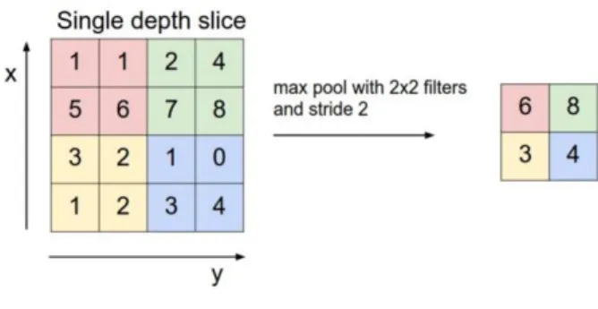
2.2.2.2. Pooling

Assuming that we don’t use zero-padding, we will get a final convolutional output, c which has n - h + 1 numbers. Typically, we want to take the outputs of the CNN and feed it as input to further layers like a Feedforward Neural Network or a RNN. But, all of those need a fixed length input while our CNN output has a length dependent on the length of the sentence n.

(21)

One clever way to fix this problem is to use max-pooling. A key aspect of Convolutional Neural Networks are pooling layers, typically applied after the convolutional layers. Pooling layers subsample their input. The most common way to do pooling it to apply a max operation to the result of each filter. You don’t necessarily need to pool over the complete matrix, you could also pool over a window. For example, the following shows max pooling for a 2×2 window:

Figure 13: Max pooling

The output of the CNN, c ∊ Rn-h-1_{is the input to the max-pooling layer. The output of the max-pooling} layer is ĉ = max{c}, thus ĉ ∊ R.

The advantage for using pooling is that it reduces the output dimensionality but keeps the most salient information. We can think of each filter as detecting a specific feature, such as detecting if the sentence contains a negation. If the negation phrase occurs somewhere in the sentence, the result of applying the filter to that region will yield a large value, but a small value in other regions. By performing the max pooling, we are keeping information about whether or not the feature appeared in the sentence. But with the downside that we lose information about where exactly that feature appeared.

In general, by applying pooling over the convolutional neural network, we are losing information about features’ locality, but we are keeping the local information of the most important features captured by the filters.

2.2.2.3. Multiple-Filters

Another hyperparameter for the convolutional neural networks is the filter size, defining by how much we want to shift the filter at each step. In all the examples above the filter size was 3, meaning we looked only at a combination of three words each time. We can use multiple filters with different length because each filter will learn to recognize a different kind of word combination.

(22)

2.3. Technical tools and system

2.3.1. Keras

2

Keras is a high-level neural networks API, written in Python and capable of running on top of either TensorFlow, CNTK or Theano. It was developed with a focus on enabling fast experimentation. Being able to go from idea to result with the least possible delay is key to doing good research. It has the following advantages:

● User friendliness: Keras is an API designed for human beings, not machines. It puts user experience front and center.

● Modularity: A model is understood as a sequence or a graph of standalone, fully-configurable modules that can be plugged together with as little restrictions as possible.

● Easy extensibility: New modules are simple to add (as new classes and functions), and existing modules provide ample examples. To be able to easily create new modules allows for total expressiveness, making Keras suitable for advanced research.

● Work with Python: No separate models configuration files in a declarative format. Models are described in Python code, which is compact, easier to debug, and allows for ease of extensibility.

We will use Keras as the technical platform to implement the neural network models discussed in this thesis.

2.3.2. Server

The computation work of this thesis is conducted on a server provided by TALP-UPC3_{. We mainly use} the GPU in that server for computational acceleration. The running environment of the GPU is Cuda version 8.0.44 and cuDNN version 5105.

Following is the hardware information of the GPU device on the server:

Figure 14: Hardware information of the GPU

2_{https://keras.io/}

(23)

Chapter 3.

State of the art

3.1. Character-level convolutional network

In this section, we introduce a character-level convolutional network for word encoding introduced by (Kim et al., 2016).

3.1.1. From word-level to character-level

So far, we have viewed various kind of sequence encoders such as LSTM and CNN. Among those encoders, most of them use word-level embedding, and initialize the weight of the embedding layer with pre-trained word vectors such as GloVe (Pennington et al., 2014). In that way, the words in a sentence are not independent anymore, which helps the encoders to catch more internal information of a sentence. However, it also has its downside. As the growth of vocabulary size in the modern corpus, there will be more and more out-of-vocabulary (OOV) words that are not presented in the pre-trained word embedding vector. As the word-level embedding is blind to subword information (e.g. morphemes), it leads to high perplexities for those OOV words.

Currently, there has been a trend focusing on applying CNNs directly to characters. Character-level models obviate the need for morphological tagging or manual feature engineering, and have the attractive property of being able to generate novel words.

3.1.2. Character-level convolutional network

(Kim et al., 2016) introduces the character-level convolutional networks for the task of language modeling, using the output of the character-level CNN as the input to an LSTM at each time step. The model is evaluated on various languages. Analysis of word representations obtained from the character composition part of the model indicates that the model is able to encode, from characters only, rich semantic and orthographic features.

(24)

Figure 15: Architecture of CharCNN

The main contribution of this model is that the input to the encoder layer at time t is an output from a character-level convolutional neural network (CharCNN), thus the model relies only on character-level inputs. The architecture of the network is shown in figure 15.

Let C be the vocabulary of characters, d be the dimensionality of character embeddings, and Q ∊ R d×|C| be the matrix character embeddings. Suppose that word k ∊ V is made up of a sequence of characters [c1; … ; cl], where l is the length of word k. Then the character-level representation of k is given by the matrix C k_∊_R d×l_{, where the j-th column corresponds to the character embedding for cj (i.e. the cj-th} column of Q).

We apply a narrow convolution between C k_{and a filter (or kernel) H}_∊_R dw_{of width w, after which we} add a bias and apply a nonlinearity to obtain a feature map f k_∊_R i-w+1_.

Specifically, the i-th element of f k_{is given by:}

𝑓𝑘_{[𝑖] = tanh(〈𝐶}𝑘_{[∗, i: i + ω − 1], 𝐻〉 + 𝑏)} ₍₂₆₎

where C k_[_∗_{, i : I + w - 1 ]}_{is the}_{i -}_to_{- (i +w-1) - th}_{column of}_C k_and_〈_{A, B}_〉_{= Tr(AB} T₎_{is the} Frobenius inner product.

Finally, we take the max pooling as the feature corresponding to the filter H (when applied to word k):

𝑦𝑘 _{= max}

𝑖 𝑓 𝑘_[𝑖]

(25)

The idea is to capture the most important feature— the one with the highest value—for a given filter. A filter is essentially picking out a character n-gram, where the size of the n-gram corresponds to the filter width.

Following is an example of the computing for a word ‘absurdity’. Firstly, a convolutional filter matrix H of width w = 3 is initialized.

Figure 16: Initialization of convolutional filter H

After that, the convolutional filter matrix H is applied through the whole word, and result in a word representation vector f.

Figure 17: Convoltional computation

Finally, the max-over-time is applied to the word representation vector f to capture the most important feature, and get the result y.

(26)

We have described the process by which one feature is obtained from one filter matrix. Our CharCNN uses multiple filters of varying widths to obtain the feature vector for k. So if we have a total of h filters

H1, …, Hh, then yk = [y1k, … , yhk ] is the input representation of k. For many NLP applications h is typically chosen to be in [100; 1000].

Figure 19: Multiple convolutional filters

We could simply replace xk_{(the word embedding) with y}k_{at each t in the RNN encoder, and this simple} model performs well on its own. Instead we obtained improvements by running yk_{through a highway} network, recently proposed by (Srivastava et al., 2015). Whereas one layer of an MLP applies an affine transformation followed by a nonlinearity to obtain a new set of features,

𝑧 = 𝑔(𝑊𝑦 + 𝑏) (28)

one layer of a highway network does the following:

z = t ⊙ g(𝑊𝐻y + 𝑏𝐻) + (1 − t) ⊙ y (29)

where g is a nonlinearity, t = σ(WT y + bT) is called the transform gate, and (1 - t) is called the carry gate.

Figure 20: Highway layer

Similar to the memory cells in LSTM networks, highway layers allow for training of deep networks by adaptively carrying some dimensions of the input directly to the output. By construction the dimensions of y and z have to match, and hence WT and WH are square matrices.

The advantage of the character-level convolutional network is that the model is able to exploit the character-level information, which will be computed from the characters of corresponding word. By

(27)

doing so, the model gains the ability to learn rich semantic and orthographic features from the encoding of characters.

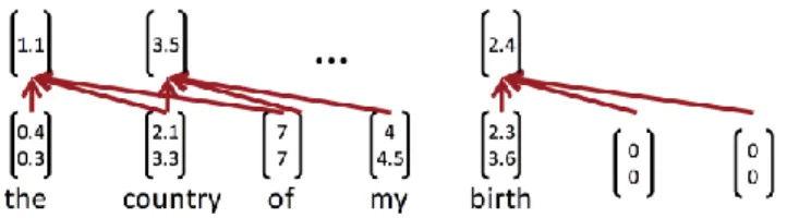
Figure 21 shows the nearest neighbor words learned by CharCNN. The representations of OOV words (computeraided, misinformed) are positioned near words with the same part-of-speech. The model is also able to correct for incorrect/non-standard spelling (looooook), indicating potential applications for text normalization in noisy domains.

Figure 21: The nearest neighbor words learned by CharCNN

3.2. Attention mechanism

In this section, we will discuss the attention mechanism introduced by (Bahdanau et al., 2014). When you hear the sentence "the ball is on the field," you don’t assign the same importance to all 6 words. You primarily take note of the words "ball," "on," and "field," since those are the words that are most "important" to you. Similarly, (Bahdanau et al., 2014) noticed the flaw in using the final RNN hidden state as the single "context vector" for sequence-to-sequence models: often, different parts of an input have different levels of significance. Moreover, different parts of the output may even consider different parts of the input "important." For example, in translation, the first word of output is usually based on the first few words of the input, but the last word is likely based on the last few words of input. Attention mechanisms make use of this observation by providing the decoder network with a look at the entire input sequence at every decoding step; the decoder can then decide what input words are important at any point in time. There are many types of encoder mechanisms, but we’ll examine the one introduced by (Bahdanau et al., 2014).

(28)

Figure 22: Attention mechanism by Bahdanau et al.

The attention mechanism introduced by (Bahdanau et al., 2014) is consisted of two parts, an encoder that encodes the input sentence, and a decoder that leverages the information to produce the translated sentence. Basically, our input is a sequence of words x1, … , xn that we want to translate, and our target sentence is a sequence of words y1, … , ym.

Firstly, let’s take a look at the encoder part. Let (h1, … , hn) be the hidden vectors representing the input sentence. These vectors are the output of a RNN based encoder such as LSTM, that capture contextual representation of each word in the sentence.

Secondly, those vectors will be passed to the decoder to form a new sequence in another language. We compute the hidden states si of the decoder using a recursive formula of the form:

𝑠𝑖= 𝑓(𝑠𝑖−1, 𝑦𝑖−1, 𝑐𝑖) (30)

where si-1 is the previous hidden vector, yi-1 is the generated word at the previous step, and ci is a context vector that capture the context from the original sentence that is relevant to the time step i of the decoder. The context vector ci captures relevant information for the i-th decoding time step. For each hidden vector from the original sentence hj, compute a score:

𝑒𝑖= 𝛼(𝑠𝑖−1, ℎ𝑖) (31)

where α is any function with values in R, for instance a single layer fully-connected neural network. Then, we end up with a sequence of scalar values ei,1, … , ei,n. Normalize these scores into a vector αi =

(αi,1, … , αi,n), using a softmax layer:

𝛼_𝑖𝑗

=

_{∑ exp⁡(𝑒}exp⁡(𝑒𝑖𝑗) 𝑖𝑘)

𝑘 (32)

Then, compute the context vector ci as the weighted average of the hidden vectors from the original sentence:

𝑐𝑖

= ∑

𝑛𝑗=1

𝛼

𝑖,𝑗

ℎ

𝑗 (33)

Intuitively, this vector captures the relevant contextual information from the original sentence for the i-th step of the decoder.

(29)

The attention-based model learns to assign significance to different parts of the input for each step of the output. In the context of translation, attention can be thought of as "alignment." Noting this, we can use attention scores to build an alignment table – a table mapping words in the source to corresponding words in the target sentence – based on the learned encoder and decoder from our system, as shown in figure 23.

Figure 23: Visualization of attention weights

The major advantage of attention-based models is their ability to efficiently encode long sentences. As the size of the input grows, models that do not use attention will miss information and precision if they only use the final representation. Attention is a clever way to fix this issue and experiments indeed confirm the intuition.

This kind of attention between RNNs has a number of other applications. One popular use of this kind of attention is for image captioning. First, a convolutional network processes the image, extracting high-level features. Then an RNN encoder is implemented upon the output of the CNN layer, to generate a sentence description of the image. As it generates the description, the attention will focus on different part of the image for relevant words. We can explicitly visualize this in figure 24.

Figure 24: Attention mechanism for image

More broadly, attentional mechanism can be used whenever one wants to align some feature with the RNN encoders. Attentional mechanism have been found to be an extremely general and powerful technique, and are becoming increasingly widespread.

(30)

Chapter 4.

Development of the Model

4.1. Baseline Model

In this section, the baseline model introduced by (Adina Williams et al., 2017) will be discussed. The baseline model is a 5-layer architecture model, which can be seen as in figure 25. It has two inputs, premise input and hypothesis input. The model first encodes the sentence input into a fixed length vector. Then it use the encoded vectors to determine the directional relationship between premise input and hypothesis input.

Figure 25: Baseline model architecture

The first layer in the bottom is the input layer, which is consisted of a sequence of words. The length of the sequence is defined as 50 here, and the words are tokenized to real numbers.

The second layer is the word embedding layer. It transforms each input text sentence into a vector, with a fixed dimension [50, 300]. The first dimension is the length of a sentence, which means the number of words in a sentence. Here we choose 50 as the length of a sentence. If the sentence length is longer than 50, it will be truncated. If the sentence length is shorter than 50, it will be padded to 50 using zero vector. The second dimension means the dimension of a single word. Here we use 300-dimension vector to represent the meaning of each word. It will be randomly initialized and updated during the training period.

The third layer is the sentence encoder layer. It transforms each sentence with word embeddings into a single embedding vector, with a fixed dimension (300). Here we use the LSTM encoder introduced in

(31)

Chapter 2. It will encode the sentence word by word, and concatenate the sequence into a single vector, which represent the meaning of the sentence.

Since the premise and hypothesis texts have similar structure, so we use shared weights for the first layer and second layer. It can make these layers more robust and also shorten the training time reaching model convergence.

The fourth layer is the concatenation of the premise encoded vector and the hypothesis encoded vector. It then passes the concatenated vector though 3 MLP layers (densely connected layer) with RELU as the activation function.

The fifth layer, which is our last layer, is a MLP layer with the softmax activation function. It has an output of dimension (3), so it’s also called a 3-way softmax layer. The result reflects the directional relationship between the premise input sentence and the hypothesis input sentence.

4.2. Character-level Intra Attention Networks

In this section, we will augment the baseline model, so that it can perform better on the textual entailment task. Two main improvements have been implemented based on the baseline model. One is the character-level convolutional network, another is the intra-sentence attention mechanism. Those two augments will be introduced and explained in detail in the following paragraph.

In the baseline BiLSTM model, the input xt to the encoder layer at time t are pre-trained word embeddings. Those pre-trained word embeddings can boost the performance of the model. However, it is limited to the finite-size of the pre-trained embedding vocabulary. Here we take place of the word embedding layer with a character-level convolutional network (CharCNN) introduced by (Kim et al., 2016) for language modeling.

We define a sentence representation vector as 𝐶𝑘_{∈ ℝ}𝑑×𝑙_{, where}_d_{is the dimensionality of character} embeddings,𝑙 is the length of 𝑘-th word in a sentence. Then a set of narrow convolutions between 𝐶𝑘 and filter 𝐻 is applied, followed with a max-over-time (max pooling) as shown in formula (34-35).

𝑓𝑘_{[𝑖] = tanh(〈𝐶}𝑘_{[∗, i: i + ω − 1], 𝐻〉 + 𝑏)} 𝑦𝑘 _{= max} 𝑖 𝑓 𝑘_[𝑖] (34) (35) The concatenation of those max values provides us with a representation y𝑘_{of each word}_k_{as a vector of} convolutional kernels.

Then, a highway network is applied upon y𝑘_{, as shown in formula (36).}

z = t ⊙ g(𝑊𝐻y + 𝑏𝐻) + (1 − t) ⊙ y (36)

where g is a nonlinearity, t = σ(𝑊𝑇y + 𝑏𝑇) is called the transform gate, and (1 − t) is called the carry gate. Highway layers allow for training of deep networks by adaptively carrying some dimensions of

(32)

After it, the sequence of encoded words will be passed to the BiLSTM encoder introduced in section 2.2.1. We use 300D hidden states in the encoder, thus 600D hidden states as it’s bidirectional.

In the baseline BiLSTM model, the sentence representation h as the output of LSTM is an average pooling over the LSTM hidden states [h0, h1, … , h𝑛]. However, this has its bottleneck as we intuitively know that not all words contribute equally to the sentence representation. To augment the performance of RNN based encoder, the concept of Intra Attention mechanism introduced by (Z. Yang et al., 2016) is implemented here. We define the hidden states of the RNN based encoder as ℎ𝑡∈ [h0, h1, … , h𝑛], the intra attention is applied upon the hidden states to get the sentence representation vector, specifically,

𝑢𝑡= tanh(𝑊𝜔ℎ𝑡+ 𝑏𝜔) 𝛼_𝑡

=

exp⁡(𝑢

𝑡 𝑇

_𝑢

𝜔

)

∑ exp⁡(𝑢

_𝑡𝑇

_𝑢

𝜔

)

𝑡 s = ∑ 𝛼𝑡ℎ𝑡 𝑡 (37) (38) (39) It first feed the hidden states ℎ𝑡 through a one-layer MLP to get 𝑢𝑡 as the hidden representation of ℎ𝑡. Then it uses a softmax function to catch the normalized importance weight matrix 𝑎𝑡. After that, the sentence representation vector s is computed by a weighted sum of all hidden states ℎ𝑡 with the weight matrix 𝑎𝑡. The context vector u𝜔 can be seen as a high-level representation of the importance of the informative word over the words in memory networks (Sukhbaatar et al., 2015; Kumar et al., 2015). The computational cost of this attention step is constant and does not explode with the length of the sentence. The final model is shown as follows. It consists of 7 layers, of which the first layer and the last two layers are the same with our baseline model. The 4 layers in middle are our augmented layers that we’ve introduced in detailed in this chapter.

Figure 26: CIAN model architecture

(33)

Layer Output Shape Number of Parameters

Input layer (50, 15) 0

CNN layer with Maxpooling (50, 1100) 83035

Highway layer (50, 1100) 4844400

BiLSTM layer (50, 600) 3362400

Intra Attention layer (600) 186000

ReLU layer (300) 1449000

3-way Softmax layer (3) 1803

Total parameters: 9,931,038

Table 3: Detail information for CIAN model

4.3. Tricks in practice

In this section, we will discuss some practical tricks when training the neural network.

4.3.1. Dropout

Dropout is a powerful technique for regularization, first introduced by (Srivastava et al, 2015). The idea is simple yet effective – during training, we will randomly “drop” with some probability (1 - p) a subset of neurons during each forward/backward pass (or equivalently, we will keep alive each neuron with a probability p). Then, during testing, we will use the full network to compute our predictions. The result is that the network typically learns more meaningful information from the data, is less likely to overfit, and usually obtains higher performance overall on the task at hand. One intuitive reason why this technique should be so effective is that what dropout is doing is essentially doing is training exponentially many smaller networks at once and averaging over their predictions.

(34)

4.3.2. Normalization

Another frequently used trick is to scale every input feature dimension to have similar ranges of magnitudes. This is useful since input features are often measured in different “units”, but we often want to initially consider all features as equally important. The way we accomplish this is by simply dividing the features by their respective standard deviation calculated across the training set.

(35)

Chapter 5.

Evaluation of the model

5.1. Evaluation method

We evaluate our approach on the Multi-Genre NLI (MNLI) corpus (Adina Williams et al., 2017), as a shared task for RepEval4_{2017 workshop. The task here is to do the textual entailment as a three-way} classification task. Given a sentence pair (a, b), the task is to predict whether b is entailed by a, b is contradicted to a, or whether the relation between a and b is neutral.

We train our model on a mixture of MNLI and SNLI corpus, by using a full MNLI training set and a randomly selected 20% of the SNLI training set at each epoch.

The evaluation includes two test datasets, a standard in-domain (matched) evaluation in which the training and test data are drawn from the same sources, and a cross-domain (mismatched) evaluation in which the training and test data differ substantially.

5.2. Result and analysis

The CIAN model is implemented5_{as described in Chapter 3. The characters tokenization list in the CNN} layer are [abcdefghijklmnopqrstuvwxyz012 3456789-,;.!?:'"/\|_@#$%^&*~`+-=<>()[]{}]. The input text will firstly be set to lowercase, then it will be vectorized according to the tokenization list. Those characters not in the list will be initialized with a vector of 0. We use 7 filters in CIAN model’s CNN layer.

The widths of the filters are w = [1, 2, 3, 4, 5, 6, 7] , and the corresponding filters’ size are [min{200, 50 ∙ 𝑤}]. Two highway layers are implemented following the CNN layer. The attention layer uses the hidden states of the BiLSTM encoder to encode each sentence into a fixed-length single vector. Dropout (Srivastava et al., 2014) is implemented with a dropout rate of 0.2 to prevent the model from overfitting. The Adam optimizer (Kingma et al., 2014) is used for training with backpropagation.

4_{https://repeval2017.github.io/}

(36)

The model is implemented using Keras, the training takes approximately one hour for one epoch on GeForce GTX TITAN.

The training and validation accuracy is shown in the following figure. It can be seen that the training accuracy keeps increasing until 80%, while the validation accuracy rises to 68% in 20-th epoch and nearly stops increasing after that. We stopped the training on the 28-th epoch as the validation accuracy stops increasing, which is also a way to prevent from overfitting.

Figure 28: Training and validation accuracy during training

The following table shows the test accuracy for the baseline model and the CIAN model upon matched and mismatched test dataset. The accuracy of the baseline model is improved with 0.9 percent in matched test set, and 0.6 percent in mismatched test set.

Model Matched Mismatched

BiLSTM 67.0 67.6

CIAN 67.9 68.2

Table 4: Experiment results

Our CIAN model outperforms the baseline model, and it also success in the mismatched test dataset. This cross-domain evaluation on the mismatched dataset shows the ability of our model to learn representations of sentence meaning that capture broadly useful features.

We also conduct error analysis based on expert-tagged development data released by the organizers of RepEval 2017 shared task. The tags are defined below.

(37)

Tag Definition

CONDITIONAL Whether any sentence in the pair contains a conditional Example: (mismatched-362738n)

laser-cutting equipment must be totally enclosed to be safe for human operators.

even if the laser machine is fully contained within, there still exist some amount of risk for the workers in the close proximity.

ACTIVE/PASSIVE Whether there is an active to passive (or vice versa) transformation between the premise and the hypothesis

Example: (mismatched-59050c)

hani hanjour, khalid al mihdhar, and majed moqed were flagged by capps

capps never flagged anyone.

PARAPHRASE Whether the premise and the hypothesis are paraphrases Example: (mismatched-177012e)

uh, lets see let us look.

COREF Whether the hypothesis contains a pronoun or referring expression that need to be resolved using the premise.

Example: (mismatched-297191e)

*you and i, gentle reader,* are accredited members of the guild. *we* are recognised as members of the guild.

QUANTIFIER Whether premise or hypothesis contain one of the quantifier from the QUANTIFIER list

we have provided an invoice to facilitate your gift. there's no invoice available for your gift.

MODAL Whether premise or hypothesis contain one of the model verbs from the MODAL_VERBS list

i trust that this is a fillip of propaganda and not a serious query. i believe this is to get attention and not a real inquiry.

BELIEF Whether premise or hypothesis contain one of the model verbs from the BELIEF_VERBS list

i trust that this is a fillip of propaganda and not a serious query. i believe this is to get attention and not a real inquiry.

NEGATION Whether premise or hypothesis contain a negation Example: (mismatched-148280c)

(38)

ANTO Whether premise and hypothesis contain antonyms Example: (mismatched-59395c)

as united 93 left newark, the flight's crew members were *unaware* of the hijacking of american 11.

as the flight united 93 left newark the crew members were fully *aware* of the hijacking of american 11.

TENSE_DIFFERENCE Whether premise and hypothesis are expressed in difference tenses Example: (mismatched-176769e)

does she like what she *does*? does she like what she *is* doing*? QUANTITY/

TIME_REASONING

Whether the hypothesis needs quantity or time reasoning

Example: - time_reasoning (mismatched-59568c)

the vice chairman joined the conference shortly before *10:00*; the secretary, shortly before *10:30*.

the secretary joined *before* the vice chairman. - quantity_reasoning

(mismatched-58841c)

the call lasted about *two minutes*, after which policastro and a colleague tried unsuccessfully to contact the flight.

the call only lasted *5 seconds* before it was dropped. WORD_OVERLAP Whether hypothesis and premise overlap more than 70%.

Example: (mismatched-62885c) let's look for paua shells! let's look for sticks.

LONG_SENTENCE Whether premise or hypothesis are longer than 30 or 16 words respectively.

as invested with its dignity, since the seventeenth century just as the crown has been used for the monarch, or the oval office has come to stand for the president of the united states.

nobody in britain associates the crown with the monarchy.

Table 5: Definition of the development tags

The results for error analysis are shown in Table 6. From the results, it can be seen that the accuracy for WORD_OVERLAP, LONG_SENTENCE, ACTIVE/PASSIVE and PARAPHRASE have been improved significantly in both matched and mismatched development set. Which clarifies the ability of character-level convolutional network for encoding words with the semantic and orthographic meaning, and the ability for intra attention layer to encode long sentences. While the accuracy for CONDITIONAL and COREF have been decreased in both development set.

(39)

Matched Mismatched

Tag BiLSTM CIAN BiLSTM CIAN

CONDITIONAL 100 48 100 62 WORD_OVERLAP 50 79 57 62 NEGATION 71 71 69 70 ANTO 67 82 58 70 LONG_SENTENCE 50 68 55 63 TENCE_DIFFERNCE 64 65 71 72 ACTIVE/PASSIVE 75 87 82 90 PARAPHRASE 78 88 81 89 QUANTITY/TIME_REASONING 50 47 46 44 COREF 84 67 80 72 QUANTIFIER 64 63 70 69 MODAL 66 66 64 70 BELIEF 74 71 73 70

Table 6: Accuracy for expert-tagged development data

5.3. Visualization

A nice advantage of implementing attention mechanism in the model is that we can visualize the attention weights. By doing so, we can enhance the interpretability of the model and understand how it judges the textual entailment relation between two sentences.

Following are visualizations for 6 sentence pairs, with the premise at top and hypothesis at below. As a balance, 2 pairs are with entailment relation, 2 pairs with neural and 2 pairs with contradiction. The pairID and their relation will be tagged in the name of the figures.

(40)

(41)

(42)

(43)

(44)

(45)

(46)

Chapter 6.

Conclusion

In this paper, we presented a Character-level Intra Attention Networks (CIAN) for the task of natural language inference. Experimental results demonstrate that our model outperforms the baseline model upon the MultiNLI corpus.

To summarize, the CIAN model presented in this paper is a sequence encoder that has the ability to to encode long sentence in character-level with rich semantic and orthographic features. Also, the attention mechanism provides high interpretability of the model that allows people to understand how the model doing its task. As it’s an end-to-end neural network that does not need any specific pre-processing or outside data like pre-trained word embeddings. It can be easily applied to other encoder architecture tasks such as language modeling, sentiment analysis and question answering.

It can be foreseen that deep learning will come to dominate the NLP field over the next couple of years. This is a good thing as deep learning provides a way to solve problems that are easy for people to perform but hard for people to describe formally. With the power of deep learning we can have our computer more intelligent to deal with the hard tasks couldn’t be solved before. However, we should also realize that there is currently a overconfidence about deep learning and artificial intelligence. Deep learning is just part of the machine learning technique that improves its performance with experience and data. We should not let our enthusiasm lead to an irrational craze or a reduction on other technical approaches.

Recognizing textual entailment using deep learning techniques