A robust experimental evaluation of automated multi-label classification methods

(1)

Kent Academic Repository

Full text document (pdf)

Copyright & reuse

Content in the Kent Academic Repository is made available for research purposes. Unless otherwise stated all

content is protected by copyright and in the absence of an open licence (eg Creative Commons), permissions

for further reuse of content should be sought from the publisher, author or other copyright holder.

Versions of research

The version in the Kent Academic Repository may differ from the final published version.

Users are advised to check

http://kar.kent.ac.uk

for the status of the paper.

Users should always cite the

published version of record.

Enquiries

For any further enquiries regarding the licence status of this document, please contact:

[email protected]

If you believe this document infringes copyright then please contact the KAR admin team with the take-down

information provided at

http://kar.kent.ac.uk/contact.html

Citation for published version

de Sá, Alex G. C. and Pimenta, Cristiano G. and Pappa, Gisele L. and Freitas, Alex A. (2020)

A robust experimental evaluation of automated multi-label classification methods. In: GECCO

'20: Proceedings of the 2020 Genetic and Evolutionary Computation Conference. ACM, New

York, USA, pp. 175-183. ISBN 978-1-4503-7128-5.

DOI

https://doi.org/10.1145/3377930.3390231

Link to record in KAR

https://kar.kent.ac.uk/82232/

Document Version

Author's Accepted Manuscript

(2)

Classification Methods

Alex G. C. de Sá

Computer Science Department Universidade Federal de Minas Gerais

Belo Horizonte, MG, Brazil [email protected]

Cristiano G. Pimenta

Gisele L. Pappa

Alex A. Freitas

School of Computing University of Kent Canterbury, Kent, United Kingdom

[email protected]

ABSTRACT

Automated Machine Learning (AutoML) has emerged to deal with the selection and configuration of algorithms for a given learning task. With the progression of AutoML, several effective methods were introduced, especially for traditional classification and re-gression problems. Apart from the AutoML success, several issues remain open. One issue, in particular, is the lack of ability of Au-toML methods to deal with different types of data. Based on this scenario, this paper approaches AutoML for multi-label classifica-tion (MLC) problems. In MLC, each example can be simultaneously associated to several class labels, unlike the standard classifica-tion task, where an example is associated to just one class label. In this work, we provide a general comparison of five automated multi-label classification methods ś two evolutionary methods, one Bayesian optimization method, one random search and one greedy search ś on 14 datasets and three designed search spaces. Overall, we observe that the most prominent method is the one based on a canonical grammar-based genetic programming (GGP) search method, namely Auto-MEKA𝐺𝐺𝑃. Auto-MEKA𝐺𝐺𝑃presented the

best average results in our comparison and was statistically better than all the other methods in different search spaces and evaluated measures, except when compared to the greedy search method.

CCS CONCEPTS

·Computing methodologies→Machine learning approaches;

Machine learning;Search methodologies;Genetic programming;

Randomized search;

KEYWORDS

Automated Machine Learning (AutoML), Multi-Label Classification, Search Methods, Search Spaces

Permission to make digital or hard copies of all or part of this work for personal or classroom use is granted without fee provided that copies are not made or distributed for profit or commercial advantage and that copies bear this notice and the full citation on the first page. Copyrights for components of this work owned by others than ACM must be honored. Abstracting with credit is permitted. To copy otherwise, or republish, to post on servers or to redistribute to lists, requires prior specific permission and/or a fee. Request permissions from [email protected].

ACM Reference Format:

Alex G. C. de Sá, Cristiano G. Pimenta, Gisele L. Pappa, and Alex A. Freitas. 2020. A Robust Experimental Evaluation of Automated Multi-Label Clas-sification Methods. InGenetic and Evolutionary Computation Conference (GECCO ’20), July 8ś12, 2020, Cancún, Mexico.ACM, New York, NY, USA, 9 pages. https://doi.org/10.1145/3377930.3390231

1 INTRODUCTION

We are experiencing the era of data. With its great availability, people in general (e.g., practitioners, data scientists, and researchers) are trying hard to extract useful information encoded on data [22]. This resulted in an ever-growing popularity and the indiscriminate use of machine learning (ML) algorithms by many types of users.

The field ofAutomated Machine Learning(AutoML) [13] has emerged to help this wide and heterogeneous public. This field has the purpose of democratizing ML in a way ML can be used with less difficulties by general audiences. In addition, AutoML also aims to assist experienced data scientists. In both scenarios, the field of AutoML has the scope of recommending learning al-gorithms (and often their hyper-parameters’ settings too) when people face a particular problem that might be (partially or totally) solved with ML. Broadly speaking, AutoML proposes to deal with users’ biases by customizing the solutions (in terms of algorithms and configurations) to ML problems following different approaches. AutoML has been successfully and mainly employed to solve traditional (single-label) classification and regression problems [9]. However, this work is interested in AutoML methods for a different and specific type of data, calledMulti-Label Classification(MLC) [11, 26, 30]. The goal of MLC is to learn a model that expresses the rela-tionships between a set of predictive features (attributes) describing the examples and a predefined set of class labels. In MLC, each ex-ample can be simultaneously associated to one or more class labels. Each class label is represented by a discrete value.

When compared to single-label classification (SLC), MLC can be considered a more challenging task, mainly due to the following reasons. First, an MLC algorithm needs to consider the label corre-lations (i.e., detecting whether or not they exist) in order to learn a model that produces accurate classification results [30]. Second, given the usual limited number of examples for each class label in the dataset [11], the generalization in MLC is considered harder than SLC, as the MLC algorithm needs more examples to create a good model from such complex data [7]. Third, there is a strain

(3)

GECCO ’20, July 8–12, 2020, Cancún, Mexico

to evaluate MLC classifiers as several metrics follow contrasting aspects to define what is a good MLC prediction [18]. Finally, the learning algorithms applied to solve MLC problems need more computational resources than the ones used to solve SLC [11]. This is mainly due to MLC being a generalization of SLC, so that the algorithms need to look at several labels instead of just one.

We claim that these aforementioned challenges are part of the reason why AutoML for MLC problems (i.e., AutoMLC) has not been sufficiently explored. Taking it into consideration, this work performs an assessment of popularsearch methodsfor AutoMLC, including evolutionary methods, a Bayesian optimization method and blind-search methods. For that, we propose two novel AutoMLC

search methods. The first is an extension of the work of de Sáet

al.[4] on Grammar-based Genetic Programming (GGP) [16, 28] for AutoMLC, named Auto-MEKA𝐺𝐺𝑃. Our extension adds to the GGP

core a speciation approach [1] aiming to improve the diversity of the produced solutions. The secondsearch methodis a Bayesian optimization (BO) method, namely Sequential Model-based Algo-rithm Configuration (SMAC) [12] ś note that there was no such methods previously proposed in the AutoMLC literature. As both proposed methods are based on the well-known MLC MEKA frame-work [20], we named thesesearch methodsas Auto-MEKA𝑠𝑝𝐺𝐺𝑃

and Auto-MEKA𝐵𝑂, respectively.

We compare these two proposedsearch methodswith Auto-MEKA𝐺𝐺𝑃[4], a random search (namely, Auto-MEKA𝑅𝑆) and a

greedy search (namely, Auto-MEKA𝐺𝑆) on three designed MLC

search spaces (namely, Small, Medium and Large) over 14 bench-marking datasets. Finally, in this work, we use five performance measures for evaluating these methods, due to the additional degree of freedom that the MLC algorithms’ setting introduces [14].

The experimental results show that Auto-MEKA𝐺𝐺𝑃mostly

pre-sented the best average results and also the best average ranks for severalsearch spacesand measures. Besides, Auto-MEKA𝐺𝐺𝑃was

the only method to be statistically better than all other evaluated

search methodsin different occasions (i.e., performance measures

versus search spaces), except when compared to Auto-MEKA𝐺𝑆.

Although this is a positive result for the evolutionary methods, we believe that more robust methods ś such as Auto-MEKA𝐺𝐺𝑃,

Auto-MEKA𝑠𝑝𝐺𝐺𝑃 and Auto-MEKA𝐵𝑂ś can still improve their

predictive performances. With this in mind, we observe that these methods could not satisfactorily trade-off between exploration and exploitation as they were not statistically and simultaneously better than pure-exploration and pure-exploitation methods (i.e., Auto-MEKA𝑅𝑆and Auto-MEKA𝐺𝑆, respectively).

The results also show that there is a high correlation between the size (and definition) of the search space and the effectiveness of AutoMLC methods to select and configure algorithms. When looking at the predictive accuracy of the AutoMLC methods, we have an indication that as the size of an AutoMLC’ssearch space

decreases, pure-exploration and/or pure-exploitation AutoMLC

search methodstend to have similar results to robust AutoMLC

methods (such as the ones presented in this work).

The remainder of this paper is organized as follows. Section 2 introduces MLC and Section 3 reviews related work on AutoMLC. Section 4 details AutoMLC in terms of the proposedsearch spaces

and evaluatedsearch methodsthat are included in the experimental comparison, while Section 5 presents and discusses the obtained

results. Finally, Section 6 draws some conclusions and discusses directions for future work.

2 MULTI-LABEL CLASSIFICATION

There is a great number of works on traditional single-label classifi-cation (SLC) for machine learning (ML) [29]. In SLC, each example is defined by a tuple (𝑋 , 𝑦), where𝑋 ={𝑥1, ..., 𝑥𝑑}is a𝑑-dimensional

vector representing the feature space (i.e., the categorical and/or numerical characteristics of that example) and𝑦is the class value, where𝑦∈𝐿, a set of disjoint class labels. In SLC, each example is strictly associated to a single class label.

Nevertheless, there is an increasing number of applications that require associating an example to more than one class label [10], such as medical diagnosis and protein function prediction. This classification scenario is better known asMulti-Label Classifica-tion(MLC). According to [25], each example in MLC is represented by a tuple (𝑋,𝑌), where𝑋is the𝑑−dimensional feature vector, and

𝑌 ⊆𝐿is a set of non-disjoint class labels. Hence, we would like to find an MLC modelℎ:𝑋 →2|𝐿|such thatℎmaximizes a quality criterion𝜆.

The literature divides MLC algorithms into three categories [10]: problem transformation (PT), algorithm adaptation (AA) and ensem-ble or meta-algorithms methods (Meta-MLC). Whereas PT methods transform the multi-label problem into one or more single-label classification problems, AA methods simply extend single-label classification algorithms so they can directly handle multi-label data. Finally, Meta-MLC methods act on top of PT or AA multi-label classifiers, aiming to combine the results of MLC algorithms and produce models with more robust predictive performances.

Among the great number of MLC algorithms [11, 26, 30], it is important to mention three methods that transform an MLC prob-lem into one or many SLC probprob-lems: Label Powerset (LP), Binary Relevance (BR) and Classifier Chain (CC). LP creates a single class for each unique set of labels that is associated with at least one example in a multi-label training set. BR, in turn, learns|𝐿| indepen-dent binary classifiers, one for each label in the labelset𝐿. Finally, CC changes the BR method by chaining the binary classifiers. In this case, the feature space of each link in the chain is increased with the classification outputs of all previous links.

3 RELATED WORK ON AUTOMLC

Most AutoML methods in the literature were designed to solve the conventional single-label classification and regression tasks [9], and can not handle multi-label data. As far as we know, there are only a few works related toAutomated Multi-Label Classification (Au-toMLC).

[3] developed a meta-model (i.e., a 20-Nearest Neighbors clas-sifier) for selecting one out of 11 multi-label classification algo-rithms, taking into account 30 characterizing measures and 36 meta-datasets. Nevertheless, as it is a preliminary work, it only selects the MLC algorithm, not setting the algorithm’s hyper-parameters. Evolutionary Multi-Label Ensemble (EME) [17] encompasses the problem of selecting MLC algorithms to compose MLC ensembles. The main idea of EME stands on the simplicity of each ensemble’s multi-label classifier, which is focused on a small subset of the labels, but still considering the relationships among them and avoiding the high complexity of the output space. Nevertheless, EME takes into account only one type of model to compose the ensembles (i.e.,

(4)

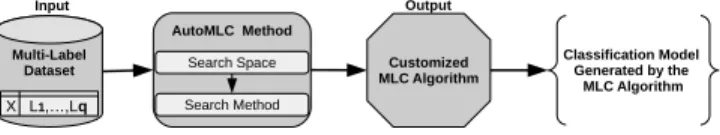
Multi-Label Dataset AutoMLC Method Output Input Customized MLC Algorithm X L1,…,Lq Search Method

Search Space Classification Model _{Generated by the}

MLC Algorithm

Figure 1: The general AutoMLC framework to select and con-figure MLC algorithms.

the model produced by label powerset), so it is not sufficient to deal with all types of MLC problems.

Furthermore, [27] proposed an extension to a canonical hierar-chical planing method (i.e., ML-Plan) to the MLC context. They named this method as ML2-Plan (Multi-Label ML-Plan). Basically, ML2-Plan is implemented as a global best-first search over the graph induced by the planning problem at hand.

Finally, [4, 5] proposed two AutoML methods for MLC prob-lems: GA-Auto-MLC and Auto-MEKA𝐺𝐺𝑃. Whereas GA-Auto-MLC

employs a real-coded genetic algorithm [8] to perform its search, Auto-MEKA𝐺𝐺𝑃uses a grammar-based genetic programming

al-gorithm [16, 28]. Auto-MEKA𝐺𝐺𝑃is a robust enhancement of

GA-Auto-MLC to handle huge and, consequently, complex MLCsearch

spaces. Because of that, we decided to only include Auto-MEKA𝐺𝐺𝑃

into our experiments. We will further discuss it in Section 4.

4 AUTOML METHODS FOR MULTI-LABEL

CLASSIFICATION

This section introduces a generic AutoMLC framework followed by all AutoMLC methods evaluated in this paper. As illustrated in Figure 1, the AutoMLC method receives as input a specific multi-label dataset (with the feature space𝑋 and the class labels𝐿1to

𝐿𝑞). Structurally, the evaluated AutoMLC methods have two main

components: thesearch spaceand thesearch method.

Thesearch spaceconsists of the main building blocks (e.g., the

prediction threshold values, the hyper-parameters and the algo-rithms at the SLC level) from previously designed MLC algoalgo-rithms. To explore thissearch space, the AutoMLC method uses asearch

method, which finds appropriate MLC algorithms to the dataset at

hand. However, the performance of thesearch methoddepends on what is specified in thesearch space.

Once the search is over, the AutoMLC method outputs an MLC al-gorithm tailored to the input dataset based on thatsearch space. This MLC algorithm is specifically selected and (hyper-)parameterized to this dataset, although it could be applied to any multi-label dataset. In the end, the customized MLC algorithm returns an MLC model, and consequently, its classification results.

The evaluation presented in this paper considers threesearch

spaces, namely Small, Medium and Large, which differ from each

other in terms of complexity. These threesearch spacesare explored using fivesearch methods: Auto-MEKA𝐺𝐺𝑃, Auto-MEKA𝑆𝑝𝐺𝐺𝑃,

Auto-MEKA𝐵𝑂, Auto-MEKA𝑅𝑆and Auto-MEKA𝐺𝑆, as detailed in

Section 4.2.

4.1 Search Spaces

To design thesearch spacesfor the AutoMLC methods being evalu-ated, we first performed a deep study about multi-label classification in the MEKA software. We analyzed in detail all the algorithms and their hyper-parameters, the constraints associated with different

hyparameter settings, the hierarchical nature of operations per-formed by problem transformation methods and meta-algorithms, among other issues.

Based on that, we designed threesearch spaces1: Small, Medium and Large. The reason behind this threefold modeling is basically because we want to test different levels ofsearch spacecomplexity. For thesearch spaceSmall, for instance, we have five MLC al-gorithms, where four of them can be combined with other five SLC algorithms, as they are from the PT category. The only algo-rithm that can not be combined with SLC algoalgo-rithms is ML-BPNN, which belongs to the AA category. Therefore, thesearch spaceSmall consists of 10 learning algorithms ś five MLC algorithms and five SLC algorithms, which gives a set of 21 combinations of learning algorithms, where the AA category counts as one combination.

In contrast, thesearch spaceMedium has 30 learning algorithms ś 15 MLC algorithms and 15 SLC algorithms, which produces 211 combinations of algorithms. Finally, thesearch spaceLarge has a total of 54 learning algorithms ś 26 MLC algorithms and 28 SLC al-gorithms, which produces 16,568 possible combinations of learning algorithms.

Although the main difference between the Small and Medium

search spacesis the number of learning algorithms, note that, when

comparing Medium to Large, we have a change on the structure of thesearch space. This happens because we only added meta-algorithms at the MLC and SLC levels into Large. Hence, we have more levels in the multi-label hierarchy to consider. For example, when asearch methodis selecting a new MLC algorithm in this

search space, it must decide whether to include or exclude

meta-algorithms at the MLC and SLC levels. As a result, thissearch space

is hierarchically more complex than the other two (i.e., Small and Medium).

Taking into account the number of learning algorithms, the number of hyper-parameters, and the constraints in the choices of algorithms’ components and (hyper)-parameters in MEKA, we estimated the size of the threesearch spaces2. In total, thesearch spaceSmall has[(5.070×107) + (8.078×108×𝑚) + (2.535×1010×𝑞)]

possible MLC algorithm configurations (i.e., a given set of learning algorithms with their respective hyper-parameters), where𝑚is the number of features (or attributes) and𝑞is the number of labels of the dataset. Thesearch spaceMedium, on the other hand, is estimated as having[(2.545×1016) + (8.078×108×𝑚) + (1.151×1012×𝑞)]

possible MLC algorithm configurations. Finally, thesearch space

Large is estimated to have approximately[(6.555×1029) + (1.443×

1014_×𝑚) + (3.042_×1022_×𝑞) + (1.291_×1027_×√𝑞)]possible MLC algorithm configurations.

4.2 Search Methods

This section details the fivesearch methodsused in our comparison. They all follow the same methodology.

Eachsearch methodstarts its own iterative process by

gener-ating, evaluating and looking for MLC algorithms configurations. To perform the evaluation, thesearch methodsuse the average of four well-known measures [10, 25]: Exact Match (EM), Hamming Loss (HL),𝐹1Macro averaged by label (FM) and Ranking Loss (RL),

1_{For more details about the MLC and SLC algorithms and meta-algorithms that}

com-pose thesearch spaces, see the supplementary material.

2_{In these estimations, the real-valued hyper-parameters have always taken 100 different}

(5)

as indicated in Equation 1. Thesearch methodkeeps iterating while a maximum time budget is not reached. At the end, the best MLC algorithm configuration in accordance to the quality criteria is returned and assessed in the test set.

𝐹𝑖𝑡𝑛𝑒𝑠𝑠= 𝐸𝑀+ (

1₋𝐻 𝐿) +𝐹 𝑀+ (1₋𝑅𝐿)

4 (1)

Regarding the MLC evaluation measures, EM is a very strict metric, as it only takes the value one when the predicted label set is an exact match to the true label set for an example, and takes the value zero otherwise. HL, in turn, calculates how many example-label pairs are misclassified. Furthermore, FM is the har-monic mean between precision and recall, and its average is first calculated for each label and, after that, across all the labels. Finally, RL measures the number of times that irrelevant labels are ranked higher than relevant labels, i.e., it penalizes the label pairs that are reversely ordered in the ranking for a given example. All four metrics are within the[0,1]interval. However, whereas the EM and FM measures should be maximized, the HL and RL measures should be minimized. Hence, HL and RL are subtracted from one in Equation 1 to make the search maximize the fitness function.

4.2.1 Auto-MEKAGGP.This method was proposed in [4], and

re-lies on a Grammar-based Genetic Programming (GGP) approach [16, 28], which has the advantage of hierarchically exploring the nature of the AutoMLC problem. In this case, the grammar encompasses

thesearch spaceof MLC algorithms and hyper-parameter settings.

In Auto-MEKAGGP, each individual expresses an MLC algorithm

configuration, and is represented by a derivation tree generated from the grammar. Individuals are first generated by choosing at random a valid production rule, and then mapping it into an MLC algorithm (with a specific hyper-parameter setting).

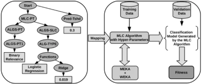
Figure 2 details the whole mapping process followed by the evaluation process for each GGP individual. In the example of Figure 2, ellipsoid nodes are the grammar’s non-terminals, whereas the rectangles are the terminals.

Fitness Validation Data MLC Algorithm with Hyper-Parameters MEKA + WEKA Classification Model Generated by the MLC Algorithm Start MLC-PT Pred-Tshd 0.3 ALGS-SLC ALGS-PT ALG-TYPE Functions Logistic Regression ALGS-PT1 0.019 Binary Relevance Mapping Ridge Training Data

Figure 2: Individual’s evaluation process in Auto-MEKA𝐺𝐺𝑃.

The mapping process takes the terminals from the tree and con-structs a valid MLC algorithm. The mapping in Figure 2 will produce the following MLC algorithm: a Binary Relevance method combined with a Logistic Regression algorithm (with the hyper-parameter ridge set to 0.019), using a threshold of 0.3 to classify the MLC data. Next, individuals have their fitness calculated as previously ex-plained, and undergo tournament selection. The GGP operators (i.e., Whigham’s crossover and mutation [28]) are applied to the selected individuals to create a new population. These operators

also respect the grammar constraints, ensuring that the produced individuals represent valid solutions.

4.2.2 Auto-MEKAspGGP. This novel AutoMLC method enhances

the search mechanisms of Auto-MEKA𝐺𝐺𝑃 by adding a

specia-tion process [1] into itssearch method. The general idea is to use Grammar-based Genetic Programming with Speciation (spGGP) to improve the trade-off between exploration and exploitation of the search for MLC algorithms and hyper-parameter settings. Be-cause the proposedsearch spaceshave an exponential size and a complex hierarchical nature, it may be crucial to use this approach to deal with these aspects. A species is a set of individuals that resemble each other more inherently than the individuals in an-other species [1]. In speciation-based evolutionary computation, the objective is to emphatically restrict mating to those among like individuals from the population. In this case, likeness among indi-viduals is identified if they have similar genotypes or phenotypes. In this work, we defined a set of species based on the types of MLC hyper-parameters (i.e., categorical, discrete or continuous) and their interactions. It is worth noting that, whilst the categorical hyper-parameters take Boolean and string-based values (e.g., an algorithm name or a procedure name in an algorithm), the dis-crete hyper-parameters only take integer values. Therefore, our speciation-based method focuses not exclusively on the choice of the learning algorithms but primarily on the different types of hyper-parameters, where the choice of the learning algorithms is set as a special case of a categorical hyper-parameter.

In general, we would like to understand if there is a depen-dence between the final AutoMLC predictive performance and the types (and the interactions) of hyper-parameters for a given dataset. For instance, if we would like to recommend MLC algorithms for two datasets with different characteristics, understanding only the categorical hyper-parameters for the first dataset may be more beneficial than understanding discrete and/or continuous hyper-parameters. This could be the opposite for the second dataset.

In this context, we design eight species. Different species special-ize on optimizing different combinations of hyper-parameter types and their interactions. All species have instances of all learning algorithms at both MLC and SLC levels based on the definedsearch

space, but they vary on the types of hyper-parameters that are left

with their default values during evolution and cannot be updated. In the descriptions below, the settings of the hyper-parameters we refer to can be changed by the evolutionary process, while all others are set to their default values. The species may vary:

(1) Learning algorithms:Only the categorical hyper-parame-ters referring to the names of the (traditional and meta) learn-ing algorithms at the MLC and SLC levels can be combined and evolved.

(2) Learning algorithms and common categorical hyper-parameters:Together with the categorical hyper-parameters indicating the names of the learning algorithms (species 1), this species also allows the combination and evolution of common categorical hyper-parameters (e.g., the names of a metric). In addition, this species also encompasses Boolean hyper-parameters.

(3) Learning algorithms and discrete hyper-parameters:

This species considers, alongside with the categorical hyper-parameters that indicate the names of the learning algo-rithms, the discrete (integer) hyper-parameters.

(6)

(4) Learning algorithms and continuous hyper-parameters:

This species allows the modification and combination of the continuous hyper-parameters of species 1.

(5) Learning algorithms and the combination of common categorical and discrete hyper-parameters:In this species, we evolve the individuals considering the learning algo-rithms themselves (species 1) together with common cat-egorical and discrete hyper-parameters.

(6) Learning algorithms and the combination of common categorical and continuous hyper-parameters:In this case, we make the evolutionary process consider the hyper-parameters representing the learning algorithms, the com-mon categorical parameters and the continuous hyper-parameters.

(7) Learning algorithms and the combination of discrete and continuous hyper-parameters:This species allows the combination of the names of the learning algorithms with discrete and continuous hyper-parameters.

(8) All types of hyper-parameters:This species is more gen-eral, and all types of hyper-parameters (categorical referring to the names of the learning algorithms, common categorical, discrete, continuous hyper-parameters) are considered to be explored/exploited.

The first step of Auto-MEKAspGGP’s evolutionary process is the

initialization procedure, where we generate for each species a popu-lation of individuals, which are represented by trees and built based on a specific grammar for that species.

Auto-MEKA_spGGPalso differs from Auto-MEKA_GGPin the cross-over operator, which can be performed for both intra-species and inter-species individuals. By interchangeably using both types of crossover operations, we have more chances to test unknown re-gions of thesearch space(exploration) when using the inter-species crossover, while a more local search over the different types of hyper-parameters is performed in each species by the intra-species crossover (exploitation).

It is worth noting that we decided to design the mutation oper-ator as a local operoper-ator in each specie. By doing that, Whigham’s mutation uses thegrowmethod on the individual’s derivation tree but ensures that the MLC grammar of the current species is applied over thegrowmethod.

4.2.3 Auto-MEKABO.This proposed Bayesian Optimization (BO)

AutoMLC method employs the Sequential Model-based Algorithm Configuration (SMAC) [12] as a procedure to search for suitable MLC configurations. In our generic framework, Auto-MEKA𝐵𝑂can

be categorized as a sophisticated extension of Auto-WEKA [24]. Hence, given a dataset and asearch space, Auto-MEKABOuses a

performance model (in our case, a Random Forest) to robustly select the MLC configurations. This model is initialized with a default MLC algorithm with default hyper-parameter settings. In the case of Auto-MEKA_BO, we initialize the model with different algorithms as thesearch spacesallow different types of learning algorithms. For

thesearch spaceSmall, we run and include into the model the results

of the classifier chain (CC) algorithm using the naïve Bayes (NB) classification algorithm at the single-label base level.

As thesearch spaceMedium is similar to Small in terms of the hierarchical levels, we keep the CC algorithm at the multi-label level. However, we have tried to improve the single-label classification level by using a strong algorithm, i.e., we use a more sophisticated

Bayesian network classifier (BNC) algorithm instead of a simple NB classification algorithm. Hence, at this level, the K2 algorithm is employed.

Finally, for thesearch spaceLarge, we define as the initial configu-ration to the model the random subspace meta-algorithm for multi-label classification (RSML), using the Bayesian classifier chain (BCC) algorithm at the multi-label base level, the locally weighted learn-ing (LWL) algorithm at the slearn-ingle-label meta level, and the BNC K2 algorithm at the single-label base level. Except for RSML, which is a robust meta-algorithm, the other levels were chosen in an arbitrary fashion, although they are also considered strong algorithms in the machine learning literature.

After this initialization step, we choose the next configuration from the MLCsearch spacein the configuration files, relying on this performance model. To do that, the SMAC method is used to select a better configuration. Next, this MLC configuration is evaluated in the MEKA framework and then compared with the best MLC configuration found so far. If the current configuration has a better score than the current best configuration, it is saved and set as the new best configuration. Otherwise, the process continues by verifying if the time budget was reached. If this criterion is met, Auto-MEKA_BOreturns the best configuration found up to now. Otherwise, the last evaluated MLC configuration is added to the performance model with its corresponding quality value, updating it. The process continues by following these same steps until the time budget expires.

4.2.4 Auto-MEKA𝑅𝑆.The AutoMLC randomsearch method(RS)

iterates over the predefined MLCsearch spaceat random. First, it creates𝑝MLC algorithm configurations, evaluates them and saves the best configuration in terms of the proposed quality measure (see Equation 1) into a list. Next, it creates other𝑝new MLC algorithm configurations, evaluates these configurations and saves the best at this iteration into the same list. RS keeps doing this procedure until the total time budget is reached. At the end, it returns the best MLC algorithm configuration from the list based on the quality measure.

4.2.5 Auto-MEKA𝐺𝑆. The AutoMLC greedysearch method(GS)

starts by generating an initial random solution (i.e., an MLC algo-rithm configuration), which is set as the current best. From this solution, we generate𝑝others by performing local changes into its representation. We use the aforementioned grammar-based rep-resentation for both random and greedy searches. Thus, from the grammar, we generate a derivation tree and employ Whigham’s mutation [16, 28] to perform local operations in the respective tree. We evaluate these solutions (see Equation 1) and check if one of them has a better quality score than the current best MLC configu-ration. If so, we update the best configuration with the best score. Otherwise, we maintain the best MLC configuration. Next, from the current best configuration, we continue looking at its neighbors to create, evaluate and possibly find new better solutions. This search process remains while the final time budget is not reached. At the end, the best found MLC algorithm configuration is returned based on the proposed quality measure.

5 EXPERIMENTAL ANALYSIS

This section presents the experimental results of the AutoMLC methods discussed in the previous section. The experiments in-volve a set of 14 datasets selected from the KDIS (Knowledge and

(7)

Discovery Systems) repository3, as described in Table 1. These datasets were chosen based on their differences in application do-main, the number of instances (𝑛), the number of features (𝑚), the number of labels (𝑞), the label cardinality ś the average number of labels associated with each example in the dataset (Card.), the label density ś the average number of labels associated with each exam-ple divided by the number of labels (Dens.), and the label diversity ś the percentage of labelsets in the dataset divided by the number

of possible labelsets (Div.).

Table 1: Datasets used in the experiments. Datasets Acronym n m q Card. Dens. Div.

Bibtex BTX 7395 1836 159 2.402 0.015 0.386 Birds BRD 645 260 19 1.014 0.053 0.206 CAL500 CAL 502 68 174 26.044 0.150 1.000 CHD_49 CHD 555 49 6 2.580 0.430 0.531 Enron ENR 1702 1001 53 3.378 0.064 0.442 Flags FLG 194 19 7 3.392 0.485 0.422 Genbase GBS 662 1186 27 1.252 0.046 0.048 GpositivePseAAC GPP 519 440 4 1.008 0.252 0.438 Medical MED 978 1449 45 1.245 0.028 0.096 PlantPseAAC PPA 978 440 12 1.079 0.090 0.033 Scene SCN 2407 294 6 1.074 0.179 0.234 VirusPseAAC VPA 207 440 6 1.217 0.203 0.266 Water-quality WQT 1060 16 14 5.073 0.362 0.778 Yeast YST 2417 103 14 4.237 0.303 0.082

The two evolutionarysearch methods(i.e., Auto-MEKA𝐺𝐺𝑃and

Auto-MEKA𝑠𝑝𝐺𝐺𝑃) were run with 80 individuals evolved

consider-ing a time budget of five hours, tournament selection of size two, elitism of one individual, and crossover and mutation probabilities of 0.8 and 0.2, respectively. For these two methods, the learning and validation sets are also resampled from the training set every five generations in order to avoid overfitting. Additionally, we use time and memory budgets for each MLC algorithm (generated by the

search methods) of three minutes and 2GB of RAM, respectively. If

any MLC algorithm reaches these budgets, it is assigned the lowest fitness, i.e., zero. Furthermore, the following convergence criterion is considered: at each iteration, we check if the best individual has remained the same for over five generations and thesearch method

has run for at least 20 generations. If this happens, we restart the evolutionary process with another pseudo-random seed.

In the case of Auto-MEKA𝑠𝑝𝐺𝐺𝑃, as we have eight species, we

specify 10 individuals for each species. We define Auto-MEKA𝑠𝑝𝐺𝐺𝑃’s

convergence criteria for each species individually. We set the intra-species and inter-intra-species crossover probabilities for Auto-MEKA𝑠𝑝𝐺𝐺𝑃

as 0.5 and 0.5, respectively. On the other hand, Auto-MEKA𝐵𝑂has

kept only the time and memory budgets ś i.e., five hours of run for its respectivesearch method, and three minutes and 2GB of time and memory budgets for each produced MLC algorithm, respectively. As in the evolutionary methods, the MLC algorithms that reach time and memory budgets are assigned a fitness of zero.

In order to be fair in the comparisons with the evolutionary methods, we set the value of𝑝equal to 80 for both Auto-MEKA𝑅𝑆

and Auto-MEKA𝐺𝑆, i.e., the methods that implement random search

and greedy search, respectively.

All experiments were run using a stratified five-fold cross-valida-tion procedure [21]. This seccross-valida-tion shows three measures considered when evaluating the results in terms of classification quality: ham-ming loss (HL), ranking loss (RL), and the general measure we

3_{The datasets are also available at: http://www.uco.es/kdis/mllresources/.}

defined as the fitness/quality criteria (see Equation 1)4. Given the average values ś based on the 14 datasets ś for all methods on a par-ticular measure, results are evaluated using an adapted Friedman test followed by a Nemenyi post-hoc test with the usual significance level of 0.05 [6].

5.1 Experimental Results

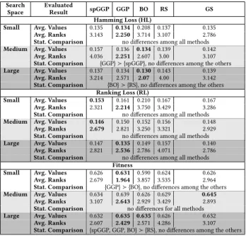
Table 2 shows the average values, the average ranks and the final statistical analysis for HL, RL and fitness measures, respectively.

Table 2: Comparison of the hamming loss (to be minimized), ranking loss (to be minimized) and fitness (to be maximized) obtained by allsearch methodsin the test set for the three designedsearch spaceswith five hours of execution.

Search Space

Evaluated

Result spGGP GGP BO RS GS Hamming Loss (HL)

Small Avg. Values 0.135 0.134 0.208 0.137 0.135

Avg. Ranks 3.143 2.250 3.714 3.107 2.786

Stat. Comparison no differences among all methods

Medium Avg. Values 0.157 0.136 0.134 0.139 0.142

Avg. Ranks 4.036 2.251 2.607 3.00 3.107

Stat. Comparison {GGP}≻{spGGP}, no differences among the others

Large Avg. Values 0.137 0.134 0.130 0.143 0.139

Avg. Ranks 3.214 2.571 2.07 4.00 3.142

Stat. Comparison {BO}≻{RS}, no differences among the others

Ranking Loss (RL)

Small Avg. Values 0.153 0.161 0.210 0.167 0.167

Avg. Ranks 2.321 2.214 3.750 3.429 3.286

Medium Avg. Values 0.146 0.150 0.152 0.156 0.148

Avg. Ranks 2.679 2.821 3.250 3.321 2.929

Large Avg. Values 0.147 0.135 0.149 0.157 0.140

Avg. Ranks 2.821 2.536 2.786 4.071 2.786

Fitness

Small Avg. Values 0.626 0.631 0.590 0.624 0.626

Avg. Ranks 2.679 1.964 3.857 3.535 2.964

Stat. Comparison {GGP}≻{BO}, no differences among the others

Medium Avg. Values 0.634 0.639 0.626 0.629 0.645 Avg. Ranks 3.107 2.643 2.929 3.429 2.893

Stat. Comparison no differences for all methods

Large Avg. Values 0.632 0.635 0.635 0.626 0.632

Avg. Ranks 2.607 2.429 2.571 4.286 3.107

Stat. Comparison {spGGP, GGP, BO}≻{RS}, no differences among the others

The results for the HL measure with five hours, in Table 2, showed that Auto-MEKA𝐺𝐺𝑃had the best average values and ranks

in thesearch spaceSmall, but it had only the best average rank in

thesearch spaceMedium. In addition, Auto-MEKA𝐵𝑂obtained the

best average value and Auto-MEKA𝐺𝐺𝑃 was statistically better

than Auto-MEKA𝑠𝑝𝐺𝐺𝑃in thesearch spaceMedium. Nonetheless,

there is no indication of statistical difference for the other cases of

search spaceMedium, neither for any cases of Small. On the other

hand, when considering thesearch spaceLarge, Auto-MEKA𝐵𝑂had

the best average value and the best average rank. By looking at the statistical results of HL in Table 2, we can observe that only Auto-MEKA𝐵𝑂was able to significantly outperform Auto-MEKA𝑅𝑆 for

thesearch spaceLarge. In the other cases, we do not see an

indi-cation of thesearch methodsto trade-off well between exploration and exploitation. Therefore, based on these HL results, we can con-clude that the size of thesearch spacehas a strong influence on the performance of thesearch method.

4_{We did not present and analyze the results of exact match and}_𝐹

1Macro averaged by

(8)

In addition, Table 2 summarizes the results for the evaluation measure from a different evaluation context, i.e., RL. Whilst Auto-MEKA𝑠𝑝𝐺𝐺𝑃was thesearch methodwith the best average value

in thesearch spaceSmall, Auto-MEKA𝐺𝐺𝑃achieved the best

aver-age rank in this scenario. Distinctly, Auto-MEKA𝑠𝑝𝐺𝐺𝑃selected

and configured MLC algorithms in a way that produced the best average value and rank in thesearch spaceMedium. For thesearch

spaceLarge, Auto-MEKA𝐺𝐺𝑃was thesearch methodwith the best

average value and the best average rank.

The results of RL did not present any evidence of statistical significance. Hence, thesearch methodsdid not differ from each other. As this metric comes from another context, we would like to understand why it presented such a flat result for allsearch

spacesandsearch methods. We believe that the RL measure is very

conservative and it is not sensitive to different choices of multi-label classifiers. As it only penalizes reversed pairs of multi-labels into the ranking and it does not take into account the label-pair depth into the ranking to penalize, this can make this measure not good enough to be used in isolation to evaluate MLC algorithms. In future work, it might be interesting to evaluate whether this measure is appropriate to be part of our study or whether we should consider a rank-based measure that takes into account the depth of the ranking.

HL and RL are measures that compose the fitness/quality func-tion. We also analyze the results of the fitness measure to have a better assessment of the results ofsearch methods. In the last part of Table 2, we show the results for this measure. With re-spect to thesearch spaceSmall, Auto-MEKA𝐺𝐺𝑃presented the best

average value and also the best average rank. Besides, we found statistical evidence that Auto-MEKA𝐺𝐺𝑃 has better results than

Auto-MEKA𝐵𝑂in thissearch space. In thesearch spaceMedium, we

observe that Auto-MEKA𝐺𝐺𝑃produced the best average ranking

and Auto-MEKA𝐺𝑆presented the best average value. Finally, in the

comparison regarding thesearch spaceLarge, Auto-MEKA𝑠𝑝𝐺𝐺𝑃,

Auto-MEKA𝐺𝐺𝑃and Auto-MEKA𝐵𝑂achieved significantly better

results than Auto-MEKA𝑅𝑆, showing their capabilities to handle

enormoussearch spacesś when giving enough time for them to proceed with their searches. Apart from the statistical results, we can observe in Table 2 that Auto-MEKA𝐺𝐺𝑃also reached the best

average value and rank within five hours of running. Furthermore, Auto-MEKA𝐵𝑂had even results to Auto-MEKA𝐺𝐺𝑃in terms of the

average value.

We can now provide overall conclusions based on the results of this section, specially on the fitness measure. We believe that the size of thesearch spacesexplored/exploited by thesearch methods

influenced the accuracy of the MLC predictions. We understand that, for smallersearch spaces(i.e., Small and Medium), thesearch

methodsfind it easier to proceed with their searches and, hence,

their results become broadly similar among each other. When we increase thesearch spaceto Large, only those with robust search mechanisms could deal better with the trade-off between explo-ration and exploexplo-ration, making them achieve competitive results.

However, we believe the robust methods (i.e., those based on the evolutionary and Bayesian optimization frameworks) can still improve their final predictive performances as they could not beat the greedysearch method, a pure-exploitation method. They also face challenges to beat the randomsearch methodin some of the an-alyzed cases. Thus, thesesearch methodsstill could not satisfactorily balance between exploration and exploitation. In our perspective,

this would occur if they could beat simultaneously Auto-MEKA𝑅𝑆

and Auto-MEKA𝐺𝑆. For thesearch spacesSmall and Medium, this

result is more understandable. The smaller thesearch space, the easier it is to perform the search on it. This leads to better results for Auto-MEKA𝑅𝑆and Auto-MEKA𝐺𝑆in such a way that the other

search methodswere not statistically different from both of them.

For biggersearch spaces(i.e., Large), this should be the opposite. As they have robust search mechanisms, they should obtain statisti-cally better results against pure-exploration and pure-exploitation

search methods.

5.2 Analysis of the Diversity of the Selected

Algorithms

We also analyzed the diversity of the MLC algorithms and meta-algorithms selected by the five AutoMLCsearch methods. We focus only on the selected MLC algorithms and meta-algorithms (which are the łmacro-components”), and not on their selected SLC algo-rithms and hyper-parameter settings (the łmicro-components”), to simplify our analysis.

It is important to emphasize that, by analyzing the MLC and SLC algorithms and meta-algorithms selected by allsearch methodsin

eachsearch space, we can better understand the results of Table 2.

This would give an idea of how the choice of an MLC algorithm influences the performance of thesearch methods. However, for the sake of simplicity, we perform this analysis only for thesearch

spaceLarge.

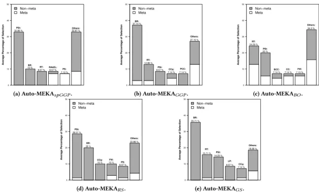
We present in Figures 3b through 3e the bar plots to analyze the relative frequency of selection of MLC algorithms for the AutoMLC

search methods. In these figures we have, for each MLC algorithm,

a bar representing the average relative frequency of selection of an algorithm type over all the 70 runs: 14 datasets times five inde-pendent runs per dataset (five cross-validation folds times one run per fold). We consider two cases: (i) when the traditional MLC algo-rithm is solely selected; (ii) when the traditional MLC algoalgo-rithm is selected together with a MLC meta-algorithm. To emphasize these two cases, the bar for each traditional MLC algorithm is divided into two parts, with sizes proportional to the relative frequency of selection as a standalone algorithm (in gray color) and the relative frequency of selection as part of a meta-algorithm (in white color). Considering this information, BR, PSt and RT were the traditional MLC algorithms most frequently selected by all AutoMLCsearch

methodsin thesearch spaceLarge. BR was chosen, on average,

in 21.43% of all runs for all methods. PSt and RT, in turn, were selected on average in 20.66% and 13.43% of all runs for the five evaluatedsearch methods, respectively. Nevertheless, some of these MLC algorithms were not so present in the selections performed by thesearch methods. For instance, BR and RT were not frequently chosen by Auto-MEKA𝐵𝑂and Auto-MEKA𝑅𝑆. This partially shows

the differences in the selection and configuration of the AutoMLC

search methods, although most of them had similar algorithms at

the top five regarding the ranking of selection.

We can also justify the performance of the methods based on their selection at the MLC meta level. For example, Auto-MEKA𝐺𝐺𝑃

achieved the best results for thesearch spaceLarge in terms of the average value and rank based on fitness, which is the measure we use to decide (for all methods) what algorithm is the most appro-priate. By looking at Auto-MEKA𝐺𝐺𝑃’s selection at the MLC meta

(9)

GECCO ’20, July 8–12, 2020, Cancún, Mexico Non−meta Meta A vera g e P er centa g e of Selection 0 10 20 30 40 50 32.86 % 10 % 8.57 % 8.57 % 7.13 % 32.87 % PSt: BR: RT: RAkEL: PS: Others: (a) Auto-MEKA𝑠𝑝𝐺𝐺𝑃. Non−meta Meta A vera g e P er centa g e of Selection 0 10 20 30 40 50 37.14 % 12.86 % 8.57 % 7.14 % 7.14 % 27.15 % BR: RT: PSt: CCq: PCC: Others: (b) Auto-MEKA𝐺𝐺𝑃. Non−meta Meta A vera g e P er centa g e of Selection 0 10 20 30 40 50 24.29 % 20 % 7.14 % 7.14 % 7.13 % 34.3 % RT: PSt: BCC: CC: FW: Others: (c) Auto-MEKA𝐵𝑂. Non−meta Meta A vera g e P er centa g e of Selection 0 10 20 30 40 50 28.57 % 20 % 10 % 10 % 8.57 % 22.86 % PSt: BR: CCq: FW: PS: Others: (d) Auto-MEKA𝑅𝑆. Non−meta Meta A vera g e P er centa g e of Selection 0 10 20 30 40 50 35.71 % 15.71 % 14.29 % 8.57 % 7.14 % 18.58 % BR: RT: PSt: LP: CCq: Others: (e) Auto-MEKA𝐺𝑆.

Figure 3: Bar plots for the algorithms’ selection frequencies at the MLC level over 70 runs.

Auto-MEKA𝑠𝑝𝐺𝐺𝑃have chosen these MLC meta-algorithms with

a low relative frequency (22.86% for both methods). Therefore, the complexity of the final solution turned them into better options for AutoMLC in the MLC context when contrasted to Auto-MEKA𝐵𝑂,

which selected meta-algorithms in 50% of the cases. However, their level of selection of MLC meta-algorithms is still high when com-pared to Auto-MEKA𝑅𝑆and Auto-MEKA𝐺𝑆, which selected MLC

meta-algorithms in only 10% of the cases. This might be the reason for the competitiveness of Auto-MEKA𝑅𝑆and Auto-MEKA𝐺𝑆.

One test that might be interesting is to remove the MLC meta-algorithms from thesearch space, and reexecute thesearch methods. This could show us whether or not the learned model is more likely to overfit on the training set when we select very complex combinations of base and meta-algorithms. We did that in thesearch

spacesSmall and Medium, but they do not include all traditional

MLC algorithms as thesearch spaceLarge does.

6 CONCLUSIONS

This paper presented an overall comparison among five AutoML

search methodsin the context of multi-label classification ś i.e., Auto-MEKA𝐺𝐺𝑃, Auto-MEKA𝑠𝑝𝐺𝐺𝑃, Auto-MEKA𝐵𝑂, Auto-MEKA𝑅𝑆

and Auto-MEKA𝐺𝑆. To perform this assessment, thesearch methods

were run in 14 MLC datasets with the same execution time budget (i.e., five hours) and in three designedsearch spaces.

The experimental results indicate that Auto-MEKA𝐺𝐺𝑃 is so

far the bestsearch methodas it yields the best predictive results. Besides, it is the only method to be statistically better than Auto-MEKA𝑠𝑝𝐺𝐺𝑃, Auto-MEKA𝐵𝑂and Auto-MEKA𝑅𝑆in different cases.

However, we expected that methods with robust search mecha-nisms (e.g., Auto-MEKA𝑠𝑝𝐺𝐺𝑃, Auto-MEKA𝐵𝑂and Auto-MEKA𝐺𝐺𝑃)

could balance better between exploration and exploitation. This

limitation made these methods not being able to produce statisti-cally better results than Auto-MEKA𝑅𝑆and Auto-MEKA𝐺𝑆, which

are pure-exploration and pure-exploitation methods, respectively. We also observed that the size of thesearch spaceis a crucial issue for the AutoML methods’ behavior. Thus, as a first future work, we intend to better understand the trade-off between parsimony and sufficiency [2]. In other words, we would like to investigate which algorithms should be included to or excluded from thesearch spaces, in order to keep good (combinations of) learning algorithms.

In addition, as two out of the five measures (i.e., FM and RL) yielded flat results, we need to understand how neutral thesearch

spacesare in terms of the chosen MLC performance measures [15,

19]. This would help us to have insights to propose efficient methods or enhancements to thesesearch spaces.

Furthermore, we expect to test other quality criteria to discover appropriate MLC algorithms configurations for a given dataset of interest. This may include finding other relevant performance mea-sures or to set new weights for the current meamea-sures that compose the proposed fitness metric.

Finally, we also plan to include into the proposedsearch methods

a bi-level optimization approach [23] to diminish the hardness of the search in hugesearch spaces. Fundamentally, this would mean to select the learning algorithms in the first place and only configure their hyper-parameters in a second step of the search procedure.

ACKNOWLEDGEMENTS

The authors would like to thank FAPEMIG (through the grant no. CEX-PPM-00098-17), MPMG (through the project Analytical Capabilities), CNPq (through the grant no. 310833/2019-1), CAPES, MCTIC/RNP (through the grant no. 51119) and H2020 (through the grant no. 777154) for their partial financial support.

(10)

REFERENCES

[1] Thomas Back, David B. Fogel, and Zbigniew Michalewicz (Eds.). 1999.

Evolution-ary Computation 2: Advanced Algorithms and Operators(1st ed.). IOP Publishing

Ltd., Bristol, UK.

[2] Wolfgang Banzhaf, Frank D. Francone, Robert E. Keller, and Peter Nordin. 1998.

Genetic Programming: An Introduction. Morgan Kaufmann Publishers Inc., San

Francisco, CA, USA.

[3] Lena Chekina, Lior Rokach, and Bracha Shapira. 2011. Meta-learning for

Se-lecting a Multi-label Classification Algorithm. InProceedings of the International

Conference on Data Mining Workshops (ICDMW’11). IEEE, New York, NY, USA,

220ś227.

[4] Alex G. C. de Sá, Alex A. Freitas, and Gisele L. Pappa. 2018. Automated Selection and Configuration of Multi-Label Classification Algorithms with Grammar-based

Genetic Programming. InProceedings of the International Conference on Parallel

Problem Solving from Nature (PPSN’18). Springer, Cham, Switzerland, 308ś320.

[5] Alex G. C. de Sá, Gisele L. Pappa, and Alex A. Freitas. 2017. Towards a Method for Automatically Selecting and Configuring Multi-Label Classification Algorithms.

InProceedings of the Genetic and Evolutionary Computation Conference Companion

(GECCO’17). ACM, New York, NY, USA, 1125ś1132.

[6] Janez Demšar. 2006. Statistical Comparisons of Classifiers over Multiple Data

Sets.Journal of Machine learning Research7, 1 (2006), 1ś30.

[7] Pedro Domingos. 2012. A Few Useful Things to Know About Machine Learning.

Commun. ACM55, 10 (2012), 78ś87.

[8] Agoston E. Eiben and James E. Smith. 2003.Introduction to Evolutionary

Comput-ing. Vol. 53. Springer, Cham, Switzerland.

[9] Radwa Elshawi, Mohamed Maher, and Sherif Sakr. 2019. Automated Machine Learning: State-of-the-Art and Open Challenges. arXiv preprint, arXiv1906.02287. [10] Eva Gibaja and Sebastián Ventura. 2015. A Tutorial on Multilabel Learning.

Comput. Surveys47, 3 (2015), 52:1ś52:38.

[11] Francisco Herrera, Francisco Charte, Antonio J. Rivera, and María J. Del Jesus.

2016.Multilabel Classification: Problem Analysis, Metrics and Techniques(1st ed.).

Springer, Cham, Switzerland.

[12] Frank Hutter, Holger H. Hoos, and Kevin Leyton-Brown. 2011. Sequential

Model-based Optimization for General Algorithm Configuration. InProceedings

of the International Conference on Learning and Intelligent Optimization (LION’11).

Springer-Verlag, Berlin/Heidelberg, Germany, 507ś523.

[13] Frank Hutter, Lars Kotthoff, and Joaquin Vanschoren (Eds.). 2019.Automated

Machine Learning: Methods, Systems, Challenges. Springer, New York, NY, USA.

Available at http://automl.org/book.

[14] Gjorgji Madjarov, Dragi Kocev, Dejan Gjorgjevikj, and Sašo Džeroski. 2012. An

Extensive Experimental Comparison of Methods for Multi-Label Learning.Pattern

Recognition45, 9 (2012), 3084ś3104.

[15] Katherine M. Malan and Andries P. Engelbrecht. 2013. A Survey of Techniques for

Characterising Fitness Landscapes and Some Possible Ways Forward.Information

Sciences241 (2013), 148ś163.

[16] Robert McKay, Nguyen Hoai, Peter Whigham, Yin Shan, and Michael O’Neill.

2010. Grammar-based Genetic Programming: A Survey.Genetic Programming

and Evolvable Machines11, 3 (2010), 365ś396.

[17] Jose M. Moyano, Eva L. Gibaja, Krzysztof J. Cios, and Sebastián Ventura. 2019. An

Evolutionary Approach to Build Ensembles of Multi-Label Classifiers.Information

Fusion50 (2019), 168ś180.

[18] Rafael B. Pereira, Alexandre Plastino, Bianca Zadrozny, and Luiz H. C. Mer-schmann. 2018. Correlation analysis of performance measures for multi-label

classification.Information Processing and Management54, 3 (2018), 359ś369.

[19] Erik Pitzer and Michael Affenzeller. 2012. A Comprehensive Survey on

Fit-ness Landscape Analysis. InRecent advances in intelligent engineering systems.

Springer-Verlag, Berlin/Heidelberg, Germany, 161ś191.

[20] Jesse Read, Peter Reutemann, Bernhard Pfahringer, and Geoff Holmes. 2016.

MEKA: A Multi-label/Multi-target Extension to WEKA. Journal of Machine

Learning Research17, 21 (2016), 1ś5.

[21] Konstantinos Sechidis, Grigorios Tsoumakas, and Ioannis Vlahavas. 2011. On the

Stratification of Multi-Label Data. InProceedings of the European Conference on

Machine Learning and Principles and Practice of Knowledge Discovery in Databases

(ECML-PKDD’11). Springer-Verlag, Berlin/Heidelberg, Germany, 145ś158.

[22] Eric Siegel. 2013.Predictive Analytics: The Power to Predict Who Will Click, Buy,

Lie, or Die(1st ed.). Wiley Publishing, Hoboken, New Jersey, USA.

[23] El-Ghazali Talbi. 2013. A Taxonomy of Metaheuristics for Bi-Level Optimization.

InMetaheuristics for Bi-Level Optimization. Springer-Verlag, Berlin/Heidelberg,

Germany, 1ś39.

[24] Chris Thornton, Frank Hutter, Holger H. Hoos, and Kevin Leyton-Brown. 2013. Auto-WEKA: Combined Selection and Hyperparameter Optimization of

Classifi-cation Algorithms. InProceedings of the ACM SIGKDD International Conference

on Knowledge Discovery and Data Mining (KDD’13). ACM, New York, NY, USA,

847ś855.

[25] Grigorios Tsoumakas, Ioannis Katakis, and Ioannis Vlahavas. 2010.Mining

Multi-label Data. Springer, Boston, MA, USA, 667ś685.

[26] Grigorios Tsoumakas, Ioannis Katakis, and Ioannis Vlahavas. 2011. Random

k-Labelsets for Multilabel Classification.IEEE Transactions on Knowledge and

Data Engineering23, 7 (2011), 1079ś1089.

[27] Marcel Wever, Felix Mohr, Alexander Tornede, and Eyke Hüllermeier. 2019.

Automating Multi-Label Classification Extending ML-Plan. InProceedings of

the ICML Workshop on Automated Machine Learning (AutoML’19). AutoML.org,

Freiburg, Germany, 1ś8.

[28] Peter A. Whigham. 1995. Grammatically-based Genetic Programming. In

Pro-ceedings of the Workshop on Genetic Programming: From Theory to Real-World

Applications. NRL TR 95.2, University of Rochester, Rochester, New York, USA,

33ś41.

[29] Mohammed J. Zaki and Wagner Meira Jr. 2020. Data Mining and Analysis:

Fundamental Concepts and Algorithms(2nd ed.). Cambridge University Press,

Cambridge, UK.

[30] Min-Ling Zhang and Zhi-Hua Zhou. 2014. A Review on Multi-Label Learning

Algorithms.IEEE Transactions on Knowledge and Data Engineering26, 8 (2014),