C
⃝2015 Biometrika Trust
Printed in Great Britain
Supplementary material for Quantile-based classifiers
B
Y
C. HENNIG
Department of Statistical Science, University College London, London, WC1E 6BT, U.K.
[email protected]
AND
C. VIROLI
5Department of Statistical Sciences, University of Bologna, Bologna, 40126, Italy
[email protected]
1.
T
HEORY FOR
p
= 1
Assuming the notation of Section 2 of the paper, here are some results for
p
= 1
.
The following lemma provides a useful formula to derive the theoretical rate of correct classi-
10fication as function of
θ
for
p
= 1
. This was used for producing Figure 1 of the paper.
L
EMMA
1.
When
p
= 1, the probability of correct classification of the quantile classifier takes
the following simple form:
-
if
q
0(
θ
)
≤
q
1(
θ
),
Ψ(
θ
) =
π
0F
0(¨
q
θ) +
π
1{
1
−
F
1(¨
q
θ)
}
(1)
with
q
¨
θ=
θq
0(
θ
) + (1
−
θ
)
q
1(
θ
);
15-
if
q
0(
θ
)
> q
1(
θ
),
Ψ(
θ
) =
π
1F
1( ˙
q
θ) +
π
0{
1
−
F
0( ˙
q
θ)
}
(2)
with
q
˙
θ=
θq
1(
θ
) + (1
−
θ
)
q
0(
θ
);
where
q
0(
θ
)
and
q
1(
θ
)
are the true quantiles of the two populations.
Proof of Lemma
1
.
In the univariate case
Φ
0(
z, θ
)
and
Φ
1(
z, θ
)
may be rewritten as
20Φ
0(
z, θ
) = (1
−
θ
)
{
q
0(
θ
)
−
z
}
1
{z≤q0(θ)}+
θ
{
z
−
q
0(
θ
)
}
1
{z>q0(θ)},
Φ
1(
z, θ
) = (1
−
θ
)
{
q
1(
θ
)
−
z
}
1
{z≤q1(θ)}+
θ
{
z
−
q
1(
θ
)
}
1
{z>q1(θ)}.
For a fixed
θ, the integral (5) in the paper can be simplified by splitting it into four parts
according to the possible disjoint regions of the domain of
Z
with respect to
q
0(
θ
)
and
q
1(
θ
)
,
namely: (a)
z
≤
min
{
q
0(
θ
)
, q
1(
θ
)
}
, (b)
q
0(
θ
)
< z
≤
q
1(
θ
)
, (c)
q
1(
θ
)
≤
z
≤
q
0(
θ
)
and (d)
z >
max
{
q
0(
θ
)
, q
1(
θ
)
}
.
If
z
≤
min
{
q
0(
θ
)
, q
1(
θ
)
}, case (a), the integral becomes
25Ψ
a(
θ
) =
π
0∫
min{q0(θ),q1(θ)} −∞1
[{1−θ}{q1(θ)−q0(θ)}>0]dP
0(
z
)
+
π
1∫
min{q0(θ),q1(θ)} −∞1
[{1−θ}{q1(θ)−q0(θ)}≤0]dP
1(
z
)
=
π
0∫
q0(θ) −∞dP
0(
z
)
1
{q1(θ)>q0(θ)}+
π
1∫
q1(θ) −∞dP
1(
z
)
1
{q1(θ)≤q0(θ)}=
π
0θ
1
{q1(θ)>q0(θ)}+
π
1θ
1
{q1(θ)≤q0(θ)}.
In case (b) the integral is
Ψ
b(
θ
) =
π
0∫
q1(θ) q0(θ)1
[{1−θ}{q1(θ)−z}−θ{z−q0(θ)}>0]dP
0(
z
)
+
π
1∫
q1(θ) q0(θ)1
[{1−θ}{q1(θ)−z}−θ{z−q0(θ)}≤0]dP
1(
z
)
=
π
0∫
θq0(θ)+(1−θ)q1(θ) q0(θ)dP
0(
z
)
1
{q0(θ)≤q1(θ)}+
π
1∫
q1(θ) θq0(θ)+(1−θ)q1(θ)dP
1(
z
)
1
{q0(θ)≤q1(θ)}.
Similarly, for cases (c) and (d) the integrals are
Ψ
c(
θ
) =
π
0∫
q0(θ) θq1(θ)+(1−θ)q0(θ)dP
0(
z
)
1
{q1(θ)≤q0(θ)}+
π
1∫
θq1(θ)+(1−θ)q0(θ) q1(θ)dP
1(
z
)
1
{q1(θ)≤q0(θ)},
and
Ψ
d(
θ
) =
π
0(1
−
θ
)
1
{q0(θ)>q1(θ)}+
π
1(1
−
θ
)
1
{q0(θ)≤q1(θ)}.
When
q
0(
θ
)
≤
q
1(
θ
)
,
Ψ(
θ
)
is the sum of
Ψ
a(
θ
)
,
Ψ
b(
θ
)
and
Ψ
d(
θ
)
corresponding to disjoint
domain regions of
Z
:
30Ψ(
θ
) =
π
0θ
+
π
0∫
θq0(θ)+(1−θ)q1(θ) q0(θ)dP
0(
z
) +
π
1∫
q1(θ) θq0(θ)+(1−θ)q1(θ)dP
1(
z
) +
π
1(1
−
θ
)
=
π
0θ
+
π
0F
0{θq
0(
θ
) + (1
−
θ
)
q
1(
θ
)
} −
π
0θ
+
π
1θ
−
π
1F
1{θq
0(
θ
) +
+(1
−
θ
)
q
1(
θ
)
}
+
π
1(1
−
θ
) =
π
0F
0(¨
q
θ) +
π
1{
1
−
F
1(¨
q
θ)
}.
Analogously, when
q
0(
θ
)
> q
1(
θ
)
,
Ψ(
θ
)
is the sum of
Ψ
a(
θ
)
,
Ψ
c(
θ
)
and
Ψ
d(
θ
)
, from which
Ψ(
θ
) =
π
1θ
+
π
0∫
q0(θ) θq1(θ)+(1−θ)q0(θ)dP
0(
z
) +
π
1∫
θq1(θ)+(1−θ)q0(θ) q1(θ)dP
1(
z
) +
π
0(1
−
θ
)
=
π
1F
1( ˙
q
θ) +
π
0{
1
−
F
0( ˙
q
θ)
}.
C
OROLLARY
1.
Let
q
(0)(
θ
) = min
{
q
0(
θ
)
, q
1(
θ
)
}
and
q
(1)(
θ
) = max
{
q
0(
θ
)
, q
1(
θ
)
}
. The
probability of correct classification is
Ψ(
θ
) =
π
(0)F
(0)(˜
q
θ) +
π
(1){
1
−
F
(1)(˜
q
θ)
}
,
(3)
where
q
˜
θ=
θq
(0)(
θ
) + (1
−
θ
)
q
(1)(
θ
). The other quantities have been renamed accordingly by
35introducing the notation
l
θ= arg min
k=0,1
{
q
k(
θ
)
}
and
u
θ= arg max
k=0,1{
q
k(
θ
)
}
, from which
F
(0)=
F
lθ,
F
(1)=
F
uθ,
π
(0)=
π
lθand
π
(1)=
π
uθ.
Analogously, the theoretical misclassification rate of the quantile classifier for
p
= 1
is
1
−
Ψ(
θ
) =
π
(0){
1
−
F
(0)(˜
q
θ)
}
+
π
(1)F
(1)(˜
q
θ)
,
(4)
with
q
˜
θ=
θq
(0)(
θ
) + (1
−
θ
)
q
(1)(
θ
).
L
EMMA
2.
Assume that the cumulative distribution functions of the two populations are such
40that the density functions
f
(0)(
z
) =
F
′(0)(
z
)
and
f
(1)(
z
) =
F
′(1)(
z
)
exist for
z
and are nonzero
on the same domain. Further assume that there is a point
z
0with
π
(0)f
(0)(
z
0) =
π
(1)f
(1)(
z
0)
so
that
π
(0)f
(0)(
z
)
> π
(1)f
(1)(
z
)
for
z
on one side of
z
0and
π
(0)f
(0)(
z
)
< π
(1)f
(1)(
z
)
for
z
on the
other side of
z
0. Then the quantile classifier using the quantile
q
˜
θthat minimizes the theoretical
misclassification probability achieves the optimal Bayes misclassification probability.
45Proof of Lemma
2
.
The optimal value
θ
that minimizes the theoretical misclassification
prob-ability in Corollary 1 can be obtained by setting the first derivative of (4) to zero, from which
π
(0)f
(0)(˜
q
θ) =
π
(1)f
(1)(˜
q
θ)
·
A value
θ
exists so that indeed
q
˜
θ=
z
0fulfills this, because under the given assumptions,
q
(0)and
q
(1)are continuous functions of
θ
that converge to the lower and upper bounds of the domain
for
θ
→
0
and
θ
→
1
. Furthermore, under the assumptions of the Theorem, the optimal Bayesian
classifier only has a single decision boundary at
z
0. This proves the Lemma.
2.
A
SYMPTOTIC THEORY
502
·
1
.
Theorem 1
This section contains the proofs of Theorems 1 and 2 of the paper, using the notation of Section
3. The assumptions are:
A1. For all
j
= 1
, . . . , p, k
= 0
,
1
, q
kjis a continuous function of
θ
∈
T
.
A2. For all
θ
∈
T
, pr
[∑
pj=1{
Φ
1j(
Z, θ
)
−
Φ
0j(
Z, θ
)
}
= 0
]
= 0
.
55T
HEOREM
1.
Under A1 and A2, for any
ϵ >
0,
lim
n→∞
pr
{|
Ψ(˜
θ
)
−
Ψ(ˆ
θ
n)
|
> ϵ
}
= 0
.
Proof of Theorem
1
.
The inequality
|
Φ
j(
z, θ
1, q
1)
−
Φ
j(
z, θ
2, q
2)
| ≤ |
z
j||
θ
2−
θ
1|
+ 4
|
q
2−
q
1|
(5)
is proven below for
j
= 1
, . . . , p
as Lemma 3. Together with A1, this implies the continuity of
Ψ
,
because for given
z,
Φ
kjis a continuous function of
θ, and the dominated convergence theorem
The proof of Theorem 1 is now based on the inequality
|
Ψ(˜
θ
)
−
Ψ(ˆ
θ
n)
| ≤ |
Ψ(˜
θ
)
−
Ψ
n(˜
θ
)
|
+
|
Ψ
n(˜
θ
)
−
Ψ
n(ˆ
θ
n)
|
+
|
Ψ
n(ˆ
θ
n)
−
Ψ(ˆ
θ
n)
|.
(6)
In order to show that all three terms on the right side are asymptotically small, the following
result is proved below as Lemma 4.
For all
ϵ >
0 lim
n→∞
pr
{
sup
θ∈T|
Ψ
n(
θ
)
−
Ψ(
θ
)
|
> ϵ
}
= 0
.
(7)
Result (7) forces the first and third term on the right side of (6) to converge to zero in
proba-bility. Now consider the second term. By definition,
65
Ψ
n(ˆ
θ
n)
≥
Ψ
n(˜
θ
)
,
Ψ(˜
θ
)
≥
Ψ(ˆ
θ
n)
.
Using (7) again, for large
n
both
|
Ψ
n(˜
θ
)
−
Ψ(˜
θ
)
|
and
|
Ψ
n(ˆ
θ
n)
−
Ψ(ˆ
θ
n)
|
will be arbitrarily small
with probablity arbitrarily close to 1, and this makes
|
Ψ
n(˜
θ
)
−
Ψ
n(ˆ
θ
n)
|
arbitrarily small, too.
L
EMMA
3.
Equation (
5
) holds for
j
∈ {
1
, . . . , p
}
, θ
1, θ
2∈
(0
,
1)
, q
1, q
2∈
R
under the
as-sumption that (a)
θ
1≤
θ
2and
q
1≤
q
2or (b)
θ
1≥
θ
2and
q
1≥
q
2.
Remark.
If both
q
i(i=1,2) are
θ
i-quantiles of the same distribution, one of (a) or (b) holds.
70
Proof of Lemma
3: Assume (a)
q
1≤
q
2,
0
< θ
1≤
θ
2<
1
; case (b) works by analogy.
Con-sider
z
j≤
q
1, q
1< z
j< q
2, q
2≤
z
jseparately; first
z
j≤
q
1. By definition,
|
Φ
j(
z, θ
1, q
1)
−
Φ
j(
z, θ
2, q
2)
|
=
|
(1
−
θ
1)(
q
1−
z
j)
−
(1
−
θ
2)(
q
2−
z
j)
|
=
|
(
q
1−
q
2) + (
θ
1+
θ
2)(
q
2−
q
1)
−
θ
1q
2+
θ
2q
1+
z
j(
θ
1−
θ
2)
|
≤ |
q
2−
q
1|
+
|
θ
1+
θ
2||
q
2−
q
1|
+
θ
2|
q
2−
q
1|
+
|
z
j(
θ
1−
θ
2)
|
≤ |
z
j||
θ
2−
θ
1|
+ 4
|
q
2−
q
1|
.
For
q
1< z
j< q
2:
|
Φ
j(
z, θ
1, q
1)
−
Φ
j(
z, θ
2, q
2)
|
=
|
θ
1(
z
j−
q
1)
−
(1
−
θ
2)(
q
2−
z
j)
| ≤ |
q
2−
q
1|
.
For
q
2≤
z
j:
|
Φ
j(
z, θ
1, q
1)
−
Φ
j(
z, θ
2, q
2)
|
=
|
θ
1(
z
j−
q
1)
−
θ
2(
z
j−
q
2)
|
,
and (5) follows along the lines of the first case.
75
L
EMMA
4.
Expression (
7
) holds under the conditions of Theorem
1
.
Proof of Lemma
4: Suppose (7) was wrong. This means that there exist
ϵ >
0
, δ >
0
, a
subse-quence
M
of positive integers and
(
θ
∗m)
m∈Msuch that
for all
m
∈
M,
pr
{|
Ψ
m(
θ
∗m)
−
Ψ(
θ
m∗)
|
> ϵ
} ≥
δ.
(8)
Since
(
θ
m)
m∈M∈
T
Mis bounded and at least a subsequence has a limit, there exists
θ
∗=
lim
m→∞θ
∗m.
80
Consider
|
Ψ
m(
θ
m∗)
−
Ψ(
θ
m∗)
| ≤ |
Ψ
m(
θ
m∗)
−
Ψ
m(
θ
∗)
|
+
|
Ψ
m(
θ
∗)
−
Ψ(
θ
∗)
|
+
|
Ψ(
θ
∗)
−
Ψ(
θ
m∗)
|
.
(9)
Regarding the second term, define a version of
Ψ
nusing the true quantiles instead of the
empirical ones:
Ψ
∗n(
θ
) =
1
n
∑
i:Ci=01
p∑
j=1[Φ
j{
Z
i, θ, q
1j(
θ
)
} −
Φ
j{
Z
i, θ, q
0j(
θ
)
}
]
>
0
+
∑
i:Ci=11
p∑
j=1[Φ
j{
Z
i, θ, q
1j(
θ
)
} −
Φ
j{
Z
i, θ, q
1j(
θ
)
}
]
≤
0
.
Consider
85|
Ψ
m(
θ
∗)
−
Ψ(
θ
∗)
| ≤ |
Ψ
m(
θ
∗)
−
Ψ
m∗(
θ
∗)
|
+
|
Ψ
∗m(
θ
∗)
−
Ψ(
θ
∗)
|
.
Because of the strong law of large numbers,
lim
m→∞|
Ψ
∗m(
θ
∗)
−
Ψ(
θ
∗)
|
= 0
almost surely.
For given
z
and
θ,
Φ
jis continuous in
q. Furthermore quantiles are strongly consistent, and
therefore (5) will enforce
lim
m→∞|
Ψ
m(
θ
∗)
−
Ψ
∗m(
θ
∗)
|
= 0
almost surely.
Now consider the first term of the right side of (9).
|
q
kjm(
θ
m∗)
−
q
kjm(
θ
∗)
| ≤ |
q
kjm(
θ
∗)
−
q
kj(
θ
∗)
|
+
|
q
kjm(
θ
∗m)
−
q
kj(
θ
∗m)
|
+
|
q
kj(
θ
m∗)
−
q
kj(
θ
∗)
|
.
(10)
From Theorem 3 in Mason (1982), under assumption A1, we get
lim
m→∞sup
θ∈T|
q
kj(
θ
)
−
90q
kjm(
θ
)
|
= 0
almost surely. This enforces the first two terms on the left side of (10) to converge
to zero almost surely. The last term converges to zero because of A1. Therefore, for
m
→ ∞,
|
q
kjm(
θ
m∗)
−
q
kjm(
θ
∗)
| →
0
almost surely.
(11)
Let
D
n(
θ, z
) =
∑
p j=1{
Φ
1jn(
z, θ
)
−
Φ
0jn(
z, θ
)
},
D
(
θ, z
) =
∑
p j=1{
Φ
1j(
z, θ
)
−
Φ
0j(
z, θ
)
}. For
ϵ >
0
define
Z
ϵ=
{
z
:
|
D
(
θ
∗, z
)
|
> ϵ
} ∩
z
:
p∑
j=1|
z
j| ≤
1
ϵ
,
so that
95|
Ψ
m(
θ
∗m)
−
Ψ
m(
θ
∗)
|
=
1
m
∑
i:Ci=0, Zi̸∈Zϵ[
1
{Dm(θm∗,Zi)>0}−
1
{Dm(θ∗,Zi)>0}]
+
∑
i:Ci=1, Zi̸∈Zϵ[
1
{Dm(θm∗,Zi)≤0}−
1
{Dm(θ∗,Zi)≤0}]
+
∑
i:Ci=0, Zi∈Zϵ[
1
{Dm(θm∗,Zi)>0}−
1
{Dm(θ∗,Zi)>0}]
+
∑
i:Ci=1, Zi∈Zϵ[
1
{Dm(θm∗,Zi)≤0}−
1
{Dm(θ∗,Zi)≤0}]
.
Now for large
m
and arbitrarily small
ν >
0
,
1
m
∑
i:Ci=0, Zi̸∈Zϵ[
1
{Dm(θ∗m,Zi)>0}−
1
{Dm(θ∗,Zi)>0}]
+
∑
i:Ci=1, Zi̸∈Zϵ[
1
{Dm(θ∗m,Zi)≤0}−
1
{Dm(θ∗,Zi)≤0}]
≤
1
−
pr
(
Z
ϵ) +
ν
almost surely.
Furthermore, by (5),
|
D
m(
θ
∗m, Z
i)
−
D
m(
θ
∗, Z
i)
| ≤
p∑
j=1{
2
|
Z
j||
θ
∗m−
θ
∗|
+ 8
|
q
kjm(
θ
m∗)
−
q
kjm(
θ
∗)
|}
.
Because
|
θ
∗m−
θ
∗| →
0
, by (11) and
∑
pj=1|
Z
j| ≤
1
/ϵ
for
Z
∈
Z
ϵ,
|
D
m(
θ
∗m, Z
i)
−
D
m(
θ
∗, Z
i)
|
becomes arbitrarily small almost surely for large enough
m, and therefore for
Z
i∈
Z
ϵ,
D
m(
θ
∗m, Z
i)
and
D
m(
θ
∗, Z
i)
will for large enough
m
be either both positive or both negative,
100
and the corresponding indicator functions will therefore be the same, almost surely.
For
ϵ
↘
0
, assumption A2 enforces pr
(
Z
ϵ)
→
1
. This forces the first term on the right side of
(9) to zero for large
m, almost surely, in contradiction to (8), which in turn proves (7).
2
·
2
.
Theorem 2
The assumptions for Theorem 2 are as follows.
105
B1. The limit
lim
λ→∞sup
k≥1E{|U
k|
1
(|Uk|>λ)}
= 0
.
B2. For each
c >
0
,
inf
k≥1|x
inf
|≥cθinf
∈T(
E
[Φ
k{U, θ, q
k(
θ
) +
x}
]
−
E
[Φ
k{U, θ, q
k(
θ
)
}
])
>
0
.
B3. For each
ϵ >
0
,
inf
k≥1θ
inf
∈T(min[
θ
−
pr
{
U
k≤
q
k(
θ
)
−
ϵ
}
, θ
−
pr
{
U
k≥
q
k(
θ
) +
ϵ
}
])
>
0
.
B4. With
B
denoting the class of Borel subsets of the real line,
lim
k→∞k1,k2:
sup
|k1−k2|≥kB1,B2sup
∈B|pr
(
U
k1∈
B
1, U
k2∈
B
2)
−
pr
(
U
k1∈
B
1)
pr
(
U
k2∈
B
2)
|
= 0
.
B5. The differences
|
ν
Xk,θ−
ν
Y k,θ|
are uniformly bounded.
B6. For sufficiently small
ϵ >
0
, the proportion of values
k
∈
[1
, p
]
for which
|
ν
Xk,θ−
ν
Y k,θ|
>
ϵ
for all
θ
∈
T
is bounded away from zero as
p
diverges.
110
T
HEOREM
2.
Assume B1–B6 hold and that both
n
and
m
diverge as
p
→ ∞
. Then, with
probability converging to 1 as
p
increases, the classifier
R
m,n,pmakes the correct decision, i.e.,
pr
{R
m,n,p(
Z
) = 1
|
C
= 0
}
+
pr
{R
m,n,p(
Z
) = 0
|
C
= 1
} →
0
.
Proof of Theorem
2: In the proof of Theorem 1 in Hall et al. (2009), B2, B3, B5 and B6
en-force every statement to hold uniformly for
θ
∈
T
, after definitions have been adapted to general
quantile classifiers. More specifically,
W
k, D
k, D
(
Z
)
, S
λ, d
(
Z
)
,
K
ϵand
d
kneed to be defined
115
applied and
q
k(
θ
)
replacing zero where B3 is applied. Equations (A.1)–(A.6) in Hall et al. (2009)
then hold uniformly over
T.
Remark
1
.
We expect that similar arguments can be used to prove a version of Theorem 2 in
Hall et al. (2009), which has different assumptions, for the quantile classifier.
1203.
D
ETAILED RESULTS OF THE SIMULATION STUDY
3·1
.
Software information and tuning parameters
The package
quantileDA
available on CRAN/R computes quantile, median and centroid
classifiers.
The implementation of the classification methods used for comparison has been done with
125the following software and parameter choices. We used the R package
MASS
to implement
Fisher’s LDA and the package
pamr
for the nearest-shrunken centroid. The
k-nearest-neighbor
classifier has been run under the library
class
with a number of neighbors,
k, chosen
be-tween 1 and 9 by cross-validation in the training set. For the support vector machine we used
the library
e1071
with the combination of tuning parameters
γ
= (0
·
001
,
0
·
01
,
0
·
1
,
1
,
2)
and
130Cost
= (1
,
2
,
4
,
8
,
16)
optimized in each dataset according to the function
tune.svm
. For
the classification trees we used the package
rpart
with the combination of tuning
parame-ters
minsplit
= (5
,
10
,
15
,
20)
and
cp
= (0
·
001
,
0
·
01
,
0
·
1
,
0
·
2)
selected by cross-validation.
The naive Bayes classifier has been fitted by the package
klaR
with kernel estimate
densi-ties instead of Gaussian densidensi-ties in order to gain flexibility. We used the package
stepPlr
135for penalized logistic regression with regularization parameter,
λ, chosen by cross-validation in
λ
= (0
·
00001
,
0
·
0001
,
0
·
001
,
0
·
01
,
0
·
1
,
1)
.
3
·
2
.
Classification results
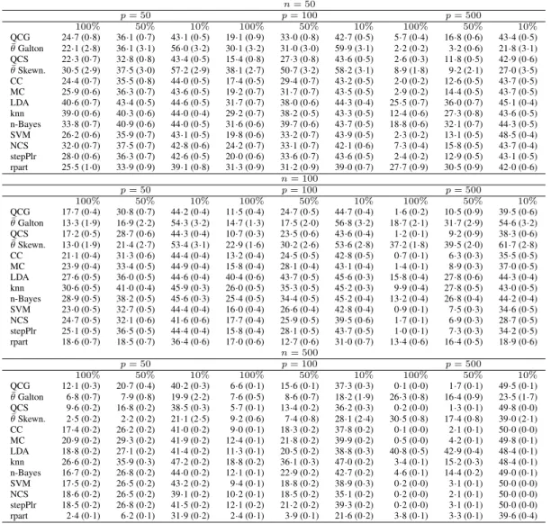
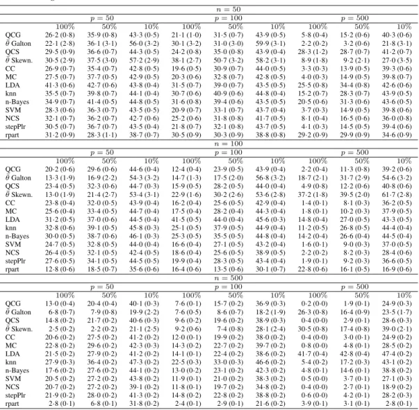
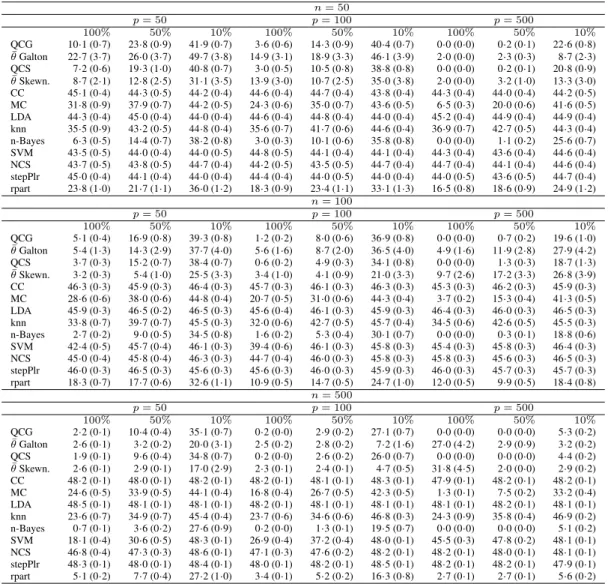
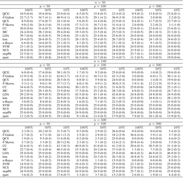
The tables show the average misclassification rates multiplied by 100 and the average of the
optimal
θ
values across all the 100 data sets in each setting considered. Standard errors are re-
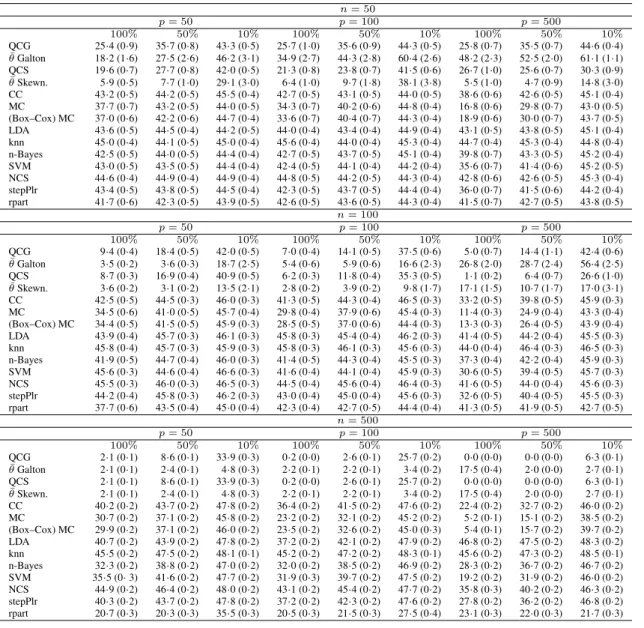
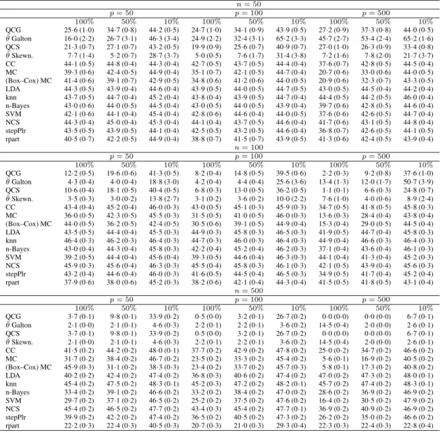
140ported in brackets. Tables 3 and 4 also report the misclassification rates obtained by the median
classifier on data preprocessed by the Box–Cox power transformation in order to check whether
this transformation could improve the classification performance of the median classifier by
re-ducing the skewness of variables. For each variable, we considered 100 values equally spaced in
the interval
[
−
2
,
2]
for the Box–Cox parameter, and the single parameter value that maximized
145the profile log-likelihood of a Gaussian distribution for each variable was selected in the training
set and applied to the test set. The Box–Cox transformation does not improve the classification
performance, because the most discriminative information between the two classes in the tails of
the class distributions still remains located in the tails even if the distributional shape changes.
R
EFERENCES
150H
ALL, P., T
ITTERINGTON, D. M. & X
UE, J. H. (2009). Median-based classifiers for high-dimensional data.
Journal
of the American Statistical Society
104
, 1597–1608.
M
ASON, D. M. (1982). Some Characterizations of Almost Sure Bounds for Weighted Multidimensional Empirical
Distributions and a Glivenko–Cantelli Theorem for Sample Quantiles.
Zeitschrift fuer Wahrscheinlichkeitstheorie
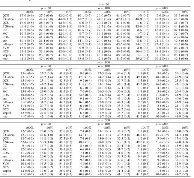
Table 1.
Simulation study: independent identically distributed symmetric variables.
Misclassifi-cation rates multiplied by 100 (with standard errors in brackets; all rounded to one digit after
the decimal point) for different methods. Rows 2 and 4 contain the mean of the chosen values of
θ
in the training sets.
n= 50 p= 50 p= 100 p= 500 100% 50% 10% 100% 50% 10% 100% 50% 10% QCG 17·0(0·6) 27·5(0·6) 42·2(0·6) 10·1(0·5) 20·0(0·7) 41·2(0·7) 1·5(0·2) 5·6(0·4) 31·5(0·8) ¯ θGalton 46·1(1·8) 44·4(1·8) 44·3(1·7) 45·7(1·3) 44·0(1·4) 42·7(1·1) 48·3(0·3) 48·3(0·2) 48·3(0·3) QCS 16·6(0·8) 28·3(0·7) 42·5(0·6) 9·6(0·6) 20·7(0·7) 41·1(0·6) 1·6(0·2) 5·8(0·3) 31·4(0·7) ¯ θSkewn. 49·4(1·0) 41·3(1·8) 42·9(1·9) 39·5(1·2) 42·7(1·5) 43·6(1·5) 42·8(0·6) 43·1(0·3) 44·1(0·3) CC 16·2(0·8) 27·3(0·7) 43·1(0·5) 10·5(0·7) 22·0(1·0) 41·9(0·6) 3·5(0·8) 13·3(1·4) 37·1(0·8) MC 16·5(0·5) 26·9(0·6) 42·1(0·5) 9·7(0·5) 19·3(0·6) 41·9(0·5) 1·7(0·2) 6·4(0·4) 32·0(0·7) LDA 37·5(0·7) 41·2(0·7) 43·5(0·5) 22·8(0·7) 30·4(0·7) 42·7(0·5) 26·0(0·9) 35·8(0·8) 43·2(0·5) knn 19·1(0·7) 31·1(0·8) 44·2(0·4) 14·1(0·7) 29·0(0·8) 43·4(0·6) 5·6(0·7) 21·1(1·3) 42·8(0·6) n-Bayes 26·7(0·7) 35·5(0·8) 43·3(0·5) 20·2(0·7) 33·2(0·8) 43·5(0·5) 14·1(0·9) 27·4(1·0) 43·4(0·5) SVM 18·0(0·9) 25·6(0·8) 42·6(0·5) 9·9(0·5) 17·5(0·5) 43·1(0·4) 3·9(0·3) 5·9(0·5) 26·7(0·7) NCS 29·4(0·8) 36·3(0·8) 42·0(0·6) 23·0(0·7) 31·2(0·8) 40·7(0·6) 10·4(0·6) 18·4(0·8) 36·3(0·8) stepPlr 14·7(0·5) 23·5(0·7) 41·8(0·6) 6·9(0·4) 15·3(0·5) 38·3(0·6) 1·1(0·1) 3·1(0·3) 25·1(0·7) rpart 41·3(0·6) 42·4(0·6) 44·3(0·4) 38·8(0·6) 42·1(0·5) 41·7(0·6) 39·2(0·6) 39·2(0·6) 42·1(0·6) n= 100 p= 50 p= 100 p= 500 100% 50% 10% 100% 50% 10% 100% 50% 10% QCG 15·4 (0·4) 25·2 (0·5) 41·9 (0·4) 9·3 (0·4) 17·5 (0·4) 39·6 (0·5) 1·4 (0·1) 3·8 (0·2) 26·1 (0·4) ¯ θGalton 43·3 (1·5) 43·2 (1·6) 42·2 (1·5) 47·0 (1·8) 44·2 (1·6) 43·8 (1·3) 49·1 (0·5) 48·2 (0·4) 47·9 (0·5) QCS 15·5 (0·4) 25·1 (0·4) 42·5 (0·4) 9·7 (0·4) 17·8 (0·5) 39·7 (0·5) 1·5 (0·1) 3·9 (0·2) 25·5 (0·4) ¯ θSkewn. 43·5 (1·7) 47·2 (1·6) 46·9 (1·9) 41·9 (1·7) 45·1 (1·6) 47·1 (1·4) 45·5 (0·5) 46·1 (0·3) 47·1 (0·5) CC 13·0 (0·6) 21·8 (0·6) 42·4 (0·5) 6·7 (0·3) 16·1 (0·6) 37·4 (0·6) 1·0 (0·1) 4·4 (0·5) 30·1 (0·8) MC 13·8 (0·4) 23·0 (0·5) 41·5 (0·5) 7·6 (0·3) 16·5 (0·3) 36·6 (0·5) 1·3 (0·1) 3·9 (0·2) 26·4 (0·5) LDA 18·0 (0·5) 27·2 (0·5) 42·6 (0·4) 34·6 (0·8) 38·6 (0·6) 44·7 (0·4) 12·4 (0·4) 21·6 (0·5) 41·9 (0·5) knn 15·3 (0·4) 26·3 (0·5) 43·6 (0·5) 9·1 (0·4) 21·1 (0·7) 43·1 (0·5) 2·1 (0·2) 13·2 (1·0) 40·6 (0·6) n-Bayes 21·2 (0·5) 31·7 (0·6) 44·3 (0·4) 16·3 (0·5) 27·8 (0·7) 44·3 (0·4) 9·6 (0·5) 19·8 (0·9) 41·9 (0·6) SVM 11·8 (0·3) 20·7 (0·4) 41·9 (0·5) 6·9 (0·3) 13·8 (0·3) 35·8 (0·6) 2·6 (0·2) 3·6 (0·2) 21·1 (0·5) NCS 24·8 (0·6) 29·9 (0·5) 41·1 (0·5) 17·4 (0·4) 25·9 (0·6) 38·2 (0·6) 4·4 (0·3) 9·8 (0·4) 28·3 (0·7) stepPlr 12·9 (0·3) 22·5 (0·5) 40·7 (0·4) 6·6 (0·3) 13·9 (0·3) 36·7 (0·5) 0·8 (0·1) 2·3 (0·2) 19·6 (0·4) rpart 41·7 (0·4) 42·1 (0·4) 43·8 (0·5) 41·3 (0·5) 41·7 (0·5) 43·2 (0·5) 41·5 (0·4) 40·0 (0·4) 41·9 (0·4) n= 500 p= 50 p= 100 p= 500 100% 50% 10% 100% 50% 10% 100% 50% 10% QCG 12·7 (0·2) 20·0 (0·2) 37·6 (0·2) 7·1 (0·1) 13·1 (0·1) 32·5 (0·2) 1·2 (0·1) 3·1 (0·1) 17·0 (0·2) ¯ θGalton 42·7 (1·1) 42·6 (1·0) 41·9 (1·0) 44·3 (1·3) 44·3 (1·1) 43·2 (1·0) 48·2 (2·0) 45·2 (1·9) 44·3 (1·0) QCS 12·7 (0·2) 19·8 (0·2) 37·5 (0·3) 7·1 (0·1) 13·0 (0·1) 32·5 (0·2) 1·2 (0·1) 3·0 (0·1) 17·4 (0·2) ¯ θSkewn. 52·6 (1·2) 50·3 (1·0) 48·5 (1·3) 48·4 (1·3) 49·8 (1·2) 50·1 (1·1) 49·3 (1·7) 51·4 (1·7) 49·0 (1·3) CC 9·4 (0·1) 16·7 (0·2) 35·7 (0·3) 5·6 (0·4) 10·0 (0·1) 30·4 (0·2) 0·7 (0·0) 1·8 (0·1) 15·9 (0·6) MC 12·2 (0·2) 19·4 (0·2) 36·3 (0·2) 6·9 (0·1) 12·5 (0·2) 31·7 (0·2) 1·1 (0·0) 2·5 (0·1) 16·2 (0·2) LDA 11·2 (0·2) 18·6 (0·2) 35·7 (0·3) 7·1 (0·1) 12·8 (0·2) 31·6 (0·2) 33·8 (0·6) 37·9 (0·5) 45·5 (0·3) knn 10·8 (0·1) 20·0 (0·2) 41·4 (0·2) 5·8 (0·1) 13·2 (0·2) 39·3 (0·3) 0·9 (0·0) 4·0 (0·2) 31·4 (0·6) n-Bayes 14·2 (0·2) 23·3 (0·3) 41·9 (0·3) 9·8 (0·1) 18·3 (0·3) 39·6 (0·4) 5·3 (0·2) 9·7 (0·4) 35·1 (0·7) SVM 10·8 (0·1) 16·5 (0·2) 34·1 (0·2) 4·9 (0·1) 11·5 (0·1) 30·1 (0·2) 1·4 (0·1) 2·5 (0·1) 12·9 (0·2) NCS 11·7 (0·2) 18·8 (0·2) 33·3 (0·3) 7·0 (0·3) 11·7 (0·2) 28·0 (0·2) 1·0 (0·0) 2·4 (0·1) 12·7 (0·2) stepPlr 12·0 (0·2) 19·0 (0·2) 36·0 (0·2) 6·6 (0·1) 13·8 (0·2) 31·4 (0·2) 0·7 (0·0) 1·8 (0·1) 14·3 (0·2) rpart 41·2 (0·2) 41·2 (0·3) 41·4 (0·2) 40·9 (0·2) 41·5 (0·2) 41·1 (0·2) 41·5 (0·3) 40·9 (0·2) 41·2 (0·2)
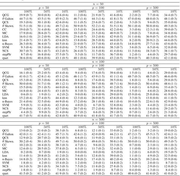
Table 2.
Simulation study: dependent identically distributed symmetric variables.
Misclassifica-tion rates multiplied by 100 (with standard errors in brackets; all rounded to one digit after the
decimal point) for different methods. Rows 2 and 4 contain the mean of the chosen values of
θ
in the training sets.
n= 50 p= 50 p= 100 p= 500 100% 50% 10% 100% 50% 10% 100% 50% 10% QCG 19·9 (0·7) 30·0 (0·8) 42·6 (0·6) 11·2 (0·6) 21·9 (0·7) 41·6 (0·6) 2·2 (0·2) 7·7 (0·4) 34·4 (0·7) ¯ θGalton 44·7 (1·9) 43·5 (1·9) 45·9 (2·3) 46·7 (1·4) 44·3 (1·6) 41·8 (1·5) 47·0 (0·6) 48·0 (0·3) 48·1 (0·3) QCS 19·3 (0·6) 30·1 (0·8) 42·6 (0·6) 11·1 (0·5) 23·6 (0·7) 41·2 (0·6) 3·3 (0·3) 9·6 (0·5) 35·0 (0·6) ¯ θSkewn. 51·5 (1·0) 50·1 (1·6) 49·7 (2·4) 50·9 (0·5) 52·2 (1·4) 51·5 (1·8) 50·1 (0·4) 50·8 (0·6) 49·3 (0·3) CC 19·0 (0·7) 31·4 (0·8) 42·5 (0·6) 13·5 (0·9) 24·6 (0·9) 42·2 (0·6) 3·3 (0·6) 12·3 (1·0) 39·0 (0·7) MC 17·9 (0·6) 28·6 (0·7) 42·0 (0·6) 10·3 (0·4) 21·5 (0·6) 40·9 (0·7) 2·0 (0·2) 7·8 (0·4) 34·8 (0·6) LDA 16·0 (1·0) 21·2 (0·9) 36·2 (0·9) 23·6 (0·7) 33·2 (0·8) 42·9 (0·5) 31·1 (0·8) 36·9 (0·7) 43·6 (0·5) knn 21·4 (0·7) 33·1 (0·7) 43·6 (0·5) 13·8 (0·6) 28·5 (0·8) 44·0 (0·5) 8·2 (0·9) 20·9 (1·2) 44·6 (0·5) n-Bayes 26·3 (0·8) 36·4 (0·7) 44·5 (0·4) 21·0 (0·7) 33·7 (0·8) 43·4 (0·5) 14·8 (0·9) 27·7 (1·0) 43·6 (0·5) SVM 9·3 (0·4) 18·3 (0·6) 41·0 (0·6) 7·7 (0·5) 14·8 (0·6) 38·3 (0·7) 3·6 (0·3) 6·5 (0·4) 32·8 (0·8) NCS 30·7 (0·7) 36·1 (0·7) 43·2 (0·5) 26·4 (0·7) 31·5 (0·8) 41·4 (0·6) 11·3 (0·6) 18·3 (0·7) 38·1 (0·7) stepPlr 8·7 (0·4) 16·8 (0·6) 37·5 (0·7) 5·3 (0·3) 11·7 (0·5) 36·7 (0·8) 1·2 (0·1) 4·6 (0·3) 29·7 (0·6) rpart 38·6 (0·6) 40·6 (0·6) 43·1 (0·5) 40·1 (0·6) 39·9 (0·6) 43·2 (0·5) 39·0 (0·7) 40·3 (0·6) 42·1 (0·6) n= 100 p= 50 p= 100 p= 500 100% 50% 10% 100% 50% 10% 100% 50% 10% QCG 16·1 (0·4) 25·2 (0·5) 43·4 (0·4) 9·4 (0·4) 17·6 (0·5) 39·6 (0·6) 1·5 (0·1) 4·6 (0·2) 29·0 (0·4) ¯ θGalton 41·0 (1·7) 42·8 (1·4) 45·1 (2·0) 46·1 (1·7) 43·9 (1·5) 41·1 (1·4) 48·7 (0·3) 48·5 (0·7) 46·6 (0·9) QCS 15·3 (0·4) 25·3 (0·6) 43·8 (0·4) 8·8 (0·3) 17·6 (0·4) 39·5 (0·6) 1·8 (0·1) 5·6 (0·4) 29·8 (0·5) ¯ θSkewn. 50·0 (0·6) 51·7 (1·0) 49·1 (2·1) 49·9 (0·4) 50·7 (0·8) 48·7 (1·6) 50·0 (0·2) 50·4 (0·6) 48·6 (1·1) CC 15·5 (0·6) 25·1 (0·5) 44·0 (0·4) 8·8 (0·5) 18·6 (0·7) 41·2 (0·5) 1·4 (0·1) 6·9 (0·6) 33·4 (0·7) MC 14·8 (0·4) 24·4 (0·5) 43·1 (0·5) 8·3 (0·3) 16·4 (0·4) 39·4 (0·6) 1·5 (0·1) 4·6 (0·2) 28·6 (0·4) LDA 0·6 (0·1) 1·9 (0·1) 4·2 (0·2) 9·0 (0·8) 11·9 (0·9) 29·0 (0·9) 15·9 (0·4) 25·8 (0·6) 41·9 (0·5) knn 15·2 (0·4) 27·4 (0·5) 44·4 (0·4) 12·3 (0·4) 26·0 (0·5) 43·6 (0·4) 3·3 (0·3) 13·8 (0·8) 41·1 (0·5) n-Bayes 21·4 (0·6) 32·5 (0·6) 44·9 (0·4) 17·2 (0·6) 28·1 (0·8) 44·1 (0·4) 10·4 (0·5) 22·6 (1·0) 42·9 (0·6) SVM 5·9 (0·3) 11·4 (0·4) 42·3 (0·4) 4·0 (0·2) 6·7 (0·3) 32·8 (0·6) 2·3 (0·2) 4·4 (0·2) 23·4 (0·5) NCS 27·6 (0·6) 32·1 (0·5) 42·7 (0·6) 20·7 (0·4) 27·2 (0·6) 38·9 (0·6) 6·4 (0·3) 11·6 (0·4) 29·2 (0·7) stepPlr 4·4 (0·2) 9·9 (0·3) 21·4 (0·6) 3·7 (0·2) 6·6 (0·3) 29·1 (0·5) 0·7 (0·1) 2·6 (0·2) 21·3 (0·4) rpart 41·7 (0·5) 41·6 (0·4) 42·8 (0·5) 40·9 (0·4) 41·8 (0·5) 41·7 (0·5) 39·0 (0·4) 41·7 (0·5) 41·9 (0·5) n= 500 p= 50 p= 100 p= 500 100% 50% 10% 100% 50% 10% 100% 50% 10% QCG 13·0 (0·2) 21·0 (0·2) 38·3 (0·3) 6·8 (0·1) 12·1 (0·1) 33·0 (0·2) 1·2 (0·1) 3·2 (0·1) 19·0 (0·2) ¯ θGalton 42·0 (1·1) 42·4 (1·1) 45·7 (1·3) 42·6 (1·2) 42·0 (0·9) 44·2 (1·1) 47·2 (1·7) 45·5 (1·7) 42·6 (1·1) QCS 12·9 (0·2) 20·7 (0·2) 38·4 (0·3) 6·6 (0·1) 11·9 (0·2) 33·1 (0·3) 1·2 (0·1) 3·1 (0·1) 18·5 (0·2) ¯ θSkewn. 50·2 (0·4) 50·1 (0·5) 49·7 (1·4) 50·0 (0·2) 49·6 (0·3) 50·8 (1·0) 50·0 (0·1) 50·0 (0·1) 49·5 (0·7) CC 10·2 (0·2) 18·4 (0·3) 38·3 (0·3) 4·7 (0·1) 9·6 (0·2) 33·3 (0·3) 0·7 (0·0) 2·3 (0·1) 19·1 (0·3) MC 12·6 (0·1) 20·5 (0·2) 37·8 (0·2) 6·3 (0·1) 11·7 (0·2) 32·4 (0·2) 1·1 (0·0) 2·9 (0·1) 18·1 (0·2) LDA 0·2 (0·0) 0·7 (0·0) 1·9 (0·1) 0·0 (0·0) 0·0 (0·0) 0·5 (0·0) 1·2 (0·1) 6·0 (0·5) 19·5 (0·7) knn 11·4 (0·1) 20·8 (0·2) 41·2 (0·2) 5·6 (0·1) 12·8 (0·3) 39·0 (0·2) 1·1 (0·1) 4·9 (0·2) 32·5 (0·6) n-Bayes 14·8 (0·2) 23·5 (0·3) 42·8 (0·3) 9·8 (0·2) 17·4 (0·3) 40·2 (0·4) 5·6 (0·2) 10·2 (0·4) 35·9 (0·8) SVM 1·8 (0·1) 4·2 (0·1) 15·4 (0·2) 1·2 (0·0) 2·0 (0·1) 14·8 (0·2) 1·3 (0·1) 2·0 (0·1) 8·7 (0·1) NCS 14·3 (0·3) 20·1 (0·3) 34·3 (0·3) 7·5 (0·2) 11·8 (0·2) 27·8 (0·3) 1·3 (0·1) 2·9 (0·1) 12·8 (0·2) stepPlr 1·8 (0·1) 2·5 (0·1) 7·6 (0·1) 1·2 (0·1) 1·9 (0·1) 8·7 (0·1) 0·4 (0·0) 1·3 (0·1) 8·4 (0·1) rpart 41·5 (0·2) 41·2 (0·2) 41·9 (0·3) 41·7 (0·2) 41·5 (0·2) 41·4 (0·2) 40·6 (0·2) 41·6 (0·2) 41·0 (0·2)