Guiding Evolutionary Multi-Objective
Optimization with Generic Front Modeling
Ye Tian, Xingyi Zhang, Ran Cheng, Cheng He, and Yaochu Jin,
Fellow, IEEE
Abstract—In evolutionary multi-objective optimization, the Pareto front is approximated using a set of representative candidate solutions with good convergence and diversity. However, most existing multi-objective evolutionary algo-rithms have general difficulty in the approximation of Pareto fronts with complicated geometries. To address this issue, we propose a generic front modeling method for evolutionary multi-objective optimization, where the shape of the non-dominated front is estimated by training a generalized simplex model. On the basis of the estimated front, we further develop a multi-objective evolutionary algorithm, where both the mating selection and environmental selec-tion are driven by the approximate non-dominated fronts modeled during the optimization process. For performance assessment, the proposed algorithm is compared with several state-of-the-art evolutionary algorithms on a wide range of benchmark problems with various types of Pareto fronts and different numbers of objectives. Experimental results demon-strate that the proposed algorithm performs consistently on a variety of multi-objective optimization problems.
Index Terms—Evolutionary algorithm, multi- and many-objective optimization, front modeling, fitness function
I. INTRODUCTION
M
ULTI-objective optimization problems (MOPs)of-ten involve two or more conflicting objectives to be optimized simultaneously, which widely exist in real-world applications [1], [2]. When the number of objectives is larger than three, MOPs are also known as many-objective optimization problems (MaOPs) [3]. Since there does not exist a single solution that optimizes
Manuscript received –. This work was supported in part by the National Natural Science Foundation of China under Grant 61822301, Grant 61672033, Grant 61502004, and Grant 61502001, Anhui Provin-cial Natural Science Foundation for Distinguished Young Scholars under Grant 1808085J06, and Shenzhen Peacock Plan under Grant KQTD2016112514355531. The work of Y. Jin was supported in part by the U.K. EPSRC under Grant EP/M017869/1. (Corresponding authors: Xingyi Zhang and Ran Cheng)
Y. Tian is with the Institute of Physical Science and Informa-tion Technology, Anhui University, Hefei 230601, China (email: [email protected]).
X. Zhang is with the Institute of Bio-inspired Intelligence and Min-ing Knowledge, School of Computer Science and Technology, Anhui University, Hefei 230039, China (email: [email protected]).
R. Cheng and C. He are with the Shenzhen Key Laboratory of Computational Intelligence, University Key Laboratory of Evolving Intelligent Systems of Guangdong Province, Department of Com-puter Science and Engineering, Southern University of Science and Technology, Shenzhen 518055, China (email: [email protected]; [email protected]).
Y. Jin is with the Department of Computer Science, University of Sur-rey, Guildford, SurSur-rey, GU2 7XH, U.K. (email: [email protected]).
all conflicting objectives, it is usually expected that a set of solutions will be obtained as trade-offs between different objectives. All the trade-off solutions, known as Pareto optimal solutions, constitute the Pareto set (PS), and the image of the PS in objective space is known as the Pareto front (PF) [4].
Over the last two decades, the multi-objective evolu-tionary algorithms (MOEAs) have demonstrated high ef-fectiveness in solving MOPs [4]. In terms of the environ-mental selection strategies, the existing MOEAs can be roughly classified into three categories, i.e., Pareto domi-nance based MOEAs, decomposition based MOEAs, and indicator based MOEAs. The Pareto dominance based MOEAs utilize the non-dominated sorting approaches [5] to divide candidate solutions into several fronts at the first stage, and afterwards distinguish the candidate solutions in the same front by other diversity metrics [6], [7]. The decomposition based MOEAs are characterized by decomposing the original MOP into a number of single-objective optimization problems (SOPs) or simpler MOPs to be solved in a collaborative manner [8], [9]. As for the indicator based MOEAs, where the environ-mental selection is based on a performance indicator such as hypervolume [10], inverted generational distance [11], and R2 [12], the fitness of a candidate solution is measured by its contribution to the indicator value with respect to the whole population [13], [14].
As reported in some recent studies [15], [16], despite that evolutionary multi-objective optimization has been widely verified on a variety of benchmark problems, it is still a challenging task to maintain a good distribution of the candidate solutions on various types of irregular PFs. For example, in decomposition based MOEAs, since the predefined weight vectors are uniformly sampled on the unit hyperplane, the candidate solutions distributed in the middle of convex/concave PFs will be more/less crowded than those on the border, and such a phe-nomenon can become worse when the PF has a sharp peak or long tail [17]. Besides, since the distribution of the candidate solutions is mostly determined by the predefined weight vectors, the difference between the PF shape and the distribution of weight vectors could also lead to a substantial deterioration of the performance of decomposition based MOEAs [15]. Similar issues could also exist in indicator (e.g. hypervolume [10]) based MOEAs [13], [18], where the candidate solutions have
biased distribution in the middle of a convex/concave PF due to their larger/smaller hypervolume contributions than those on the borders.
To address the above issues, some approaches were proposed to enhance the performance consistency of MOEAs for tackling MOPs with various PFs, for in-stance, the adaptive parameter setting based approaches [19], [20] and the weight vector adaptation based ap-proaches [17], [21]. However, little work has been dedi-cated to direct modeling the geometrical structures of the PFs. Intuitively, if an MOEA is able to model the PF of a given MOP, the algorithm can ideally make selections among candidate solutions with respect to the modeled PF, regardless of the specific PF shape. Motivated by this, we propose a generic front modeling based MOEA for enhancing the performance consistency of MOEAs in solving MOPs with various PFs, where the contributions of this paper can be summarized as follows:
1) A generic front modeling (GFM) method is pro-posed for estimating the PF of a given MOP by iteratively training a generalized simplex model. In the proposed GFM method, the non-dominated solutions obtained during the optimization process are used as the training data, and the Levenberg-Marquardt algorithm is employed to estimate the parameters of the model by minimizing the train-ing error. As demonstrated by the examples given in Section III-B, the proposed GFM can estimate various types of PFs with low errors.
2) An evolutionary algorithm (called GFM-MOEA) is developed on the basis of GFM, where both mating selection and environmental selection are driven by the estimated PF models. To be specific, a novel fitness function is proposed as the selection criterion, where the convergence quality of a can-didate solution is measured by its distance to the estimated PF, while the diversity quality is mea-sured by its projection on the estimated PF model. Experimental results demonstrate the effectiveness of the proposed GFM-MOEA on MOPs and MaOPs with various types of PFs.
The rest of this paper is organized as follows. In Section II, we briefly review some existing MOEAs for enhancing the performance consistency and MOEAs based on PF modeling. The proposed GFM method is elaborated in Section III, followed by the description of GFM-MOEA in Section IV. Experimental results and discussions are given in Section V. Lastly, conclusions are drawn in Section VI.
II. RELATEDWORK
A. MOEAs for Enhancing the Performance Consistency in Solving MOPs with Various PFs
There are a large number of MOEAs developed to enhance the performance consistency in solving MOPs with various PFs [17], [19]–[25], which can be roughly grouped into the following three categories.
The first category is motivated to deal with scaled ob-jectives by normalizing the objective values. For MOEAs in this category, the objective values of all the candidate solutions in the population are usually normalized ac-cording to the intercept of each axis and the hyperplane constructed by the extreme solutions [26]. NSGA-III [9],
I-DBEA [27] and θ-DEA [28], which show consistent
performance on MOPs with badly-scaled PFs, are three representative MOEAs belonging to this category.
The second category aims to adapt the fitness function to match the PF shape. Take MOEA/D-PaS [20] as an example, where the performance of decomposition based MOEAs is enhanced using a Pareto adaptive scalarizing
method. Specifically, MOEA/D-PaS uses a weightedLp
scalarizing method as the aggregation function, where the weighted sum and Tchebycheff methods are special cases ofLpwhenp= 1andp=∞, respectively. Then the
algorithm finds thepvalue for each weight vector such
that the optimal solution identified by the associatedLp scalarizing method is the closest one to the weight vector.
In this way, the contour curve of the Lp scalarizing
method can approximate the curvature of the true PF, and thus lead to the consistent performance on problems with various PF shapes.
The third category applies weight vector adaptation, e.g., A-NSGA-III [9], MOEA/D-AWA [17], and RVEA* [21], where the basic idea is to adjust the distribution of the weight vectors according to the candidate solu-tions in the current population or an external archive. Normally, the initial weight vector set has a simplex-like distribution, while the adapted weight vector set can have a distribution similar to the PF shape, hence enhancing the performance of the MOEAs to achieve the maximum coverage of the PF.
However, due to the various PF shapes of MOPs, most of the above algorithms have limitations in solving MOPs. On one hand, NSGA-III and MOEA/D-PaS only estimate the rough scales or curvatures of the PFs, which may not work on MOPs with complicated irregular PFs. On the other hand, despite that A-NSGA-III, MOEA/D-AWA, and RVEA* are tailored for MOPs with irregular PFs, they fail to perform consistently on MOPs with regular PFs [25]. In contrast to the above MOEAs, there are some other MOEAs which enhance the performance consistency by building models to explicitly estimate the PFs [29]–[32]. In the next subsection, we briefly review some representative MOEAs in this category.
B. MOEAs Based on Pareto Front Modeling
In paλ-MyDE [29] and RIB-EMOA [31], each PF is
associated with one curve in the family:
{f1p+f2p+. . .+fMp = 1 : 0≤f1, . . . , fM ≤1, p >0}, (1)
where fi denotes the i-th objective value and M
de-notes the number of objectives. As can be observed
from the equation, there is only one parameter p in
More specifically, the PF becomes convex, concave, and linear when p < 1, p > 1, and p = 1, respectively. To
determine the value of p, paλ-MyDE tries to minimize
the difference between the hypervolume value of the PF model estimated using (1) and the hypervolume value of the non-dominated solutions in the population, while RIB-EMOA uses the maximum bulge in the non-dominated solution set to approximate the PF curve.
In MMEA [32], the PF was estimated by an M −1
dimensional simplex, i.e.:
a1f1+a2f2+. . .+aMfM = 1, (2) where the estimated PF model is always linear. To determine the values of parameters a1, . . . , aM, MMEA adopts a hyperplane by using the extreme points in the non-dominated set, then moves the hyperplane along its normal direction to a position such that no point on the hyperplane is dominated by any solution in the current population. The values of a1, . . . , aM are determined by the intercepts of the hyperplane on the axes.
Although these existing Pareto front modeling meth-ods have been successfully applied in MOEAs, most of them have limitations in estimating various PFs, mainly due to the following two reasons. First, these models have very limited expression ability, such that they can-not be used for the modeling of PFs with complicated shapes. For example, since there is only one parameter controlling the curvature of PF in (1), the PF to be modeled should be symmetrical and well normalized. As for the model in (2), although it is able to express unnormalized PFs using parameters a1, . . . , aM, the PF to be modeled should always be linear. Second, due to the high complexity of hypervolume calculations, the parameter optimization in these models is also challeng-ing, especially when the number of objectives is large. In order to tackle problems with various types of PFs and different numbers of objectives, in this paper, we propose a generic Pareto front modeling method, called GFM, which adopts a generalized simplex model coupled with an effective training method for parameter optimization.
III. THEPROPOSEDGENERICPARETOFRONT
MODELINGMETHOD A. The Model in GFM
In GFM, the PF shape of the MOP to be solved is estimated using the following model:
{
a1(f1′)p1+a2(f2′)p2+. . .+aM(fM′ )pM = 1 f1′, . . . , fM′ ≥0, a1, . . . , aM, p1, . . . , pM >0
, (3) where ai andpi are parameters for controlling the scale
and curvature of the PF in terms of the i-th objective,
respectively, M denotes the number of objectives, and
fi′ =fi−z∗i is the translated value of thei-th objective by being subtracted by the ideal point1. It can be observed
that the image of (3) is always in the first quadrant and 1For a minimization problem, the ideal point is a vector that consists
of the minimum value of each objective function.
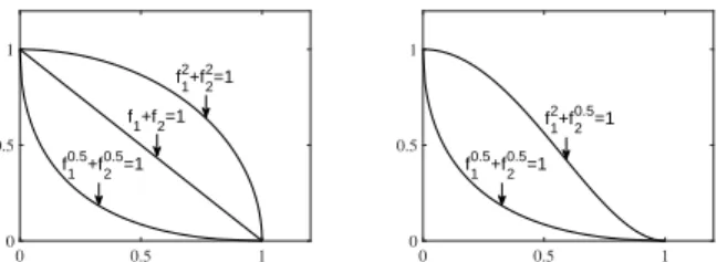
0 0.5 1 0 0.5 1 f 1+f2=1 f 1 0.5+f 2 0.5=1 f 1 2+f 2 2=1 0 0.5 1 0 0.5 1 f 1 0.5+f 2 0.5=1 f 1 2+f 2 0.5=1
Fig. 1. The effectiveness of pi in controlling the shape of the PF
fp1
1 +f
p2
2 = 1, where the PF is convex, concave and linear whenpi<1,
pi>1, andpi= 1, respectively. In addition, the PF is symmetrical or
asymmetrical whenpihave the same or different values, respectively.
intersects all the axes. However, since the PFs of some MOPs do not intersect all the axes (e.g., DTLZ7 [33]), the objective values are translated by subtracting the ideal point to make the PFs consistent with (3) [21]. It is worth noting that in some recent studies [17], [34], the objective values are suggested to be subtracted by a point lower than the ideal point, i.e., fi′ = fi−(z∗i −ϵi) with ϵi >
0. However, according to the experimental results given
in Section V-F, a better performance is achieved in the
proposed GFM whenϵi= 0.
The model in (3) is a generalization of (1) and (2), which has better ability in expressing complicated PF shapes. In contrast to the modes in (1) and (2), which can only approximate symmetrical PFs or linear PFs, the proposed model in (3) can approximate convex,
concave and linear PFs in terms of the i-th objective
when pi < 1, pi > 1, and pi = 1, respectively. In addition, the PFs become symmetrical or asymmetrical
whenpi have the same or different values, respectively.
In addition, while the PF to be modeled by (1) should be well normalized, the proposed model in (3) is capable of modeling PFs with arbitrarily scaled PFs due to the parameters a1, . . . , aM. Fig. 1 depicts five PFs obtained by using the model in (3) with different settings of
p1, . . . , pM, which clearly confirms the effectiveness ofpi in controlling the shape of the estimated PF. As further illustrations to the properties of the model, we have the following two propositions.
Proposition 1: All of the points sampled on the surface generated by (3) are mutually non-dominated.
Proof: Given a point x1 arbitrarily sampled on the
surface generated by (3), for any point x2 which is
dominated byx1, it satisfies: { ∀i∈1, . . . , M : aif pi i (x1)≤aif pi i (x2) ∃j∈1, . . . , M : ajf pj j (x1)< ajf pj j (x2) ,
wherea1, . . . , aM, p1, . . . , pM >0and fi(x1)denotes the
i-th objective value of pointx1. Then we have:
ΣMi=1aif pi
i (x2)>ΣMi=1aif pi
i (x1) = 1.
Therefore,x2 cannot be on the surface generated by (3).
Analogously, for any point x3 which dominates x1, it
satisfies: ΣMi=1aif pi i (x3)<ΣMi=1aif pi i (x1) = 1,
which indicates that x3 cannot be on the surface gener-ated by (3) either. Therefore, all the points on the surface
generated by (3) can neither be dominated by x1 nor
dominate x1, i.e., they are mutually non-dominated.
Proposition 2: The model in (3) satisfies the strictly increasing sufficiency property 2 [35] , i.e., the function
of the model is strictly increasing on each objective.
Proof: Let G = a1f p1 1 +a2f p2 2 +. . . +aMf pM M −1, according to (3), we have ∂G ∂fi =aipifipi−1>0,∀i∈1, . . . , M , where f1, . . . , fM, a1, . . . , aM, p1, . . . , pM >0, hence Gis a strictly increasing function on each objective fi.
The above propositions support that the proposed model in (3) has good capability in providing a com-prehensive outline of the estimated PF shape and thus guides the search process towards promising directions, where more details will be demonstrated in Section IV.
B. The Training Method in GFM
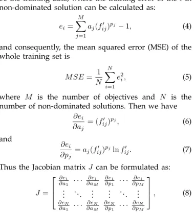
In the proposed GFM, the training process is per-formed by minimizing the error of the model with re-spect to the non-dominated solutions by the Levenberg-Marquardt algorithm [36], which is commonly seen in the training of feedforward neural networks. The reason that we use Levenberg-Marquardt algorithm is due to the fact that it is more efficient than other gradient based techniques in training models with a few parameters [37]. To begin with, a set of non-dominated solutions is collected from the current population and translated to be the training data, where the training error of thei-th non-dominated solution can be calculated as:
ei= M ∑ j=1 aj(fij′ ) pj−1, (4)
and consequently, the mean squared error (MSE) of the whole training set is
M SE= 1 N N ∑ i=1 e2i, (5)
where M is the number of objectives and N is the
number of non-dominated solutions. Then we have
∂ei ∂aj = (fij′ )pj, (6) and ∂ei ∂pj =aj(fij′ ) pjlnf′ ij. (7)
Thus the Jacobian matrix J can be formulated as:
J = ∂e1 ∂a1 · · · ∂e1 ∂aM ∂e1 ∂p1 · · · ∂e1 ∂pM .. . . .. ... ... . .. ... ∂eN ∂a1 · · · ∂eN ∂aM ∂eN ∂p1 · · · ∂eN ∂pM , (8)
2According to the strictly increasing sufficiency, letG(f) :RM →R
be a strictly increasing function on each coordinate, letF={f∈RM |
G(f) = 0}, thenF is an estimated PF.
and the steps for updating the parameters are
∆ =−[JTJ+λdiag(JTJ)]−1JTe, (9) where e = (e1, . . . , eN)T and λ is the damping factor, which is dynamically adjusted during the iterations.
Finally, the parameters aj and pj can be updated as
follows: {
aj =aj+ ∆j pj =pj+ ∆j+M
, (10)
where ∆j denotes the j-th element of vector ∆. The
above procedure will be iterated until the MSE cannot be decreased.
In order to verify the approximation capability of the proposed GFM, we apply it to the estimation of the PF models of several representative MOPs, i.e., DTLZ1, DTLZ2, DTLZ5, DTLZ7 [33], convex DTLZ2 (CDTLZ2) [9], and inverted DTLZ2 (IDTLZ2) [24] with 3 and 10 objectives, respectively. A number of 100 points on the PF of each test instance are sampled as the training set. Table I lists the true PF, the estimated PF and the final MSE on each test instance, where the MSE is calculated using approximately 10000 points sampled on the true PF. For better observation, Fig. 2 shows the modeling results on all the test instances with 3 objectives.
As evidenced by the results in Table I, the proposed GFM is capable of modeling the PFs of all the 12 test in-stances with low estimation errors with regard to the test data sampled on the true PFs, no matter whether the PF is linear (DTLZ1), concave (DTLZ2), convex (CDTLZ2), degenerated (DTLZ5), disconnected (DTLZ7) or even inverted (IDTLZ2). Since the PFs of DTLZ1, DTLZ2, and CDTLZ2 are simple and regular, GFM has obtained the estimated PFs which are almost the same as the true PFs. As for the problems such as DTLZ5, DTLZ7, and IDTLZ2 which have irregular PFs, the estimated PFs are still able to cover the true PFs, although the shapes are not exactly matched. For example, as shown in Fig. 3, although the PF estimated by GFM is different from the true PF of DTLZ7, the estimated PF is still able to very well fit the non-dominated parts of the true PF. As will be demonstrated in the following section, such an estimated PF model can be used to guide the search towards the true PF and meanwhile maintain proper population diversity, which is particularly desirable in the designs of MOEAs.
IV. THEPROPOSEDGFM-MOEA
A. The GFM Based Fitness Function
The GFM based fitness function is the key component in GFM-MOEA, where the fitness of the candidate so-lutions in the same non-dominated front is measured according to the estimated PF modeled by GFM. Specif-ically, the fitness of a candidate solution is measured by two criteria, the convergence criterion and the diversity criterion. As indicated by the Proposition 2 in Section III-A, since the estimated PF is strictly increasing on each objective, the line connecting the objective vector of a
TABLE I
ESTIMATIONRESULTS OFGFMONDTLZ1, DTLZ2, DTLZ5, DTLZ7, CDTLZ2,ANDIDTLZ2WITH3AND10 OBJECTIVES.
Problem M True PF Estimated PF MSE on Test Set
DTLZ1 3 2f1+ 2f2+ 2f3= 1 2f1+ 2f2+ 2f3= 1 1.9e-13 DTLZ2 3 f12+f22+f32= 1 f12+f22+f32= 1 5.5e-15 DTLZ5 3 2f 2 1+f32= 1 f2 1+f22+f32= 1 2.7e-32 f1=f2
DTLZ7 3 f1[1 + sin(3πf1)] +f2[1 + sin(3πf2)] +f3= 6 0.85f14.36+ 0.85f24.36+ 0.5(f3−2.61)0.61= 1 2.9e-3
CDTLZ2 3 f0.5 1 +f20.5+f3= 1 f10.5+f20.5+f3= 1 6.9e-15 IDTLZ2 3 (1−f1)2+ (1−f2)2+ (1−f3)2= 1 0.49f10.48+ 0.49f20.48+ 0.49f30.48= 1 2.1e-4 DTLZ1 10 ∑Mi=12fi= 1 ∑Mi=12fi= 1 5.0e-12 DTLZ2 10 ∑M i=1fi2= 1 ∑M i=1fi2= 1 5.4e-13 DTLZ5 10 fi= ( √
2/2)M−max(i,2)cos(0.5πθ), i < M 0.85f12+ 0.85f22+ 0.84f32+ 0.82f42+ 0.81f52+ 1.1e-30
fM = sin(0.5πθ), i=M 0.81f62+ 0.83f72+ 0.92f82+ 1.13f92+f102 = 1 DTLZ7 10 fM = 2M−∑iM=1−1fi[1 + sin(3πfi)] ∑iM=1−10.13fi1.13+ 0.07(fM−4.76) = 1 4.4e-3 CDTLZ2 10 ∑Mi=1−1fi0.5+fM= 1 ∑Mi=1−1f 0.5 i +fM= 1 1.1e-11 IDTLZ2 10 ∑Mi=1(1−fi)2= 1 ∑Mi=10.11fi0.56= 1 8.3e-4
Fig. 2. The PFs models estimated by GFM on 3-objective DTLZ1, DTLZ2, DTLZ5, DTLZ7, CDTLZ2, and IDTLZ2, where the dots are the data points in the training sets, and the surfaces are the estimated PFs.
candidate solutionxand the ideal pointz∗has one and
only one intersection point y on the estimated PF:
y= (r(f1(x)−z1∗) +z∗1, . . . , r(fM(x)−zM∗ ) +zM∗ ), (11)
where the parameter ris determined by
a1[r(f1(x)−z1∗)]
p1+. . .+a
M[r(fM(x)−z∗M)]
pM = 1. (12)
On the basis of the intersection point y, the
conver-gence criterion of candidate solution x is defined as its
Fig. 3. The true PF and the estimated PF of 3-objective DTLZ7.
distance to the intersection point associated with it:
c(x) =∥y−z∗∥ − ∥f(x)−z∗∥, (13)
where ∥ · ∥ is the L2-norm. The diversity criterion of
candidate solution x is calculated by the distance from
the intersection point to its nearest neighbor:
d(x) =∥y−y′∥, (14)
where y′ denotes the nearest intersection point to y
among all the intersection points of the remaining can-didate solutions in the same non-dominated front.
With the convergence criterionc(x)and the diversity
criterion d(x), the fitness of candidate solution x is
further calculated as:
f itness(x) =θ×c(x) + (1−θ)×d(x), (15)
where 0 < θ < 1 is a predefined penalty parameter.
In this work, θ = 0.2 is adopted in all cases, and the
sensibility analysis ofθ can be found in Section V-E.
B. Procedure of GFM-MOEA
For simplicity, the proposed GFM-MOEA (i.e., the MOEA based on GFM) adopts the same framework as NSGA-II [6], where the only difference is that the crowding distance in NSGA-II has been replaced by the
GFM based fitness functionf itness(x)as introduced in
Algorithm 1:The procedure of GFM-MOEA
Input:N (population size),M (number of objectives)
Output:P (final population) 1 P ←RandomInitialize(N); 2 [a1, . . . , aM, p1, . . . , pM]←1;
3 whiletermination criterion not fulfilleddo
4 ifgmod(fr×G) == 0then
5 Estimate the PF by GFM;
6 P′←SelectN parents via binary tournament
selection according to the non-dominated front and fitness of each candidate solution inP;
7 P ←P∪V ariation(P′); 8 [F1, F2, . . .]←N ondominatedSort(P); 9 k←Minimum value s.t.|F1 ∪ . . .∪Fk|>=N; 10 while|F1 ∪ . . .∪Fk|> N do
11 Delete the candidate solution with the worst
fitness value fromFk using (15);
12 Update the fitness of all the remaining candidate
solutions inFkusing (15);
13 P ←F1
∪
. . .∪Fk; 14 returnP;
The pseudocode of the proposed GFM-MOEA is given in Algorithm 1. To begin with, an initial population
with sizeN is randomly generated, and the parameters
a and p in GFM are initialized to the value of 1. At
each generation, GFM is used to model the approximate PF using the non-dominated solutions in the current population as training data. For the sake of stability and
efficiency, GFM is employed every fr×G generations,
where g denotes the current generation number, G
de-notes the maximum number of generations, and fr is
the parameter controlling the frequency. In this work,
fr = 0.1 is adopted in all cases, and the sensibility analysis offr is given in Section V-E.
Afterwards, the mating selection is performed for
selecting N parents from the current population via
the binary tournament selection. More specifically, two candidate solutions are randomly picked up from the population each time, and the one having a smaller non-dominated front number will be selected as a par-ent. If the two candidate solutions are in the same non-dominated front, the candidate solution with bet-ter (larger) fitness value will be selected as a parent.
After the N parents are selected, the same number of
offsprings are reproduced and merged to the population.
To perform environmental selection, the
non-dominated sorting is first performed to divide the merged population into several non-dominated fronts
F1, F2, . . ., where ENS-SS [5] is employed for MOPs and T-ENS [38] is employed for MaOPs. Then, the candidate solution pwith the worst (least) fitness value is deleted fromFk one by one, whereFk is the last front satisfying |F1
∪
. . .∪Fk| >= N, until |F1
∪
. . .∪Fk| = N is reached. It is worth noting that, since the fitness value of each candidate solution is related to those of the others left in the current population, the fitness values
need to be updated after each pis deleted.
C. Time Complexity of GFM-MOEA
The computational cost mainly results from three op-erations in GFM-MOEA, namely, GFM, non-dominated sorting, and environmental selection. In GFM, the most
time-consuming operation is the calculation of ∆ in
(9). Since the size of J is N ×2M with N denoting
the population size and M denoting the number of
objectives, the calculation of JTJ has a time
complex-ity of O(M2N), and the matrix inversion has a time
complexity of O(M3). Hence, the time complexity of
GFM isO(G′M2(M+N)), whereG′ denotes the number
of iterations of the Levenberg-Marquardt algorithm. By adopting ENS, the time complexity of non-dominated
sorting is O(M N2) in the worst case [39]. In
environ-mental selection, the time complexity for calculating
the fitness of all the candidate solutions is O(M N2)
according to (15), and the time complexity for updating the fitness of remaining solutions isO(N3)for deleting at
mostN candidate solutions. Hence, the time complexity
of environmental selection isO(N2(M +N)).
To summarize, suppose that the total number of
gen-erations is G and the frequency of employing GFM
is fr, the overall time complexity of GFM-MOEA is
O(frGG′M2(M+N)) +O(GM N2) +O(GN2(M+N)) =
O(GN3), with the assumption f
rG′ ≪GandM ≪N. V. EMPIRICALSTUDIES
In this section, we first compare the proposed GFM-MOEA with its three variants to verify the effectiveness of the GFM method in guiding the evolutionary multi-objective optimization process. Then, the performance of GFM-MOEA is assessed by the experimental compar-isons with four popular MOEAs on several benchmark MOPs, and the experimental comparisons with four popular MOEAs on several benchmark MaOPs. Finally,
the sensibility analysis of the parameters θ and fr in
GFM-MOEA is presented, and the influence of the ideal point on the performance of GFM-MOEA is studied. All the experiments are performed on the MATLAB platform for evolutionary multi-objective optimization [40].
A. Experimental Settings
1) Compared MOEAs: Apart from the proposed GFM-MOEA, four classical MOEAs are involved in the exper-iments on MOPs, namely, NSGA-II [6], MOEA/D [8], IBEA [41], and MOEA/D-AWA [17], which belong to Pareto dominance based MOEAs, decomposition based MOEAs, indicator based MOEAs, and decomposition based MOEAs, respectively. In particular, MOEA/D-AWA is a variant of MOEA/D tailored for MOPs with complex PFs. Four recently proposed MOEAs are used in the experiment on MaOPs, namely, MOEA/DD [42], RVEA [21], MOEA/D-PaS [20], and VaEA [43], all of which have been verified to be effective in tackling MaOPs. In MOEA/D, MOEA/D-AWA, MOEA/DD, and
MOEA/D-PaS, the size of neighborhood T is set to
0.9, and the maximum number of solutions replaced by each offspringnr is set to⌈0.01N⌉, withN denoting the population size. In addition, the Tchebycheff approach with transformed reference vectors [44] is utilized as the scalarization approach in MOEA/D. For MOEA/D-AWA, the ratio of updated weight vectors is set to 0.05, the ratio of iterations to evolve with only MOEA/D is set to 0.8, and the generation interval of utilizing AWA is set to 5 for DTLZ1, DTLZ3, IDTLZ1, WFG1, WFG2, IWFG1, IWFG2, and MaF1–MaF15, and 2 for the rest problems. For IBEA, the fitness scaling factor κ is set to 0.05. For
RVEA, the penalty parameter αin APD is set to 2, and
the parameter fr controlling the frequency of reference
vector adaption is set to 0.1. The penalty parameterθand
the frequencyfr of employing GFM in GFM-MOEA are
set to 0.2 and 0.1, respectively.
2) Test problems:43 widely used multi-objective bench-mark problems are used as the test problems, i.e., ZDT1–ZDT4, ZDT6 [45], DTLZ1–DTLZ7 [33], convex DTLZ2 (CDTLZ2) [9], inverted DTLZ1–DTLZ2 (IDTLZ1– IDTLZ2) [24], WFG1–WFG9 [46], inverted WFG1–WFG4 (IWFG1–IWFG4), and MaF1–MaF15 [16]. Note that the IWFG1–IWFG4 are designed by a similar method to IDTLZ1 [24]. The length of decision variables of ZDT1– ZDT3 is set to 30, and the length of decision variables of ZDT4 and ZDT6 is set to 10. For all the DTLZ problems,
the length of decision variables is set to K +M −1,
where M denotes the number of objectives, and K is
set to 5 for DTLZ1 and IDTLZ1, 20 for DTLZ7, and 10 for the others. As for all the WFG problems, the length
of decision variables is set to K+L, where K and L
are set to M −1 and 10 respectively. The lengths of
decision variables for the MaF problems are referred to [16]. The maximum number of generations is adopted as the termination criterion for all compared MOEAs, which is set to 500 for DTLZ1, DTLZ3, IDTLZ1, WFG1, WFG2, IWFG1, IWFG2, and MaF1–MaF15, and 200 for all the other problems.
3) Population sizing:The population size of all the com-pared MOEAs is set to the same on each MOP, namely, 100, 105, 126 and 275 for 2-, 3-, 5- and 10-objective MOPs, respectively. Accordingly, in MOEA/D, MOEA/D-AWA, MOEA/DD, RVEA, and MOEA/D-PaS, the parameters
(p1, p2)controlling the number of reference vectors along the outer and inner layers [9] are set to (99,0), (13,0),
(5,0) and (3,2) for 2, 3, 5 and 10 objectives, since the number of reference vectors needs to be consistent with the population size in these algorithms.
4) Genetic operators: The simulated binary crossover (SBX) [47] and polynomial mutation [48] are employed in all the compared MOEAs for creating offsprings, and the parameter settings of them are identical in all the MOEAs for fair comparison. To be specific, the probabil-ity of crossover is set to 1, the probabilprobabil-ity of mutation is
set to 1/D, and the distribution index of both SBX and
polynomial mutation is set to 20, where D denotes the
length of decision variables.
5) Performance metrics: The inverted generational
dis-tance (IGD) [49] and hypervolume (HV) [10] are em-ployed to assess the performance of the compared MOEAs, both of which can measure the convergence and diversity of the results simultaneously. A smaller value of IGD indicates a better quality of the result, while a larger value of HV signals a better quality. In the calculation of IGD, roughly 10000 points uniformly sampled on the true PF of each test instance are adopted as the reference points. The detailed sampling method for each test instance can be found in [50]. As for the calculation of HV, the reference point is set to(1, . . . ,1), and the objective values are normalized by the point
1.1×znad before the calculation, where znad denotes
the nadir point of the true PF. All the experiments are performed for 30 runs independently, and the mean value and the standard deviation of each result are recorded. Furthermore, the results are also analyzed by the Wilcoxon rank sum test with a significance level of 0.05, where ’+’, ’−’ and ’≈’ indicate that the result of other MOEA is significantly better, significantly worse and statistically similar to that of the proposed GFM-MOEA, respectively.
B. Effectiveness of GFM
To verify whether GFM is able to enhance the per-formance consistency of MOEAs in solving MOPs with different types of PFs, GFM-MOEA is compared with three of its variants, in which the parametersaandpare fixed to several specific values instead of being learned in the training of GFM. The DTLZ2 and CDTLZ2 are used as the test problems in the experiment, where DTLZ2 has a concave PF and CDTLZ2 has a convex PF.
For the first variant of GFM-MOEA, we make its
parametersaandpidentical with those in the true PF of
DTLZ2, i.e.,a1=. . .=aM = 1andp1=. . .=pM = 2, as shown in Table I. Analogically, we make the parameters
aandpof the second variant identical with those in the
true PF of CDTLZ2, wherea1=. . .=aM = 1,p1=. . .=
pM−1= 0.5andpM = 1. As for the third variant, we set a1=. . .=aM = 1andp1=. . .=pM = 1. For simplicity, the three variants of GFM-MOEA are hereafter denoted
as GFM-MOEADT LZ2, GFM-MOEACDT LZ2, and
GFM-MOEA1, respectively.
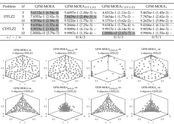
The statistical results of HV values of GFM-MOEA and its three variants on DTLZ2 and CDTLZ2 are given in Table II, and the non-dominated solution sets with the median HV obtained by the four MOEAs on the prob-lems with 3 objectives are plotted in Fig. 4. From Table II and Fig. 4, the following observations can be obtained. First, GFM-MOEA achieves a competitive performance on both DTLZ2 and CDTLZ2 in comparison with the three variants, which indicates the effectiveness of the proposed GFM in capturing different PF geometries. The GFM-MOEA demonstrates a similar performance with
GFM-MOEADT LZ2 on DTLZ2, and similar performance
with GFM-MOEACDT LZ2 on CDTLZ2. Secondly, since
TABLE II
STATISTICALRESULTS OFHV VALUESOBTAINED BYGFM-MOEAAND ITSTHREEVARIANTS ONDTLZ2ANDCDTLZ2WITH3, 5AND10
OBJECTIVES.
Problem M GFM-MOEA GFM-MOEADT LZ2 GFM-MOEACDT LZ2 GFM-MOEA1 DTLZ2
3 5.6112e-1 (6.54e-4) 5.6097e-1 (1.00e-3)≈ 4.8312e-1 (1.11e-2)− 5.4676e-1 (1.45e-3)− 5 7.8353e-1 (2.92e-3) 7.8429e-1 (2.49e-3)≈ 7.0634e-1 (1.77e-2)− 7.7874e-1 (2.82e-3)− 10 9.5536e-1 (2.39e-3) 9.5220e-1 (1.75e-3)− 9.1751e-1 (3.62e-2)− 9.2625e-1 (5.89e-2)≈ CDTLZ2
3 9.6354e-1 (1.57e-4) 9.2666e-1 (7.25e-3)− 9.6343e-1 (1.75e-4)≈ 9.4166e-1 (6.11e-3)−
5 9.9919e-1 (3.92e-5) 9.9089e-1 (4.11e-3)− 9.9917e-1 (4.14e-5)≈ 9.9018e-1 (1.46e-3)−
10 1.0000e+0 (5.79e-7) 9.9987e-1 (1.35e-4)− 1.0000e+0 (2.67e-7)≈ 9.9969e-1 (1.55e-4)−
+/−/≈ 0/4/2 0/3/3 0/5/1 0 0 0 0.5 GFM-MOEA on 3-objective DTLZ2 0.5 0.5 1 1 1 0 0 0 0.5 GFM-MOEADTLZ2 on 3-objective DTLZ2 0.5 0.5 1 1 1 0 0 0 0.5 GFM-MOEACDTLZ2 on 3-objective DTLZ2 0.5 0.5 1 1 1 0 0 0 0.5 GFM-MOEA1 on 3-objective DTLZ2 0.5 0.5 1 1 1 0 0 0 0.5 GFM-MOEA on 3-objective CDTLZ2 0.5 0.5 1 1 1 0 0 0 0.5 GFM-MOEADTLZ2 on 3-objective CDTLZ2 0.5 0.5 1 1 1 0 0 0 0.5 GFM-MOEACDTLZ2 on 3-objective CDTLZ2 0.5 0.5 1 1 1 0 0 0 0.5 GFM-MOEA1 on 3-objective CDTLZ2 0.5 0.5 1 1 1
Fig. 4. The non-dominated solution set with the median HV among 30 runs obtained by GFM-MOEA and its three variants on DTLZ2 and CDTLZ2 with 3 objectives.
identical with the true PF of DTLZ2, GFM-MOEADT LZ2
can obtain similar HV values with the proposed GFM-MOEA on DTLZ2. However, its performance consid-erably deteriorates when meeting CDTLZ2, since the model is concave but the true PF of CDTLZ2 is con-vex. Due to the same reason, the performance of GFM-MOEACDT LZ2 is as good as GFM-MOEA on CDTLZ2,
but GFM-MOEACDT LZ2 obtains a non-dominated
solu-tion set with poor diversity on DTLZ2. Thirdly, for
GFM-MOEA1 which adopts a linear front model, its
perfor-mance is not satisfactory on either DTLZ2 or CDTLZ2. This is mainly due to the fact that the linear front model is identical with neither DTLZ2 nor CDTLZ2.
In summary, the proposed GFM can adaptively esti-mate the PF models of different geometries, such that GFM-MOEA performs consistently in approximating the PFs of both DTLZ2 and CDTLZ2. By contrast, a constant model setting cannot make GFM-MOEA work well on MOPs with various PFs. This confirms that the proposed GFM is crucial to the performance of GFM-MOEA.
In order to further assess the accuracy of the proposed GFM method during the optimization procedure, we record the MSE values returned by GFM with respect to 10000 points sampled on the true PF of 3-objective DTLZ1, DTLZ2, DTLZ5, DTLZ7, CDTLZ2, and IDTLZ2, averaging over 30 runs. As shown in Fig. 5, the MSE values are gradually decreased as the number of gener-ations increase, which indicates promising convergence
0 0.2 0.4 0.6 0.8 1 Ratio of Generations 10-10 10-5 100 105 MSE 3 objectives DTLZ1 DTLZ2 DTLZ5 DTLZ7 CDTLZ2 IDTLZ2
Fig. 5. MSE values returned by GFM during the optimization proce-dure of GFM-MOEA on 3-objective DTLZ1, DTLZ2, DTLZ5, DTLZ7, CDTLZ2, and IDTLZ2, with respect to 10000 points sampled on each true PF, averaging over 30 runs.
of GFM. In addition, as shown in Fig. 6, the similarity be-tween the estimated PF and the true PF of DTLZ1 is also substantially increased with respect to the number of generations. Such observations have further confirmed the accuracy of the proposed GFM method.
C. Performance on MOPs
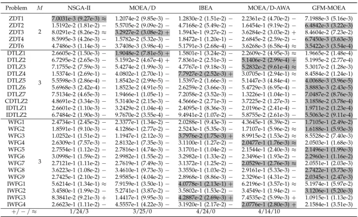
The experimental results of GFM-MOEA, NSGA-II, MOEA/D, IBEA, and MOEA/D-AWA on 2-objective ZDT1–ZDT4 and ZDT6, and 3-objective DTLZ1–DTLZ7, CDTLZ2, IDTLZ1, IDTLZ2, WFG1–WFG9, and IWFG1– IWFG4 are listed in Table III. According to the
statisti-TABLE III
STATISTICALRESULTS OFIGD VALUESOBTAINED BYNSGA-II, MOEA/D, IBEA, MOEA/D-AWA,ANDGFM-MOEAON2-OBJECTIVE
ZDT1–ZDT4ANDZDT6,AND3-OBJECTIVEDTLZ1–DTLZ7, CDTLZ2, IDTLZ1, IDTLZ2, WFG1–WFG9,ANDIWFG1–IWFG4.
Problem M NSGA-II MOEA/D IBEA MOEA/D-AWA GFM-MOEA
ZDT1 2
7.0031e-3 (9.27e-3)≈ 1.2074e-2 (9.85e-3)− 1.2830e-2 (1.51e-2)− 2.2361e-2 (4.70e-2)− 7.1988e-3 (5.16e-3) ZDT2 1.5192e-2 (1.81e-2)− 5.5705e-2 (9.09e-2)− 4.7168e-2 (5.49e-2)− 1.6454e-1 (9.19e-2)− 6.4842e-3 (3.22e-3) ZDT3 8.0291e-2 (8.26e-2)≈ 3.2927e-2 (3.08e-2)+ 1.5943e-1 (9.27e-2)− 3.6284e-2 (3.03e-2)+ 8.4604e-2 (7.23e-2) ZDT4 8.5995e-3 (4.26e-3)− 1.5782e-2 (5.32e-3)− 1.8472e-1 (1.20e-1)− 2.6845e-2 (2.59e-2)− 6.7450e-3 (3.63e-3) ZDT6 4.7486e-3 (1.14e-3)− 3.7408e-3 (3.98e-4)− 5.1791e-3 (2.68e-4)− 3.6268e-3 (6.58e-4)≈ 3.5422e-3 (3.54e-4) DTLZ1
3
2.6605e-2 (1.50e-3)− 1.9048e-2 (7.81e-5)+ 1.5801e-1 (3.24e-2)− 2.2609e-2 (4.95e-3)≈ 1.9665e-2 (1.48e-4) DTLZ2 6.7295e-2 (2.65e-3)− 5.1592e-2 (4.67e-4)+ 7.8361e-2 (2.51e-3)− 5.1406e-2 (2.99e-4)+ 5.1995e-2 (2.77e-4) DTLZ3 7.1755e-2 (7.59e-3)− 5.4274e-2 (1.99e-3)− 4.7767e-1 (9.18e-3)− 5.2832e-2 (9.61e-4)≈ 5.3017e-2 (1.28e-3) DTLZ4 1.5374e-1 (2.69e-1)− 4.0802e-1 (2.70e-1)− 7.7927e-2 (2.52e-3)+ 3.0705e-1 (2.94e-1)≈ 8.4584e-2 (1.24e-1) DTLZ5 5.5598e-3 (2.86e-4)− 1.8542e-2 (2.99e-5)− 1.5397e-2 (1.66e-3)− 5.1447e-3 (4.84e-4)− 4.0068e-3 (3.96e-5) DTLZ6 5.6968e-3 (2.42e-4)− 1.8523e-2 (4.91e-5)− 2.6259e-2 (3.66e-3)− 5.4729e-3 (6.95e-4)− 3.8883e-3 (2.43e-5) DTLZ7 7.5134e-2 (4.65e-3)− 1.9466e-1 (1.05e-1)− 7.2058e-2 (3.52e-3)− 1.3226e-1 (1.04e-1)− 7.0487e-2 (8.76e-3) CDTLZ2 4.8691e-2 (3.34e-3)− 5.3140e-2 (2.15e-3)− 4.5666e-2 (2.71e-3)− 3.7225e-2 (1.27e-3)− 3.1858e-2 (3.78e-4) IDTLZ1 2.6601e-2 (1.10e-3)− 3.2429e-2 (1.04e-4)− 2.4095e-1 (8.36e-3)− 2.0196e-2 (2.41e-4)− 1.9711e-2 (1.23e-4) IDTLZ2 6.7484e-2 (1.90e-3)− 9.7670e-2 (3.55e-4)− 9.4941e-2 (1.07e-2)− 5.8755e-2 (2.61e-3)− 5.5063e-2 (9.11e-4)
WFG1
3
2.4734e-1 (2.45e-2)− 2.3377e-1 (1.34e-2)− 2.0288e-1 (9.43e-3)− 4.3645e-1 (8.39e-2)− 1.7105e-1 (2.49e-2) WFG2 1.8591e-1 (9.10e-3)− 4.1286e-1 (2.77e-2)− 2.5243e-1 (5.35e-3)− 1.7107e-1 (5.96e-2)≈ 1.6188e-1 (5.93e-3) WFG3 1.0252e-1 (1.51e-2)− 1.1947e-1 (2.12e-3)− 3.7976e-2 (1.75e-3)+ 8.9915e-2 (1.53e-2)≈ 8.5528e-2 (7.40e-3) WFG4 2.6309e-1 (7.57e-3)− 2.8132e-1 (7.35e-3)− 3.1100e-1 (1.27e-2)− 2.0477e-1 (1.76e-3)≈ 2.0503e-1 (1.68e-3) WFG5 2.7554e-1 (1.12e-2)− 2.7816e-1 (4.74e-3)− 3.1701e-1 (1.04e-2)− 2.1544e-1 (2.40e-3)≈ 2.1496e-1 (1.99e-3) WFG6 3.0998e-1 (1.59e-2)− 2.9982e-1 (1.55e-2)− 3.2982e-1 (1.33e-2)− 2.3496e-1 (1.93e-2)− 2.2960e-1 (1.16e-2) WFG7 2.7121e-1 (1.11e-2)− 2.7619e-1 (7.49e-3)− 3.1372e-1 (1.25e-2)− 2.0529e-1 (2.76e-3)≈ 2.0551e-1 (2.03e-3) WFG8 3.6223e-1 (1.08e-2)− 3.4610e-1 (9.73e-3)− 3.3550e-1 (1.03e-2)− 2.9161e-1 (5.33e-3)− 2.7422e-1 (3.73e-3) WFG9 2.7425e-1 (2.10e-2)− 2.9585e-1 (4.04e-2)− 2.8968e-1 (8.86e-3)− 2.3296e-1 (4.31e-2)− 2.0345e-1 (2.47e-3) IWFG1 5.6214e-1 (1.34e-1)≈ 7.9159e-1 (3.50e-1)− 4.0778e-1 (2.13e-1)+ 6.2196e-1 (3.57e-1)≈ 5.1974e-1 (5.97e-2) IWFG2 3.4580e-1 (1.99e-2)− 5.2741e-1 (3.87e-2)− 3.5802e-1 (1.53e-2)− 3.4549e-1 (1.94e-2)− 3.1206e-1 (5.20e-3) IWFG3 8.3841e-2 (9.21e-3)+ 1.4417e-1 (9.95e-3)− 4.2887e-2 (2.69e-3)+ 7.4535e-2 (5.99e-3)+ 1.0915e-1 (1.13e-2) IWFG4 2.6623e-1 (1.11e-2)− 4.5557e-1 (4.22e-3)− 3.1920e-1 (2.17e-2)− 2.0776e-1 (2.80e-3)+ 2.1584e-1 (3.51e-3)
+/−/≈ 1/24/3 3/25/0 4/24/0 4/14/10
cal results in terms of IGD metric, NSGA-II performs the best on ZDT1, MOEA/D performs the best on ZDT3 and DTLZ1, IBEA outperforms the other com-pared algorithms on DTLZ4, WFG3, IWFG1, and IWFG3, MOEA/D-AWA performs better than the compared al-gorithms on DTLZ2, DTLZ3, WFG4, WFG7, and IWFG4, and GFM-MOEA gains the best results on all the remain-ing 16 MOPs. In conclusion, GFM-MOEA is competitive to the four compared MOEAs on MOPs with simple PFs (ZDT1, ZDT2, ZDT4, ZDT6, DTLZ1–DTLZ4, and CDTLZ2), while it performs remarkably better than them on MOPs with complex PFs (DTLZ5–DTLZ7, IDTLZ1, and IDTLZ2) and scaled PFs (WFG1, WFG2, WFG5, WFG6, WFG8, WFG9, and IWFG2).
Fig. 7 shows the non-dominated solution set with the median IGD obtained by the five compared MOEAs on DTLZ2, CDTLZ2, and IWFG4. For NSGA-II, it first sorts the solutions based on their Pareto dominance relations, and then distinguishes the solutions in the same front by crowding distance. However, it seems that the crowding distance is not very effective in diversity preservation of NSGA-II on MOPs, since the distribution of the solutions obtained by NSGA-II is satisfactory on none of the three MOPs as shown in Fig. 7.
As for MOEA/D, it makes each solution converge to the same direction with one of the predefined uniformly distributed weight vectors, thus the final population can hold the same uniformity with the weight vectors. As shown in the second column of Fig. 7, the solutions
obtained by MOEA/D have a good distribution on DTLZ2, except that the solutions located on the border are slightly more crowded than those located in the mid-dle. This should be attributed to the reason mentioned in Section I, where the weight vectors are uniformly distributed on a hyperplane, hence the solutions on the border will be more crowded than those in the middle when they are mapped to a concave surface. This phenomenon becomes worse on CDTLZ2, where almost all the solutions obtained by MOEA/D are located in the middle of the PF. For IWFG4, however, since the predefined weight vectors can only cover part of the inverted PF, MOEA/D is unable to make all the solutions distribute uniformly on the PF.
IBEA is an indicator based MOEA, where the selection criterion is defined on the basis of a binary indicator. According to the solutions obtained by IBEA shown in Fig. 7, the indicator employed by IBEA is easily biased, which makes the solutions distributed in the middle of the PFs of DTLZ2, CDTLZ2 and IWFG4. Regarding the variant of MOEA/D tailored for solving MOPs with complex PFs, MOEA/D-AWA, it obtains an obviously better distribution of solutions than MOEA/D on MOPs with complex PFs. In contrast to the above four MOEAs, by measuring the solutions according to the PF estimated by GFM, the solutions obtained by GFM-MOEA distribute well on all of the three MOPs, no matter whether the true PF is concave, convex or inverted. Therefore, GFM-MOEA has better performance
0 0 0 0.5 NSGA-II on 3-objective DTLZ2 0.5 0.5 1 1 1 0 0 0 0.5 MOEA/D on 3-objective DTLZ2 0.5 0.5 1 1 1 0 0 0 0.5 IBEA on 3-objective DTLZ2 0.5 0.5 1 1 1 0 0 0 0.5 MOEA/D-AWA on 3-objective DTLZ2 0.5 0.5 1 1 1 0 0 0 0.5 GFM-MOEA on 3-objective DTLZ2 0.5 0.5 1 1 1 0 0 0 0.5 NSGA-II on 3-objective CDTLZ2 0.5 0.5 1 1 1 0 0 0 0.5 MOEA/D on 3-objective CDTLZ2 0.5 0.5 1 1 1 0 0 0 0.5 IBEA on 3-objective CDTLZ2 0.5 0.5 1 1 1 0 0 0 0.5 MOEA/D-AWA on 3-objective CDTLZ2 0.5 0.5 1 1 1 0 0 0 0.5 GFM-MOEA on 3-objective CDTLZ2 0.5 0.5 1 1 1 0 4 2 3 NSGA-II on 3-objective IWFG4 4 5 6 6 6 0 4 2 3 MOEA/D on 3-objective IWFG4 5 4 6 6 6 0 4 2 3 IBEA on 3-objective IWFG4 4 5 6 6 6 0 2 4 3 MOEA/D-AWA on 3-objective IWFG4 4 5 6 6 6 0 4 2 3 GFM-MOEA on 3-objective IWFG4 4 5 6 6 6
Fig. 7. The non-dominated solution set with the median IGD among 30 runs obtained by NSGA-II, MOEA/D, IBEA, MOEA/D-AWA, and GFM-MOEA on DTLZ2, CDTLZ2, and IDTLZ2 with 3 objectives.
Fig. 6. Estimated PFs obtained at different generations of GFM-MOEA on 3-objective DLTZ1, where the non-dominated solutions are shown in solid points, and the estimated PFs are shown in surfaces.
consistency in solving MOPs with different types of PFs in comparison with existing MOEAs.
D. Perfromance on MaOPs
In this subsection, the proposed GFM-MOEA is com-pared with MOEA/DD, RVEA, MOEA/D-PaS, and
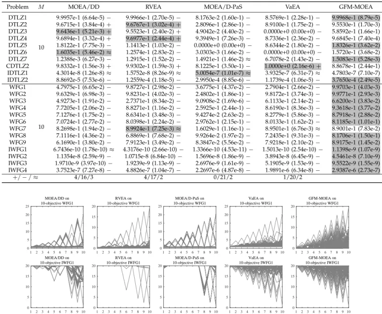
VaEA for solving MaOPs. The HV values of the four compared MOEAs on 10-objective DTLZ and WFG prob-lems are listed in Table IV. As shown in the table, GFM-MOEA performs the best on 16 of the 23 test instances in terms of HV, while the numbers of best results obtained by MOEA/DD, RVEA, MOEA/D-PaS, and VaEA are 2, 3, 1 and 1, respectively. In terms of the Wilcoxon rank sum test, the proportion of test instances where GFM-MOEA performs significantly better than GFM-MOEA/DD, RVEA, MOEA/D-PaS, and VaEA is 16/23, 17/23, 21/23 and 20/23, respectively.
For visual observations of the differences between the results, Fig. 8 plots the non-dominated solution sets with the median HV values among 30 runs obtained by the five MOEAs on WFG1 and IWFG1. It is clear that VaEA and GFM-MOEA can find a set of solutions covering the whole PF of IWFG1, while only GFM-MOEA can exhibit a good diversity performance on WFG1. As a result, GFM-MOEA is also able to perform consistently on MaOPs with different types of PFs.
The statistical results of MOEA/DD, RVEA,
MOEA/D-PaS, VaEA, and GFM-MOEA on 2-objective ZDT problems and 3-objective DTLZ and WFG problems can be found in Supplementary Materials I. In order to verify the performance of these MOEAs on more challenging MaOPs, they are tested on MaF1–MaF15, which are designed for IEEE CEC’2018 Competition on Evolutionary Many-Objective Optimization and contain diverse and complicated PFs. The corresponding results can be found in Supplementary Materials II. The non-dominated solution set with median performance obtained by all the 9 compared MOEAs on all the test instances can be found in Supplementary Materials
TABLE IV
STATISTICALRESULTS OFHV VALUESOBTAINED BYMOEA/DD, RVEA, MOEA/D-PAS, VAEA,ANDGFM-MOEAONDTLZ1–DTLZ7,
CDTLZ2, IDTLZ1, IDTLZ2, WFG1–WFG9,ANDIWFG1–IWFG4WITH10 OBJECTIVES.
Problem M MOEA/DD RVEA MOEA/D-PaS VaEA GFM-MOEA
DTLZ1
10
9.9957e-1 (6.64e-5)− 9.9966e-1 (2.70e-5)− 8.1763e-2 (1.60e-1)− 8.5769e-1 (2.28e-1)− 9.9968e-1 (8.79e-5) DTLZ2 9.6715e-1 (3.84e-4)+ 9.6767e-1 (3.02e-4)+ 2.8096e-1 (2.86e-1)− 8.9100e-1 (1.75e-2)− 9.5530e-1 (1.70e-3) DTLZ3 9.6436e-1 (5.21e-3)+ 9.5523e-1 (2.40e-2)+ 4.9042e-2 (4.40e-2)− 0.0000e+0 (0.00e+0)− 5.8592e-1 (1.66e-1) DTLZ4 9.6894e-1 (3.32e-4)+ 9.6977e-1 (2.44e-4)+ 9.3949e-1 (7.26e-3)− 8.7336e-1 (2.36e-2)− 9.6845e-1 (7.40e-4) DTLZ5 1.8122e-1 (7.75e-3)− 1.1413e-1 (1.03e-2)− 0.0000e+0 (0.00e+0)− 8.6344e-2 (1.80e-2)− 1.8326e-1 (3.62e-2) DTLZ6 1.6035e-1 (5.46e-2)≈ 1.2574e-1 (2.83e-2)− 3.0303e-3 (1.66e-2)− 0.0000e+0 (0.00e+0)− 1.5720e-1 (3.68e-2) DTLZ7 1.2388e-3 (6.27e-3)− 1.2915e-1 (1.52e-2)− 1.4921e-1 (1.46e-2)≈ 6.7078e-2 (1.43e-2)− 1.5083e-1 (5.28e-3) CDTLZ2 9.8332e-1 (1.56e-3)+ 9.9302e-1 (1.59e-3)+ 8.1225e-1 (3.50e-1)− 1.0000e+0 (2.16e-6)+ 8.8678e-1 (2.44e-1) IDTLZ1 4.3014e-8 (1.26e-8)≈ 1.5752e-8 (8.26e-9)≈ 5.0054e-7 (1.01e-7)≈ 3.9325e-7 (6.31e-7)≈ 4.7803e-7 (7.10e-7) IDTLZ2 8.8692e-5 (7.53e-6)− 1.2559e-4 (1.18e-5)− 2.9950e-4 (8.85e-6)− 1.1739e-4 (1.06e-5)− 3.7650e-4 (2.49e-5)
WFG1
10
4.7975e-1 (6.65e-2)− 9.8727e-1 (2.98e-2)− 3.6775e-1 (4.37e-2)− 2.7904e-1 (2.66e-2)− 9.9703e-1 (4.03e-3) WFG2 9.6329e-1 (6.98e-3)− 9.8231e-1 (4.02e-3)− 2.4802e-1 (1.86e-1)− 9.8172e-1 (3.74e-3)− 9.9771e-1 (2.93e-3) WFG3 4.9273e-1 (1.91e-2)− 2.7371e-1 (8.34e-2)− 9.0908e-2 (1.69e-6)− 6.1133e-1 (2.14e-2)− 6.6200e-1 (3.83e-2) WFG4 7.7205e-1 (2.06e-2)− 8.8271e-1 (1.16e-2)− 2.5925e-1 (2.44e-1)− 8.6190e-1 (8.36e-3)− 9.3618e-1 (3.77e-2) WFG5 7.1276e-1 (1.75e-2)− 8.6341e-1 (3.48e-3)− 9.4274e-2 (2.63e-2)− 8.2779e-1 (5.86e-3)− 8.7918e-1 (2.88e-2) WFG6 7.0724e-1 (2.77e-2)− 8.0398e-1 (2.24e-2)− 2.9762e-1 (2.15e-1)− 8.0133e-1 (1.62e-2)− 8.1185e-1 (1.01e-1) WFG7 8.2698e-1 (1.94e-2)− 8.9924e-1 (7.25e-3)≈ 1.6029e-1 (1.16e-1)− 8.9501e-1 (6.76e-3)≈ 8.9001e-1 (7.83e-2) WFG8 7.1116e-1 (4.36e-2)− 6.8869e-1 (7.68e-2)− 9.9264e-2 (1.97e-2)− 7.2435e-1 (9.31e-3)− 8.1706e-1 (1.50e-1) WFG9 6.1690e-1 (3.80e-2)− 7.9123e-1 (3.49e-2)− 8.3847e-2 (5.56e-2)− 7.9218e-1 (2.10e-2)− 8.9175e-1 (1.45e-2) IWFG1 6.7436e-10 (1.78e-10)≈ 4.3176e-10 (2.66e-10)− 1.3366e-10 (4.53e-11)− 1.5013e-10 (2.54e-10)− 1.1398e-9 (1.07e-9) IWFG2 1.1354e-8 (2.59e-9)− 1.0715e-8 (6.84e-10)− 1.5696e-8 (1.86e-9)− 3.8943e-8 (6.45e-9)− 4.5461e-8 (7.10e-9) IWFG3 1.9710e-9 (3.97e-10)− 1.9239e-9 (1.13e-9)− 2.6976e-9 (1.61e-9)− 5.1905e-9 (1.53e-9)− 9.5522e-9 (1.55e-9) IWFG4 3.7523e-7 (7.27e-8)− 4.8826e-7 (1.04e-7)− 2.2697e-6 (4.87e-8)− 1.9891e-6 (6.34e-8)− 2.9387e-6 (2.73e-7)
+/−/≈ 4/16/3 4/17/2 0/21/2 1/20/2 1 2 3 4 5 6 7 8 9 10 0 5 10 15 20 25 MOEA/DD on 10-objective WFG1 1 2 3 4 5 6 7 8 9 10 0 5 10 15 20 RVEA on 10-objective WFG1 1 2 3 4 5 6 7 8 9 10 0 5 10 15 20 25 MOEA/D-PaS on 10-objective WFG1 1 2 3 4 5 6 7 8 9 10 0 5 10 15 20 25 VaEA on 10-objective WFG1 1 2 3 4 5 6 7 8 9 10 0 5 10 15 20 GFM-MOEA on 10-objective WFG1 1 2 3 4 5 6 7 8 9 10 0 5 10 15 20 MOEA/DD on 10-objective IWFG1 1 2 3 4 5 6 7 8 9 10 0 5 10 15 20 RVEA on 10-objective IWFG1 1 2 3 4 5 6 7 8 9 10 0 5 10 15 20 MOEA/D-PaS on 10-objective IWFG1 1 2 3 4 5 6 7 8 9 10 0 5 10 15 20 VaEA on 10-objective IWFG1 1 2 3 4 5 6 7 8 9 10 0 5 10 15 20 GFM-MOEA on 10-objective IWFG1
Fig. 8. The non-dominated solution set with the median HV among 30 runs obtained by MOEA/DD, RVEA, MOEA/D-PaS, VaEA, and GFM-MOEA on WFG1 and IWFG1 with 10 objectives.
III. Furthermore, the comparison between GFM-MOEA and more state-of-the-art MOEAs can be found in Supplementary Materials IV.
E. Parameter Sensitivity Analysis
There are two parameters which need to be set in
GFM-MOEA, i.e., the penalty parameter θ and the
fre-quencyfr. Here, we investigate the influence of the two parameters on the performance of GFM-MOEA.
Fig. 9 shows the average HV values of GFM-MOEA on DTLZ1, DTLZ2, DTLZ5, DTLZ7, CDTLZ2, and IDTLZ2 with 3 and 10 objectives over 30 runs, where the pa-rameter θis varied from 0 to 1 and fr is fixed to 0.1. It can be seen from the figure that the HV value rapidly
decreases when θ varies from 0.4 to 1, and it increases
on MOPs with 10 objectives when θ varies from 0 to
0 0.2 0.4 0.6 0.8 1 0 0.2 0.4 0.6 0.8 1 HV 3-objective DTLZ1 DTLZ2 DTLZ5 DTLZ7 CDTLZ2 IDTLZ2 0 0.2 0.4 0.6 0.8 1 0 0.2 0.4 0.6 0.8 1 HV 10-objective DTLZ1 DTLZ2 DTLZ5 DTLZ7 CDTLZ2 IDTLZ2
Fig. 9. The average HV values of GFM-MOEA on DTLZ1, DTLZ2, DTLZ5, DTLZ7, CDTLZ2, and IDTLZ2 with 3 and 10 objectives over 30 runs, whereθis varied from 0 to 1 andfris fixed to 0.1.
0.2. As a result, θ = 0.2 is recommended for consistent
performance.
Fig. 10 shows the average HV values of GFM-MOEA
0 0.1 0.2 0.3 0.4 0.5 fr 0 0.2 0.4 0.6 0.8 1 HV 3-objective DTLZ1 DTLZ2 DTLZ5 DTLZ7 CDTLZ2 IDTLZ2 0 0.1 0.2 0.3 0.4 0.5 fr 0 0.2 0.4 0.6 0.8 1 HV 10-objective DTLZ1 DTLZ2 DTLZ5 DTLZ7 CDTLZ2 IDTLZ2
Fig. 10. The average HV values of GFM-MOEA on DTLZ1, DTLZ2, DTLZ5, DTLZ7, CDTLZ2, and IDTLZ2 with 3 and 10 objectives over 30 runs, whereθis fixed to 0.2 andfris varied from 0 to 0.5.
varied from 0 to 0.5 andθis fixed to 0.2. Note thatfr= 0 indicates that GFM is performed at each generation, and
fr= 0.5implies that GFM is performed only once in one run. It turns out that the HV value decreases on some test instances when fris larger than 0.3. Therefore, fr needs to be set to a relatively small value. By considering the balance between efficiency and effectiveness, fr= 0.1is suggested in all cases.
In summary, it can be concluded from the above observations that the performance of GFM-MOEA is insensitive to the settings of θ and fr, as long as that
fr is smaller than 0.3 andθ is between 0.2 and 0.4.
F. Influence of the Ideal Point
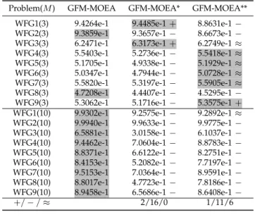
As mentioned in Section III-A, in order to make the PF of the MOP to be solved consistent with the model in GFM, the objective values are translated according to the current ideal point before training the model, i.e., fi′ = fi−zi∗. However, some recent studies [17], [34] pointed out that a point lower than the current ideal point can lead to better performance, i.e., fi′ =fi−(z∗i −ϵi) with ϵi >0. To investigate the effect of the usage of the current ideal point, we follow the settings in [34] to compare GFM-MOEA with two of its variants GFM-MOEA* and
GFM-MOEA**, where ϵi is set to 1 and linearly varied
from 1 to 0 during the optimization process, respectively. Table V lists the average HV values obtained by the three MOEAs on WFG1–WFG9 with 3 and 10 objectives over 30 runs. The statistical results show the superiority of the original GFM-MOEA over the two variants, hence it can be confirmed that the original current ideal point
(i.e., ϵi = 0) is the best for GFM-MOEA. This is due to
the fact that a point lower than the current ideal point can increase the estimation error of GFM, thus leading to a poor performance of the proposed GFM-MOEA. As evidenced by the results in Table VI, the MSE values returned by GFM in the final generation of GFM-MOEA are significantly smaller than those in GFM-MOEA* and GFM-MOEA** on most test instances.
VI. CONCLUSIONS
In this paper, we have proposed a generic front mod-eling (GFM) method for enhancing the performance consistency of MOEAs in tackling MOPs and MaOPs with various PFs. By using the non-dominated solutions
TABLE V
STATISTICALRESULTS OFHV VALUESOBTAINED BYGFM-MOEA
(ϵ= 0), GFM-MOEA* (ϵ= 1),ANDGFM-MOEA** (ϵVARIESFROM
1TO0)ONWFG1–WFG9WITH3AND10 OBJECTIVES. Problem(M) GFM-MOEA GFM-MOEA* GFM-MOEA**
WFG1(3) 9.4264e-1 9.4485e-1+ 8.8631e-1− WFG2(3) 9.3859e-1 9.3657e-1− 8.6673e-1− WFG3(3) 6.2471e-1 6.3173e-1+ 6.2749e-1≈ WFG4(3) 5.5403e-1 5.2736e-1− 5.5418e-1≈ WFG5(3) 5.1705e-1 4.9338e-1− 5.1929e-1≈ WFG6(3) 5.0347e-1 4.7944e-1− 5.0728e-1≈ WFG7(3) 5.5820e-1 5.3197e-1− 5.5905e-1≈ WFG8(3) 4.7208e-1 4.4407e-1− 4.5295e-1− WFG9(3) 5.3062e-1 5.1716e-1− 5.3575e-1+ WFG1(10) 9.9302e-1 9.2575e-1− 9.2892e-1≈ WFG2(10) 9.9940e-1 9.9633e-1− 9.9775e-1− WFG3(10) 6.5881e-1 3.0158e-1− 6.1037e-1− WFG4(10) 9.4462e-1 7.0604e-1− 8.8783e-1− WFG5(10) 8.8371e-1 6.6122e-1− 8.2751e-1− WFG6(10) 8.4153e-1 5.2082e-1− 7.7197e-1− WFG7(10) 9.5153e-1 7.0364e-1− 8.9591e-1− WFG8(10) 8.8017e-1 4.7723e-1− 7.8186e-1− WFG9(10) 8.9458e-1 6.5686e-1− 8.6408e-1−
+/−/≈ 2/16/0 1/11/6
TABLE VI
MSEVALUESRETURNED BYGFMIN THEFINALGENERATION OF
GFM-MOEA (ϵ= 0), GFM-MOEA* (ϵ= 1),ANDGFM-MOEA** (ϵ
VARIESFROM1TO0)ONWFG1–WFG9WITH3AND10 OBJECTIVES.
Problem(M) GFM-MOEA GFM-MOEA* GFM-MOEA** WFG1(3) 5.9894e-4 1.6484e-2 1.1754e-3 WFG2(3) 2.7157e-3 1.2361e-1 3.6594e-3 WFG3(3) 4.7587e-4 3.0309e-2 4.4592e-4 WFG4(3) 2.4633e-5 6.2632e-3 9.7221e-5 WFG5(3) 2.4426e-6 2.2003e-3 3.5608e-5 WFG6(3) 1.5297e-5 6.7826e-3 6.6286e-5 WFG7(3) 8.1687e-6 6.1851e-3 5.9037e-5 WFG8(3) 9.4101e-3 5.9348e-3 1.2672e-2 WFG9(3) 1.2351e-5 6.2160e-3 4.9766e-5 WFG1(10) 3.5386e-3 3.4497e-1 1.9321e+0 WFG2(10) 1.9491e-1 3.4885e-1 3.3299e-1 WFG3(10) 4.5379e-1 1.3974e+0 1.4801e-1 WFG4(10) 8.0666e-2 8.0176e-1 3.4410e-1 WFG5(10) 5.5038e-2 8.6427e-1 4.1027e-1 WFG6(10) 8.2024e-2 1.3527e+0 4.2289e+0 WFG7(10) 8.4648e-2 9.4211e-1 5.0458e-1 WFG8(10) 3.6861e-2 1.1035e+0 1.2342e-1 WFG9(10) 5.4451e-2 8.0844e-1 2.1439e-1
in the population as training data, the proposed GFM adopts the Levenberg-Marquardt algorithm to iteratively model the non-dominated front of the problem to be solved. The empirical results have demonstrated that GFM is capable of modeling fronts of various shapes with low estimation errors.
Additionally, an MOEA has been developed by incor-porating the proposed GFM in the calculation of fitness value. With the assistance of the fronts estimated by GFM, the proposed MOEAs can measure the fitness of the candidate solutions in a simple manner, and the performance consistency of the MOEA in tackling MOPs (as well as MaOPs) with various PFs is significantly enhanced. As evidenced by the experiment results, the proposed GFM-MOEA performs consistently on a vari-ety of benchmark test problems, and its performance is