QUALITY ADJUSTED Q-LEARNING AND
CONDITIONAL STRUCTURAL MEAN MODELS
FOR OPTIMIZING DYNAMIC TREATMENT
REGIMES
by
Geoffrey S Johnson
M.S. Statistics, George Mason University, 2011
Submitted to the Graduate Faculty of
the Department of Biostatistics
Graduate School of Public Health in partial fulfillment
of the requirements for the degree of
Doctor of Philosophy
University of Pittsburgh
2016
UNIVERSITY OF PITTSBURGH GRADUATE SCHOOL OF PUBLIC HEALTH
This dissertation was presented by Geoffrey S Johnson It was presented on May 4th, 2016 to Abdus S. Wahed, Phd Professor Department of Biostatistics Graduate School of Public Health
University of Pittsburgh Joyce Chang, PhD
Professor
Department of Biostatistics Graduate School of Public Health
University of Pittsburgh Jong-Hyeon Jeong, Phd
Professor
Department of Biostatistics Graduate School of Public Health
University of Pittsburgh Yu Cheng, Phd Associate Professor Department of Statistics Dietrich School of Arts and Sciences
Dissertation Director: Abdus S. Wahed, Phd Professor
Department of Biostatistics Graduate School of Public Health
QUALITY ADJUSTED Q-LEARNING AND CONDITIONAL STRUCTURAL MEAN MODELS FOR OPTIMIZING DYNAMIC
TREATMENT REGIMES
Geoffrey S Johnson, PhD University of Pittsburgh, 2016
ABSTRACT
The focus of this work is to investigate a form of Q-learning using estimating equations for quality adjusted survival time, and to generalize these methods to quality adjust other outcomes. We use the m-out-of-n bootstrap and threshold utility analysis to show how the patient-specific optimal regime varies according to treatment characteristics (e.g. cost, side effects). Methodologies investigated are demonstrated to construct optimal treatment regimes for the treatment of children’s neuroblastoma. We also propose a new method for op-timizing dynamic treatment regimes using conditional structural mean models. The inverse-probability-of-treatment weighted (IPTW) or g-computation estimator is used at each stage to estimate what we call the ‘preliminary’ optimal treatment regime, given patient infor-mation up to the current stage and prior treatment assignment. Essentially this tailors the optimal treatment assignment at the current stage, and provides an optimal strategy for the remaining stages given the information currently available. We compare this method for optimizing a dynamic treatment regime to Q-learning. Additionally, we propose a two step prescriptive variable selection procedure that supports the tailored optimization of dynamic treatment regimes using conditional structural mean models by eliminating from consider-ation any suboptimal treatment regimes and sifting out the covariates that prescribe the optimal treatment regimes. The methods described herein are meant to advance the field of dynamic treatment regimes, a field that has a substantial impact on public health. The
treatment policies that come from DTRs, whether determined for the population as a whole or tailored for specific subgroups, can be used to guide and shape health policies that will ultimately lead to greater public health and safety.
TABLE OF CONTENTS
PREFACE . . . xii
1.0 INTRODUCTION . . . 1
2.0 QUALITY ADJUSTED Q-LEARNING AND THRESHOLD UTIL-ITY ANALYSIS FOR OPTIMIZING DTRS . . . 6
2.1 Setup . . . 6
2.1.1 Quality-adjusted lifetime . . . 6
2.1.2 Dynamic treatment regimes and corresponding terminology . . . 8
2.2 Optimization of dynamic treatment regimes on quality adjusted survival . . 10
2.2.1 Optimization . . . 10
2.2.2 Threshold Utility Analysis . . . 12
2.2.3 Inference . . . 15
2.3 Simulation Study . . . 15
2.4 Application with Threshold Utility Analysis . . . 21
2.5 Generalization to Other Outcomes . . . 24
2.6 Concluding Remarks . . . 26
3.0 CONDITIONAL STRUCTURAL MEAN MODELS AND VARIABLE SELECTION FOR OPTIMIZING DTRS. . . 27
3.1 Linear Regression and Variable Selection . . . 27
3.1.1 Background . . . 27
3.1.2 Quantitative vs Qualitative Interactions and Variable Selection . . . . 28
3.2 Dynamic treatment regimes and corresponding terminology . . . 30
3.3.1 Structural Mean Models Conditional on Baseline Information . . . 33
3.3.2 Tailoring the Salvage Therapy . . . 39
3.3.3 Comparison with Q-learning . . . 40
3.4 Prescriptive Variable Selection for Conditional Structural Mean Models . . . 45
3.5 Simulation . . . 47
3.6 Application . . . 55
3.6.1 Strategy effects . . . 60
3.7 Closing Remarks . . . 73
4.0 FUTURE WORK: CONDITIONAL STRUCTURAL COX MODELS FOR OPTIMIZING DTRS . . . 75
4.1 Cox Proportional Hazards Model and Variable Selection . . . 75
4.2 Structural Cox Models for Dynamic Treatment Regimes . . . 78
4.2.1 Structural Cox Models Conditional on Baseline Information . . . 78
4.2.2 Tailoring the Salvage Therapy . . . 82
LIST OF TABLES
2.1 Coverage probabilities of 90% point-wise bootstrap confidence intervals (500 bootstrap samples), from simulated data with 5000 replicates of n=1000, stage 2 m=800, stage 1 m=850. . . 17 2.2 Coverage probabilities of 90% point-wise bootstrap confidence intervals (500
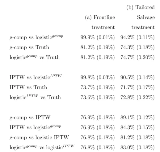
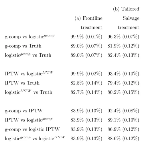
bootstrap samples), from simulated data with 5000 replicates of n=2000, stage 2 m=1600, stage 1 m=1700. . . 18 3.1 Agreement rates (se) under correct model specification. 5,000 simulations of
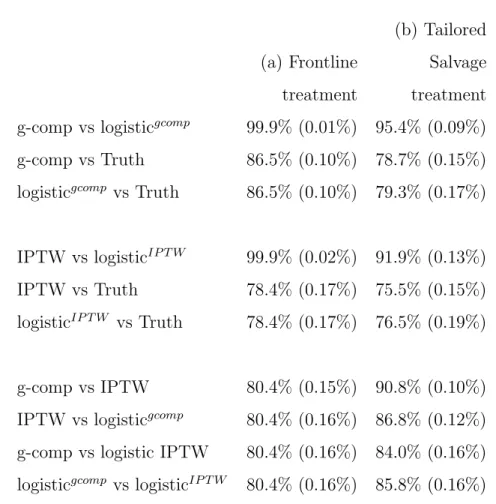
n=1,000. . . 50 3.2 Agreement rates (se) under correct model specification. 5,000 simulations of
n=2,000. . . 51 3.3 Agreement rates (se) under correct model specification. 5,000 simulations of
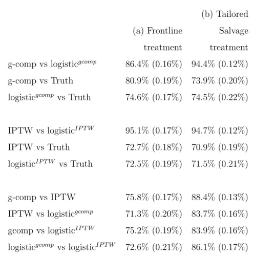
n=4,000. . . 52 3.4 Agreement rates (se) using backward selection for model building. 5,000
sim-ulations of n=1,000. . . 53 3.5 Agreement rates (se) using backward selection for model building. 5,000
sim-ulations of n=2,000. . . 54 3.6 Agreement rates (se) using backward selection for model building. 5,000
sim-ulations of n=4,000. . . 55 3.7 Initial outcomes following frontline treatment . . . 56 3.8 Outcomes following CR or Resistant Disease . . . 57 3.9 Models for sojourn time to death, time to resistance, and time to complete
3.10 Models for sojourn time from resistance to death, complete remission to disease progression, and from progression to death. . . 60
LIST OF FIGURES
2.1 True (left column) and estimated (right column) threshold utility planes for the simulated scenario. . . 20 2.2 Estimated stage 2 (top row) and stage 1 (bottom row) threshold utility planes
for COG study A3891. . . 23 3.1 Predictive vs Prescriptive Interactions . . . 29 3.2 Possible pathways, transition times, and salvage therapy following induction
treatment. . . 31 3.3 Classification model for argmax of g-computation model using the proposed
two step prescriptive variable selection method. . . 62 3.4 Forest plot of g-computation model with 90% point-wise bootstrap confidence
intervals. . . 63 3.5 Classification model for argmax of logTP D model using the proposed two step
prescriptive variable selection method. . . 65 3.6 Forest plot for logTP D model with 90% point-wise bootstrap confidence
inter-vals. . . 66 3.7 Classification model for argmax of g-computation model using the proposed
two step prescriptive variable selection method onn=1,000 simulated patients. 68 3.8 Classification model for argmax of g-computation model using the proposed
two step prescriptive variable selection method onn=1,000 simulated patients. 69 3.9 Classification model for argmax of IPTW model using the proposed two step
3.10 Classification model for argmax of IPTW model using the proposed two step prescriptive variable selection method on n=1,000 simulated patients. . . 71 3.11 Classification model for argmax of logTP D model using the proposed two step
prescriptive variable selection method on n=1,000 simulated patients. . . 72 3.12 Classification model for argmax of logTP D model using the proposed two step
PREFACE
I would like to thank my dissertation advisor, supervisor, professor, and mentor, Dr. Abdus S. Wahed. His guidance has shaped my understanding of statistical theory, and my skill in application. The opportunity to work with him and to earn my PhD has completely altered my career path, and will forever change my life. I would also like to thank Dr. Clifton D. Sutton for molding my foundation in statistical theory. My continued success rests on his training. This dissertation is dedicated to my parents, sister, wife, and son.
1.0 INTRODUCTION
Dynamic treatment regimes (DTRs) provide the basis for statistical analysis in personalized medicine. A DTR is a decision rule that guides the treatment choices over the course of therapy. The sequence of treatments a patient receives depends on the patient’s health sta-tus, response to prior treatments, and other patient characteristics [22,28,5]. The goal is to find a DTR that optimizes the overall outcome, commonly taken as overall survival in cancer studies [34, 33, 18]. Techniques for analyzing DTRs are important to properly account for patient responses and sequence of treatments to correctly identify the optimal treatment at each stage. Consider a game of chess. Each player’s turn corresponds to a stage of a DTR, each player’s move corresponds to a treatment assignment, and achieving check mate corresponds to optimizing the outcome. The player’s best move in each turn depends on his previous and future moves. If the chess player optimizes each move individually, without regard to past or future moves, he/she will likely not achieve check mate. If the treatments at each stage of a DTR are analyzed without regard to past and future treatments, biased re-sults may occur. Assuming larger outcomes are better, it is natural to search for the optimal regime, the one with the largest expected outcome. To this end there are primarily two ap-proaches: structural mean models (direct search) and nested mean models (inductive search).
Structural mean models use weighting techniques found in survey sampling to estimate the mean outcome of a regime had everyone sampled followed that regime, allowing a di-rect comparison of the outcome across DTRs. Inverse probability of treatment weighted (IPTW) estimators, as their name suggests, average the outcome for all subjects following a specific regime, while weighting each observation by the inverse of the probability of re-ceiving the treatments prescribed by the regime, similar to the Horvitz-Thompson estimator
[17]. Alternatively, g-computation estimators first find the mean outcome for each path of a particular regime, and weight these means by the proportion who followed each path to form the mean of the regime [25, 27]. Conversely, nested mean models use backwards induction to find the optimal treatment at each stage. Murhpy (2003) [22], Robins (2004) [26], and others pioneered the use of backwards induction in statistics via Q-learning and g-estimation to identify such optimal regimes. These algorithms work backwards in time by identifying at each stage which treatment has the largest expected outcome, and creating pseudo data for each subject by replacing his/her observed outcomes with the estimated optimal expected outcome at each stage, given prior observed outcomes and covariate in-formation. The optimal regime is the one with the largest expected value of this pseudo data.
Generally, to build the models that identify the optimal treatment regime clinical tri-als are designed, patients are recruited, and their information is gathered. These patients, though treated, do not get to benefit from the knowledge they collectively bring. It is the next patient in line, the prospective patient, that can use this information to make a more informed treatment decision. From the clinician’s perspective all that is required is to collect demographic, blood marker, and genetic information, and the optimal treatment regime can be assigned for the prospective patient. The prospective patient, however, has an entirely dif-ferent decision making process. He/she builds a nearly infinite dimensional model in his/her subconscious when choosing between treatments. Is the treatment painful? What are the side effects? How much does it cost? Does the treatment conflict with my ethical or religious beliefs? What is the treatment schedule and can I adhere to it? And so on. For each prospec-tive patient the questions and answers are different. From this prospecprospec-tive patient’s point of view, he/she is not here to offer a few data points, he/she is here to decide which treatment is best for him/her. To capture the decision making process of the prospective patient in the survival analysis setting, we investigate quality adjusted lifetime as the outcome in dynamic treatment regimes via Q-learning, and while this outcome is not specific to Q-learning, nor to dynamic treatment regimes, it is especially pertinent. This approach offers a glimpse into the mind of the prospective patient’s decision making process, and allows us to see just how averse the patient must be to a particular treatment, or regime, before it is no longer optimal.
Clinical trials for cancer often measure a primary outcome and several secondary out-comes. The secondary outcomes may include, among others, measures of toxicity and adher-ence. Taken separately, these measures may sometimes lead to different optimal treatments. While one treatment may have the largest expected primary outcome, a second one may be less toxic, and a third might have the best adherence. Gelber et al. (1989) [10], Glasziou et al. (1989) [11], GoldHirsch et al. (1989) [12] and Korn (1993) [19] considered quality ad-justed lifetime to adjust the length of life based on its quality. In its simplest form, quality adjusted life assigns a utility weight, ranging from 0 (death) to 1(perfect health), to separate states of health. If there are k health states, then Ui =
Pk
j=1qjsji is the quality adjusted
lifetime (QAL) for the ith patient, where s
1i, .., ski are the times spent in each state, and
q1, ..., qk are the utility coefficients assigned to each of the health states. Note that the
qual-ity adjusted lifetimeUi is simply a fraction of total lifetime for patienti. More recently, Zhao
and Tsiatis [38, 39, 40, 41] have provided consistent and efficient estimators, and provided hypothesis tests for distributional features of quality adjusted lifetime in the presence of right censoring. Wang & Zhao (2007) [35] extended this work to the regression setting, using in-verse weighting techniques to form consistent estimating equations for regression parameters.
The first goal of this dissertation is to develop an optimal dynamic treatment regime to maximize quality adjusted lifetime by using a Q-learning-type approach discussed in [18]. This method will be operationalized using the estimating equations of [35], and a threshold utility analysis will be used to show how the subject-specific optimal DTR not only depends on patient history and intermediate outcomes, but also on quality of life, monetary cost, and other factors during each treatment. Though we optimize quality adjusted lifetime, we provide suggestions on how the quality adjustment can be used for any continuous outcome via Q-learning. The utility weights capture the secondary outcomes as well as the unmeasur-able decision making process of the prospective patient and discount the expected utility of treatments. We use a simulation study to evaluate these methods, and then apply them to COG study A3891 concerning 379 children receiving treatment for high-risk neuroblastoma [21].
Dynamic treatment regimes are a function of patient data, and as ever larger studies collect more patient data, it is natural to turn to variable selection methods when search-ing for the optimal regime. Common approaches to variable selection include, but are not limited to, the forward, fackward, and ftep-wise selection methods, which by their nature are discrete processes, and the least absolute shrinkage and selection operator (LASSO) and its derivatives, which are continuous processes. To operate, all of these methods rely on a measure of model fit or prediction error, such as the sum of squared errors, the leave-one-out cross-validation estimate of prediction error, or Akaike information criterion (AIC). These variable selection methods are designed to sift through a large collection of variables and identify those that most greatly reduce the variability and increase the accuracy of the esti-mator, which Gunter et al. (2011) [13] define as predictive variables. However, in the realm of dynamic treatment regimes, we are interested in variables that are not only predictive, but also help prescribe the optimal treatment for a given patient. Such variables are called
prescriptive [15], and must qualitatively interact with treatment. For a nested mean model approach, Gunter et al. (2011) [13] propose two different ranking methods to sort variables according to how likely they will qualitatively interact with the outcome, and provide a four step algorithm involving LASSO regression on nested subsets of covariates for selecting im-portant predictive variables. Zhang (2014) [37] generalizes from the least squares regression model and offers a simpler, more effective two step method involving Multivariate Adaptive Regression Splines (MARS) models and logistic regression with LASSO.
Most authors employing structural mean models perform a marginal analysis, comparing dynamic treatment regimes for the entire sample of patients [33]. Those that perform a sub-group analysis using conditional models do so by conditioning on baseline information only [14, 5]. While these conditional models shed some light on the regime effects across baseline covariates, they lack the ability of Q-learning and other backwards induction techniques to use past and current patient information to prescribe the optimal treatment at each stage. The second goal of this dissertation is two fold: i) to propose a new method for optimiz-ing dynamic treatment regimes usoptimiz-ing conditional structural mean models that incorporates
current patient information at every stage (decision point), ii) and to provide an effective prescriptive variable selection method for these conditional structural mean models. The method in Zhang (2014) [37] for nested mean models is reviewed, and extended to structural mean models. We use a simulation study to evaluate these methods, and apply them to a phase II study concerning 215 patients with acute myeloid leukemia (AML) or high-risk myelodysplastic syndrome (MDS) [8].
2.0 QUALITY ADJUSTED Q-LEARNING AND THRESHOLD UTILITY ANALYSIS FOR OPTIMIZING DYNAMIC TREATMENT REGIMES
2.1 SETUP
2.1.1 Quality-adjusted lifetime
Describe the health history for the ith patient with a continuous time stochastic process
{Vi(t), t ≥ 0}. Vi(t) maps to the space of health states S = {0,1,2, ..., m}, where the
state ‘0’ corresponds to the absorbing state of death. Denote the health history up to time t by VH
i (t) = {Vi(s) : s ≤ t}. Let Vi(s) = 0 imply that Vi(t) = 0 for t ≥ s. Let
Ti denote the survival time for patient i. Naturally, Vi(t) = 0 for t ≥ Ti. Then we see
that Ti =inf{t :Vi(t) = 0}. Let q() be a quality of life function mapping Vi(t) to [0,1], with
q(0) ≡0. The quality adjusted lifetime for theithpatient is defined asQ(Ti) =
RTi
0 q{Vi(t)}dt.
In the presence of non-informative right censoring, one might consider the restricted survival time where total follow-up time is limited to L, where L is some value less than the maximum survival time for all patients. Therefore, the survival time for all patients will be truncated at L, TL =min(T, L). For ease of notation, we will drop the superscript and simply use T. We will denote the ith patient’s censoring time by C
i, and the survival
distribution ofC byK(t) =P(C > t). DefineUi =min(Ti, Ci) and ∆i =I(Ti ≤Ci),
respec-tively, to be the observed time to event (death or censoring), and the death indicator. Then Q(Ui) =
RUi
0 q{Vi(t)}dt represents the quality adjusted time to event for the i
In this construction the quality function q is not patient specific (does not have a sub-script i), and was assumed known. One view is that q exists at the population level. This means that every patient in the analysis, and all of the patients they represent, experience the same quality of life when in a particular health state. This allows for a threshold utility analysis, described in detail in Section 2.2.2, where quality adjusted lifetime (or a function of it) is considered over the entire range of possible values of q, to examine how the value of q affects the estimation of quality adjusted lifetime. As a convention we will take Q(s, t) to refer to Rstq{V(u)}du and Q(t) to refer to R0tq{V(u)}du.
For example, consider a discrete-state health history process Vi(t) with three states:
treatment, response (well-being), and death. Suppose each of these states are mapped to [0,1] as q{Vi(t)} = qaI{t ≤ TiR}+ 1I{TiR < t < Ti}+ 0I{t > Ti}. Such a mapping may
be reasonable as the quality is the least (zero) after death, one when healthy, and a con-stant, qa, between zero and one when being treated due to toxicity related complications
and/or monetary cost from receiving treatment A=a. Here, time from beginning of treat-ment to response is denoted by TiR. Under this scenario, Q(Ti) =
RTiR 0 qadt+ RTi TR i 1dt = Ti −(1−qa)TiR. If the patient undergoes a maintenance treatment immediately after
re-sponding, and remains on maintenance treatment B =buntil death, Q(Ti) could be written
as Q(Ti) = RTiR 0 qadt+ RTi TiRqbdt = qbTi −(qb −qa)T R
i , where the constant qb reflects the
utility weight of treatment B =b for toxicity, monetary cost, and other factors.
Since quality adjusted lifetime is the area under q{Vi(t)} over the health states from 0
to T, for any function q{Vi(t)} there exists a constant function in each health state that
results in the same area, and produces the same quality adjusted lifetime. Not coinciden-tally, the example above has the health states of each patient correspond to the sequence of treatments received. When estimating mean quality adjusted lifetime in such settings, the utility weights qa and qb factor out, producing E[Q(Ti)] = qaE[TiR] +qbE[Ti−TiR]. When
viewed in this way, not only can the utility weights be seen as population constants, they can alternatively be seen as adjustments to the expected utility of each treatment for the prospective patient, depending on his or her aversion to each treatment, with each
prospec-tive patient potentially having different values of the utility weights. Such an interpretation of the utility weights offers even more motivation for a threshold utility analysis.
For drawing inference on quality adjusted lifetime, the survival function of quality ad-justed lifetime may be used the same way as as the survival function of overall survival. In the presence of non-informative censoring one might naturally turn to the Kaplan-Meier estima-tor, to estimateS(t) =PQ(Ti)> t
, but Gelber et al. (1989) [10] and Pradhan & Dewanji (2009) [24] showed that this can result in biased estimation because the quality adjustment induces a dependence between the survival times and censoring times. Zhao & Tsiatis (1997) [38] offer an inverse-probability weighted estimator, similar to that proposed by Robins & Rotnitzky (1992) [29] and Robins et al. (1994) [30], ˆS(t)cen = 1
n Pn i=1 ∆i ˆ K(Ui)I[Q(Ui) > t], where ˆK(Ui) is the Kaplan-Meier estimator for the censoring random variable evaluated at
Ui, and ∆i and ˆK(Ui) can depend on t to improve efficiency. Zhao & Tsiatis (1999) [39]
improve the efficiency of their estimator by incorporating each patient’s health history. In Zhao & Tsiatis (2000) [40] they used the same principles to estimate the mean quality ad-justed lifetime.
Wang & Zhao (2007) [35] extended this work to the regression setting by constructing consistent estimating equations for mean quality adjusted lifetime in the presence of censor-ing, yieldingUn(β) =Pni=1 Kˆ∆(Ui
i)h(Xi){Q(Ui)−g(β, Xi)}= 0, whereXi denotes a (p+ 1)×1 vector of covariates associated with patient i, with the first covariate being the constant 1, h(Xi) is a (p+ 1)×1 vector of functions of Xi,β is a (p+ 1)×1 vector of parameters, and
g(β, Xi) = E[Q(Ti)|Xi]. The estimator for β solving Un(β) will be used to operationalize
our search for the optimal dynamic treatment regime, described in Section 2.2.
2.1.2 Dynamic treatment regimes and corresponding terminology
Consider a two-stage sequential multiple assignment randomized trial (SMART) design where patients are randomized to one of two induction therapies, A = {a1, a2}. Patients may be
if treatment response is observed, patients are further randomized to one of two maintenance treatments, B={b1, b2}. This design allows for inference on four DTRs that might be
car-ried out in clinical practice, namely, d(Ai =aj;Bi =bk), j, k = 1,2, where d(Ai;Bi) stands
for “Treat with Ai, if the patient responds, treat with Bi.” Our goal is to find the optimal
treatment regime among these that maximizes expected quality adjusted lifetime.
Let GHi (t) denote all information collected on patient i prior to time t. Some or all of the information in GH
i (t), for example serum biomarker levels, responses to questionnaires,
or tumor size, is used to defineViH(t), which then defines Ri andTiR, the observed response
indicator and the observed time to response given Ri = 1, respectively. GHi (t) may include
additional patient information not used to defineViH(t). Then, introducing further indicators for first and second stage treatment, the observed data for the ith patient in the presence of
censoring is written as Diδ =Z1(Ai), Z2(iA), Ri, RiTiR, RiZ (B) 1i , RiZ (B) 2i , Ui, ∆i, ViH(Ui), GHi (Ui) ,
where Zji(A)=1 if patient i received the jth induction therapy, Zji(A)=0 otherwise, and Zki(B) denotes the bk treatment assignment indicator I{B = bk}, defined only if Ri=1. Note that
Z2(Ai ) = 1−Z1(Ai) and Z2(Bi ) = 1−Z1(Bi ), but we explicitly define them to facilitate the use of summation.
By design, treatments are assigned independently of prognosis or any observed data measured prior to the second stage. This condition is often referred to as no unmeasured confounders or sequential randomization assumption. This ‘no unmeasured confounders’ condition holds even if the second-stage randomization probabilities depend on the first-stage treatment assignments.
2.2 OPTIMIZATION OF DYNAMIC TREATMENT REGIMES ON QUALITY ADJUSTED SURVIVAL
2.2.1 Optimization
Following the work of Murphy (2003) [22], Robins (2004) [26], and Huang et al. (2014) [18], we describe a backward induction method to identify the optimal dynamic treatment regime, using mean quality adjusted survival time as the criterion of optimality. From the reinforcement learning literature in the field of DTRs, the typical Q-functions for two stages of our SMART design, assuming no unmeasured confounders, would be
QB Ai =aj, GHi (T R i ), Bi =bk = EhQ(TiR, Ti) Ai =aj, Ri = 1, G H i (T R i ), Bi =bk i QA GHi (0), Ai =aj = EhHi(A) G H i (0), Ai =aj i , where Hi(A) = Q(TR i ) +maxb k QB Ai, GHi (TiR), Bi =bk , if Ri = 1 Q(Ti), if Ri = 0.
Then, the optimal stage 1 treatment given baseline information is
Aopti =argmax ak EhHi(A) G H i (0), Ai =aj i ,
and the optimal stage 2 treatment given stage 1 treatment assignment and information up to stage 2 is Biopt =argmax bk EhQ(TiR, Ti) Ai =aj, Ri = 1, G H i (T R i ), Bi =bk i .
Below we walk through the backwards induction used to estimate the optimal treatment at each stage, with a differentHi(A) shown in Huang et al. (2014) that we use in our simulation and application.
We start with the second stage (include only those patients who responded Ri = 1).
therapy to death for those patients who responded is Q(TR i , Ti) = RTi TR i q{Vi(t)}dt, so that γB ≡ E Q(TiR, Ti) Ai =aj, Bi =b1, Ri = 1, GHi (T R i ) −E Q(TiR, Ti) Ai =aj, Bi =b2, Ri = 1, GHi (T R i )
is the difference in expected stage 2 outcomes, given prior information. We assume the following linear model for QB
Ai, Bi, Ri = 1,X¯Bi,βB,αB E Q(TiR, Ti) Ai, Bi, Ri = 1,X¯Bi,βB,αB = ¯XBi0 βB+Z1(iB)X¯Bi0 αB, (2.1)
where ¯XBi are the first stage treatment assignment indicators and covariates fromGHi (TiR),
and includes an element equal to 1 corresponding to an intercept term, which implies that γB = ¯XBi0 αB, and the estimated optimal stage two treatment given stage 1 treatment
as-signment and patient information up to stage 2 is ˆ Bopt( ¯XBi) =argmax bk ˆ E Q(TiR, Ti) Ai =aj, Ri = 1, Bi =bk,X¯Bi,βB,αB .
If γB is positive then b1 is the optimal stage 2 treatment, otherwise, b2 is optimal. Using
fitted models corresponding to equation (2.1) we can estimate the optimal quality adjusted time from maintenance therapy to death as
Hi(B)( ˆαB)≡ Q(TiR, Ti) + ¯ XBi0 αˆB , if Bi =bk, ˆ Biopt 6=bk Q(TR i , Ti), if Bi =bk, Bˆiopt =bk.
Moving to the first stage, under assumptions described in Section 2.1.2 the quality ad-justed survival time with observed stage one treatment and the estimated optimal stage two treatment can be written as
Hi(A)( ˆαB) = Q(TR i ) +H (B) i ( ˆαB), if Ri = 1 Q(Ti), if Ri = 0.
the following linear model for QA Ai, XAi,βA,αA E h Hi(A)( ˆαB) Ai, XAi,βA,αA i =XAi0 βA+Z1(iA)XAi0 αA,
whereXAi includes an element equal to 1 corresponding to an intercept term, which implies
that γA ≡EhHi(A)( ˆαB) Ai =a1, G H i (0) i −EhHi(A)( ˆαB) Ai =a2, G H i (0) i =XAi0 αA
is the difference in expected outcomes at stage 1, given that each patient received his esti-mated optimal stage 2 treatment. The estiesti-mated optimal stage one treatment is
ˆ Aopt(XAi) = argmax aj ˆ E Hi(A)( ˆαB) Ai =aj, XAi,βA,αA .
If γA is positive thena1 is the optimal stage 1 treatment, otherwise, a2 is optimal. Thus if
one could estimate the quantities γA orγB, or equivalently, the parameters αB and αA, the
optimal treatment regime could be constructed given the q function for each specific stage.
To estimate these parameters, the simple weighted regression models described in Section 2.1.1by Wang & Zhao (2007) [35] can be used. Explicitly, for stage 2 we solve the estimating equation U(B) n (βB,αB) = n X i=1 ∆i ˆ K(Ui) Ri ¯ XBi Z1(Bi )X¯Bi n Q(TiR, Ui)−X¯ 0 BiβB−Z (B) 1i X¯ 0 BiαB o = 0,
for βB and αB. Similarly, for stage 1 we solve
U(A) n (βA,αA) = n X i=1 ∆i ˆ K(Ui) XAi Z1(Ai)XAi n Hi(A)(αˆB)−X 0 AiβA−Z (A) 1i X 0 AiαA o = 0
to obtain estimates of βA and αA.
2.2.2 Threshold Utility Analysis
Glasziou et al. (1990) [11] perform a threshold utility analysis when studying the effects of adjuvant chemotherapy on quality adjusted lifetime in patients with early breast cancer.
Each patient’s survival time is quality adjusted based on periods of toxicity of treatment and relapse of disease. These quality weights, ranging from 0 to 1, are plotted against each other and the regions where each treatment is favored are identified via lines (planes) of indifference. This results in a type of sensitivity analysis, allowing one to see all possible treatment decisions drawn depending on the quality weights. In our DTR setting, a patient’s course of treatment often depends on his/her state of health, be it response to treatment or relapse of the disease, so that his/her health states correspond to the stages of the DTR. In our approach, each patient’s survival time will be weighted according to treatment received, allowing a threshold utility analysis among treatments, and ultimately among regimes.
Optimal decision rules for first and second stage treatments developed in Section 2.2 are not only a function of the observed data (patient level information), but also of the quality of life functionq. In our development in the previous section, we assumed that this q function was known, and we offered two interpretations of its meaning. Rather than performing a single analysis with one q function, a sensitivity analysis can be performed using a variety of reasonable q functions to determine for which functions ofq, if any, the choice of optimal regime changes. In the special case of constant q functions, q can be varied from 0 to 1, and a threshold utility plane can be plotted. This is of importance, since depending on the values of the q function, there may be different optimal treatment regimes.
To be explicit, consider quality adjusting each patient’s survival time as
Q(Ti) = Tiqaj ,if Ai =aj, Ri = 0, TR i qaj + (Ti−T R i )qbk ,if Ai =aj, Ri = 1, Bi =bk,
for j = 1,2, k = 1,2 where qaj, qbk ∈[0,1]. For those who responded (Ri = 1) and received maintenance treatment, the quality weightsqb1, qb2 ∈[0,1] can be plotted against each other
on the xand y axes, with ˆ γB = Eˆ (Ti−TiR)qb1 Ai =aj, Bi =b1, Ri = 1,X¯Bi,βB,αB −Eˆ (Ti−TiR)qb2 Ai =aj, Bi =b2, Ri = 1,X¯Bi,βB,αB = X¯Bi0 αˆB
from Section 2.2 plotted on the z axis. This forms a two-dimensional plane in a three-dimensional space. When quality adjusting in this way, the utility weights qb1 and qb2 factor out of the expectations and can be viewed as adjustments to the expected utility of each stage two treatment for the prospective patient, depending on his or her aversion to each treatment. The line where ˆγB = 0 is the estimated threshold at which the expected utility of b1 and b2 are equal, where the prospective patient is indifferent when choosing between
stage two treatments.
Similarly, for those who received an induction treatment, the quality weights qa1, qa2 ∈ [0,1] can be plotted against each other on thex and y axes, with
ˆ γA= ˆEhHi(A)(αˆB) Ai =a1, XAi,βA,αA i −EˆhHi(A)(αˆB) Ai =a2, XAi,βA,αA i =XAi0 αˆA
from Section 2.2 plotted on the z axis, where
Hi(A)(αˆB) = TR i qaj +H (B) i (αˆB), if Ai =aj, Ri = 1 Tiqaj, if Ai =aj, Ri = 0 Hi(B)(αˆB) = (Ti−TiR)qbk + ¯ XBi0 αˆB , if Bi =bk, ˆ Biopt6=bk (Ti−TiR)qbk, if Bi =bk, Bˆ opt i =bk.
The line where ˆγA = 0 is the estimated threshold at which the prospective patient is indif-ferent when choosing between a1 and a2.
2.2.3 Inference
Robins (2004) [26], Chakraborty et al. (2009) [6], and Laber et al. (2014) [20] are quick to point out that the estimators derived from Q-learning have non-regular limiting distribu-tions, because the estimated stage 1 pseudo data (and hence the estimated stage 1 model parameters) are a non-smooth (non-differentiable at ¯XBi0 αˆB=0) function of αˆB. This
mo-tivated Chakraborty et al. (2013) [4] to discuss the m-out-of-n bootstrap in the context of DTRs, in place of standard large-sample inference methods. The m-out-of-n bootstrap technique essentially smooths the empirical distribution function, with more smoothing cor-responding to smaller values of m, the resample size, by allowing the empirical distribution function to tend to its limiting distribution at a faster rate than the bootstrap empirical distribution tends to the empirical distribution. We use this technique to create confidence regions in the threshold utility analysis, identifying regions of indifference and strong ac-ceptance when choosing between stage 1 and stage 2 treatments. While Chakraborty et al. (2013) [4] provide several data driven methods for determining the smaller resample size m, we find a suitablem through simulation and apply this same m in the analysis of real data.
2.3 SIMULATION STUDY
In this section we conduct a simulation experiment to evaluate the optimization of dynamic treatment regimes for quality adjusted lifetime described in Section2.2. Similar to the COG study A3891 that will be presented later in Section2.4, we consider a 2-stage SMART design.
We generated 5,000 simulations with sample size n=1000. Patients are randomized to one of two induction therapies with probability one-half, and the probability of non-response for each induction therapy is the same, 0.55. Those who respond to induction therapy are further re-randomized with probability one-half to one of two maintenance therapies. So-journ times to response and/or death were generated from various exponential distributions.
Table 2.1 shows the coverage probabilities over the 5,000 simulations for 90% point-wise bootstrap confidence intervals for the estimated difference in mean quality adjusted lifetime between Stage 1 and Stage 2 treatments (γA and γB, respectively) when searching for the
optimal treatment regime using the simple weighted estimating equations from Section2.1.1. The 5thand 95thpercentiles of the bootstrapped sampling distributions are used to create the
confidence intervals. Stage 1 coverage probabilities are estimated at qb1 = 0.8 and qb2 = 0.6. A variety of re-sample sizes were considered for the stage 1m-out-of-nbootstrap, and m=850 produced confidence intervals maintaining the nominal coverage probability. The coverage probabilities for the 90% confidence intervals are close to the nominal level for utility weights that are away from zero. This makes sense, as a value of q close to zero greatly reduces the variability in the data, making it difficult to estimate the respective quantities. For some combinations of qb1 and qb2 the estimated stage 2 coverage probabilities are below the nom-inal level. Although no irregularity issues exist for the stage 2 estimates, the m-out-of-n bootstrap was still employed to improve the coverage probabilities, with m=800. Using the m-out-of-n bootstrap, the stage 1 coverage probabilities for the difference in mean quality adjusted lifetime are well maintained. Similar simulations were performed with a sample size ofn=300 and survival times close to that of the COG study A3891. This gives us an idea of an appropriate choice of m. We found thatm=240 and m=255 worked well for maintaining the nominal coverage probabilities for stage 2 and stage 1, respectively.
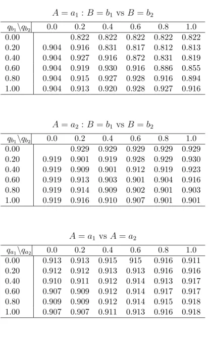
Table 2.1: Coverage probabilities of 90% point-wise bootstrap confidence intervals (500 bootstrap samples), from simulated data with 5000 replicates of n=1000, stage 2 m=800, stage 1 m=850. A=a1 : B =b1 vs B =b2 qb1\qb2 0.0 0.2 0.4 0.6 0.8 1.0 0.00 0.822 0.822 0.822 0.822 0.822 0.20 0.904 0.916 0.831 0.817 0.812 0.813 0.40 0.904 0.927 0.916 0.872 0.831 0.819 0.60 0.904 0.919 0.930 0.916 0.886 0.855 0.80 0.904 0.915 0.927 0.928 0.916 0.894 1.00 0.904 0.913 0.920 0.928 0.927 0.916 A=a2 : B =b1 vs B =b2 qb1\qb2 0.0 0.2 0.4 0.6 0.8 1.0 0.00 0.929 0.929 0.929 0.929 0.929 0.20 0.919 0.901 0.919 0.928 0.929 0.930 0.40 0.919 0.909 0.901 0.912 0.919 0.923 0.60 0.919 0.913 0.903 0.901 0.904 0.916 0.80 0.919 0.914 0.909 0.902 0.901 0.903 1.00 0.919 0.916 0.910 0.907 0.901 0.901 A=a1 vs A=a2 qa1\qa2 0.0 0.2 0.4 0.6 0.8 1.0 0.00 0.913 0.913 0.915 915 0.916 0.911 0.20 0.912 0.912 0.913 0.913 0.916 0.916 0.40 0.910 0.911 0.912 0.914 0.913 0.917 0.60 0.907 0.909 0.912 0.914 0.917 0.917 0.80 0.909 0.909 0.912 0.914 0.915 0.918 1.00 0.907 0.907 0.911 0.913 0.916 0.918
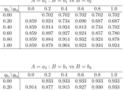
Table 2.2: Coverage probabilities of 90% point-wise bootstrap confidence intervals (500 bootstrap samples), from simulated data with 5000 replicates of n=2000, stage 2 m=1600, stage 1 m=1700. A=a1 : B =b1 vs B =b2 qb1\qb2 0.0 0.2 0.4 0.6 0.8 1.0 0.00 0.702 0.702 0.702 0.702 0.702 0.20 0.859 0.924 0.734 0.690 0.687 0.687 0.40 0.859 0.914 0.924 0.813 0.734 0.702 0.60 0.859 0.897 0.927 0.924 0.857 0.780 0.80 0.859 0.884 0.914 0.932 0.924 0.878 1.00 0.859 0.878 0.904 0.923 0.934 0.924 A=a2 : B =b1 vs B =b2 qb1\qb2 0.0 0.2 0.4 0.6 0.8 1.0 0.00 0.933 0.933 0.933 0.933 0.933 0.20 0.914 0.877 0.915 0.927 0.930 0.933 0.40 0.914 0.896 0.877 0.901 0.915 0.923 0.60 0.914 0.901 0.890 0.877 0.891 0.910 0.80 0.914 0.907 0.896 0.885 0.877 0.886 1.00 0.914 0.907 0.889 0.892 0.884 0.877 A=a1 vs A=a2 qa1\qa2 0.0 0.2 0.4 0.6 0.8 1.0 0.00 0.915 0.918 0.918 0.915 0.912 0.908 0.20 0.910 0.913 0.916 0.917 0.915 0.911 0.40 0.905 0.910 0.911 0.914 0.914 0.915 0.60 0.905 0.908 0.911 0.911 0.916 0.914 0.80 0.903 0.904 0.908 0.912 0.913 0.915 1.00 0.900 0.901 0.905 0.910 0.912 0.914
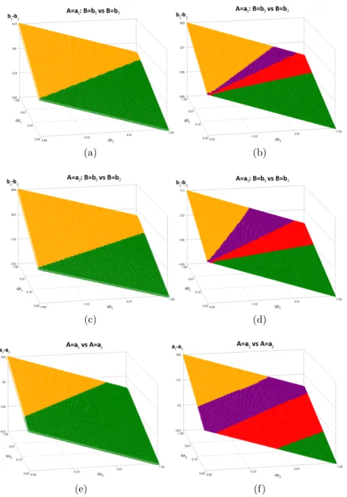
Figure 2.1 shows the true (left column) and estimated (right column) threshold utility planes for the simulated scenario with n=300. The estimated threshold utility planes are for a single simulated data set. For each combination of qb1 and qb2, or qa1 and qa2, the estimated difference in mean quality adjusted lifetime is plotted. The yellow and green represent the region of strong acceptance for choosing between b1 and b2, or a1 and a2,
respectively. The purple and red near the center of the plane have 90% point-wise bootstrap confidence intervals that cover zero and represent the region of indifference when choosing between b1 and b2, or a1 and a2. We see that for the estimated threshold utility planes, the
estimated line of indifference does not correspond exactly with the true line of indifference, yet the 90% confidence region does contain the true line. These threshold utility planes allow us to visualize how the optimal regime changes depending on the values ofqb1,qb2,qa1, and qa2. For example, assume that the threshold utility planes presented on the right panel of Figure2.1 are the planes computed from the observed data. If for these treatmentsqa1=0.8, qa2=0.5, qb1=0.7, and qb2=0.5, then the estimated optimal regime is d(A = a1;B = b1). However, if qa1=0.3, qa2=0.8, qb1=0.4, and qb2=0.6, the estimated optimal regime would be d(A=a2;B =b2).
(a) (b)
(c) (d)
(e) (f)
Figure 2.1: True (left column) and estimated (right column) threshold utility planes for the simulated scenario.
2.4 APPLICATION WITH THRESHOLD UTILITY ANALYSIS
In this section we apply the optimization methods discussed previously to the COG study A3891 concerning 379 children ages 6-months to 17 years old receiving treatment for high-risk neuroblastoma. All 379 patients were to receive five cycles of chemotherapy before begin-ning their induction treatment. Of these, 189 patients were randomized to receive continued chemotherapy (three additional cycles), A = a1, and the remaining 190 were randomized
to receive bone marrow transplantation, A = a2. After completing the induction therapy,
203 patients were deemed responders (those for whom the disease did not progress) and consented to further randomization to receive six cycles of 13-cis-retinoic acid (160 mg per square meter per day for 14 consecutive days), B =b1, or no further therapy, B =b2.
Sur-vival time was truncated to 2452 days, since this was the largest observed death time in the study.
In what follows we assume the role of the prospective patient, considering only quality of life as affected by toxicity of treatment when choosing between treatments. Each of the therapies in this study comes with its own side effects. Following a cohort of lung cancer pa-tients undergoing chemotherapy, Winter et al. (2013) [36] measured quality of life using the EORTC QLQ-C30 questionaire [1] as the patients completed multiple courses of chemother-apy. In the analysis by Winter et al. (2013) [36], the highest average global quality of life measure (ranging 0 to 100) over multiple courses of chemotherapy was 57. We rescaled these scores between 0 and 1 to have the quality of life weight of those undergoing chemother-apy vary between 0.5 to 0.6. In the case of bone marrow transplant, Felder et al. (2006) [9] analyze the health related quality of life of 68 pediatric patients aged 4 to 18 years old receiv-ing allogeneic bone marrow or stem cell transplantation in a 5-year prospective study usreceiv-ing The Pediatric Quality of Life Inventory(PedsQL) and The Health Utilities Index Mark2 + 3(HUI2/3). It is reasonable to interpret these scores as quality weights, indicating that those undergoing bone marrow transplantation have a quality of life near 0.7. Hong et al. (1986) [16] studied the use of 13-cis-retinoic acid in 44 patients with oral leukoplakia, and found
that cheilitis, erythema, and dry skin were most common. Based on the symptoms, mean survival time for patients on 13-cis-retinoic acid could reasonably be quality adjusted by 0.9.
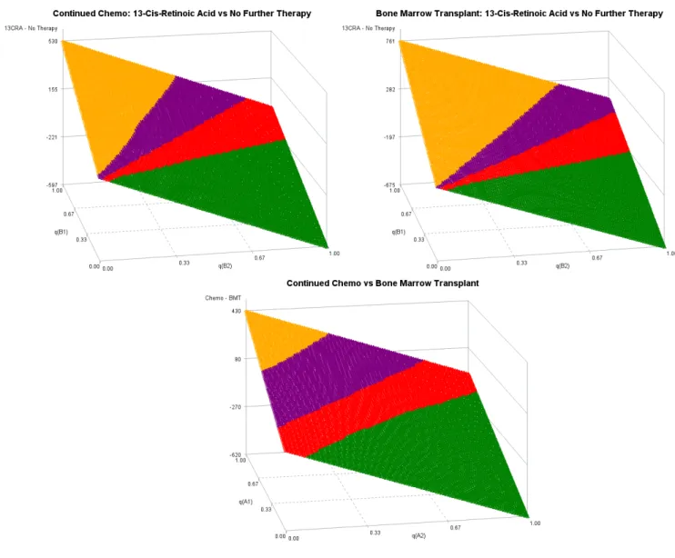
Figure2.2 (top row) shows the estimated stage 2 threshold utility planes - the estimated mean survival time for those on 13-cis-retinoic acid minus the estimated mean survival time for those on no further treatment. The yellow and green represent the region of strong ac-ceptance for 13-cis-retinoic acid and no further therapy, respectively. The purple and red near the center of the plane give point estimates that favor 13-cis-retinoic acid and no fur-ther fur-therapy, respectively, but the 90% point-wise bootstrap confidence intervals cover zero and represent the region of indifference when choosing between 13-cis-retinoic acid and no further therapy.
When the survival times for stage 2 treatments are both given a weight of 1 (no quality adjustment), those who received no further therapy had larger survival times than those who received 13-cis-retinoic acid, following continued chemotherapy; following bone marrow transplant, those who received 13-cis-retinoic acid had, on average, larger survival times than those who received no further therapy. It should be noted, though, that both of these point estimates fall within the m-out-of-n bootstrap indifference regions (the red and purple shaded areas), suggesting there is no statistically significant difference between the stage 2 treatments following either stage 1 treatment.
As one would begin to lower either qb1 orqb2 towards 0, while holding the other fixed, we see that the estimated difference in mean quality adjusted survival time falls in the region of statistical significance, where one stage 2 treatment truly out performs the other, given the stage 1 treatment. For qb1=0.9 and qb2=1, the stage 2 quality of life weights considered earlier for this study, the point estimate for the optimal stage 2 treatment falls in the same region as that for qb1=1 and qb2=1 described above and yields 13-cis-retinoic acid for those following bone marrow transplantation, and no further therapy for those following continued chemotherapy. If qb1 is lower than 0.9, the optimal stage 2 treatment would be no further therapy for both induction therapies.
Figure 2.2: Estimated stage 2 (top row) and stage 1 (bottom row) threshold utility planes for COG study A3891.
Figure 2.2 (bottom row) also shows the estimated stage 1 threshold utility plane - the estimated mean survival time for those on continuation chemotherapy minus the estimated mean survival time for those who received a bone marrow transplant. This figure is generated using pseudo data where responders at stage 1 are assumed to take their optimal stage 2 treatment, and their remaining survival time is estimated using the methods from Section
2.2, with qb1=0.9 for 13-cis-retinoic acid and qb2=1 for no further treatment. Atqa1=0.5 and qa2=0.7 the optimal stage 1 treatment is bone marrow transplant, and the point estimate falls within the strong acceptance region, meaning the 90% point-wise bootstrap confidence interval for the difference in mean survival time between continued chemotherapy and bone marrow transplant does not contain zero. Therefore, with qa1=0.5, qa2=0.7, qb1=0.9, and qb2=1, the optimal regime is to first treat with bone marrow transplantation and, if a response is observed, treat with 13-cis-retinoic acid.
2.5 GENERALIZATION TO OTHER OUTCOMES
Our exploration of Q-learning to optimize a dynamic treatment regime on quality adjusted lifetime leads one to consider Q-functions that weight the expected utility at each stage for any continuous outcome, not just survival time. For a 2-stage SMART design depicted earlier with a primary outcomeY at the end of the second stage, one can use theQ-functions
QB Ai =aj,X¯Bi, Bi =bk =qbkE h Yi(B) Ai =aj, ¯ XBi, Bi =bk i , (2.2) QA XAi, Ai =aj =EhHi(A) XAi, Ai =aj i , (2.3) where Hi(A) = Yi(A)qaj +max bk QB Ai =aj,X¯Bi, Bi =bk, , if Ai =aj, Ri = 1 Yi(A)qaj, if Ai =aj, Ri = 0, (2.4)
and whereYi(A) and Yi(B) are the outcomes at the first and second stages, respectively, with Yi(A) +Yi(B) = Yi. The law of total expectation can be used to improve computational
efficiency when performing a threshold utility analysis. Most authors fit a single regression model for EhHi(A)
XAi, Ai = aj i
using EhHi(A) XAi, Ai =aj i =P(Ri = 1|XAi, Ai =aj) ×nqajE h Yi(A) XAi, Ai =aj i +Ehmax bk QB Ai =aj,X¯Bi, Bi =bk XAi, Ai =aj io +P(Ri = 0|XAi, Ai =aj) n qajE h Yi(A) XAi, Ai =aj, io . (2.5)
Written this way, it is clear how the utility weights factor out of the expectations and create what we call quality adjusted Q-learning, for any continuous outcome. This could easily be generalized to SMARTs with an arbitrary number of stages. ModelingEhHi(A)
XAi, Ai =aj i
in this way improves computational efficiency since each of the component models only needs to be fit once before varying the utility weights and producing a threshold utility analysis. Other authors, including Song et al. (2011) [31], consider Q-functions that have a single utility weight q, regardless of stage or treatment, that is multiplied to every nested expec-tation (except the first), creating an effect similar to the autoregressive working correlation structure from generalized linear models. Most authors interpret this single q as a utility weight that, when compounded over the nested expectations, diminishes the expected utility of each subsequent stage. The idea being that the prospective patient might not complete every stage of the DTR, and the optimal regime should give more importance to earlier treat-ments. However, even with this approach, most authors ignore the utility weight by setting it equal to 1. As we showed above, we propose assigning a separate utility weight to each treatment of each stage, representing the prospective patient’s aversion to each treatment based on discomfort, side effects, monetary cost, ethical and/or religious beliefs, ability to complete the treatment schedule, and a host of other unmeasurable factors that might vary from one prospective patient to another. This allows a threshold utility analysis as described in Section2.2.2 for any continuous outcomeY, and shows us the decision making process of the prospective patient.
2.6 CONCLUDING REMARKS
Quality adjusted lifetime is a natural endpoint for deciding among treatments that prolong survival time, permitting the prospective patient to factor toxicity and financial burden of treatment, among other factors, into the decision. This is particularly useful in the realm of DTRs, allowing the optimal regime to depend not only on patient level characteristics, but also on treatment characteristics. We have demonstrated how threshold utility analysis can be combined with the standard optimization algorithm to produce optimal regimes account-ing for patient and treatment level information. For simplicity, our methods did not include any covariate information other than response status, but additional patient characteristics such as age, race, or sex could be included in the optimization algorithm, producing a sep-arate set of utility planes for, say, males and females, or young children and older children. Patient information could also be used to improve efficiency by using the semiparametric estimating equations in Wang & Zhao (2007) [35].
3.0 CONDITIONAL STRUCTURAL MEAN MODELS AND VARIABLE SELECTION FOR OPTIMIZING DYNAMIC TREATMENT REGIMES
3.1 LINEAR REGRESSION AND VARIABLE SELECTION
3.1.1 Background
For observationsY = [Y1, Y2, ..., Yn]T, a least squares linear regression model takes the form
Y =Xβ+, (3.1)
where is a n-dimensional mean zero random vector of errors, β is a (p+ 1)-dimensional vector of parameters, and X is an n×(p+ 1) design matrix of covariates, with a vector of 1’s corresponding to an intercept. The parameter estimates are obtained by minimizing the sum of squared errors
SSE =
n
X
i=1
(Yi−Yˆi)2, (3.2)
where ˆYi = xTi β. If the total number of covariates is large, one would naturally want toˆ
select the best subset of variables that explain the mean outcome. Not only isSSE used to find the line of best fit for a given model, it is also useful for goodness-of-fit when examining competing models and possible interaction effects. The model with smaller sum of squared errors fits the data best.
Other goodness-of-fit information criteria, such as AIC,BIC, and Mallow’sCp statistic,
use SSE for model comparison while incorporating a penalty for increasing the number of model parameters. Allen (1974) [2] introduced the leave-one-out cross-validation estimate
of prediction error, CV, in the context of linear regression. Many other cross-validation cri-teria have been proposed since. The model with the smallest value of such a cricri-teria should provide a good fit for another independent sample of data, that is, the model will have good out-of-sample prediction. It should also be noted that the p-values resulting from F or χ2
tests of model parameters may also be used when choosing between competing models.
When using any of the above criteria for model selection, it may be infeasible to sys-tematically search for the best subset of variables and interactions, simply because of the sheer number of variables available. In these cases there are several traditional and penalized variable selection methods that are computationally more efficient, though not guaranteed to produce the best subset. Such discrete methods include forward, backward, and stepwise variable selection. Other continuous variable selection methods include the least absolute shrinkage and selection operator (LASSO) and its derivatives. The model comparison cri-teria and variable selection methods above are not limited to least squares linear models. They work equally well for other regression models such as generalized linear models and regression splines.
3.1.2 Quantitative vs Qualitative Interactions and Variable Selection
These variable selection methods help to find the covariates and their interactions that are predictive when estimating the expected value of Yi, but do not clearly identify for which
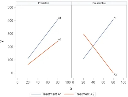
values of the covariates the choice of optimal treatment changes, where we take the optimal treatment to be the one with the largest expected outcome. Gunter et al. (2011) [13] define predictive variables as those used to reduce the variability and increase the accuracy of the estimator, whereas variables that help prescribe the optimal treatment for a given patient are called prescriptive [15]. When estimating the mean outcome, it is best to collect as many predictive variables as possible; however, only those predictive variables that are also prescriptive are needed when deciding between treatments (Figure 3.1). In order for a variable to be prescriptive, it must qualitatively interact with treatment. A variable X is said to qualitatively interact with the treatment Z if there exists at least two distinct
non-empty sets within the space ofX for which the optimal treatment is different. That is, there exists disjoint, non-empty sets S1, S2 ⊂space(X) for which
argmax Z
E[Y|X =x1, Z =z]6=argmax
Z
E[Y|X =x2, Z =z],
for all x1 ∈S1 and x2 ∈S2.
Figure 3.1: Predictive vs Prescriptive Interactions
Working in the single-stage setting using backwards induction, Gunter et al. (2011) [13] propose two different ranking methods to sort variables according to how likely they will qualitatively interact with treatment, and provide a four step algorithm involving LASSO regression on nested subsets of covariates for selecting important predictive variables. Fol-lowing their work, Zhang (2014) [37] generalizes from the least squares regression model and considers models of the form
E[Yi|Xi, Zi] =h(Xi,β) +Zi ×u(Xi,α), (3.3)
whereZi ∈ {1,−1}is a treatment assignment indicator, andu(Xi,α) are interaction effects
adaptive regression spline (MARS) models are used to fit a nonparametric model on the outcome of interest and simultaneously select predictive (and prescriptive) variables from a larger subset of variables, and (ii) the sign of the interaction contrasts is used to create a bi-nary variable indicating the optimal regime for each subject, and penalized logistic regression with LASSO (L1-logistic regression) is used to identify which of the significant interactions
are not only predictive, but also prescriptive. The use of a MARS model in the first step is warranted if we do not care about interpretability of model parameters, but are primarily interested in the predicted outcome given the covariates.
As will be seen in Section3.4 in the context of survival analysis in a two stage sequential multiple assignment randomized trial (SMART) design, a similar two step method can be used to identify important qualitative interactions for structural mean models. We consider a specific two stage setting, similar to that used in our application, but the methods described easily extend to other DTR setups.
3.2 DYNAMIC TREATMENT REGIMES AND CORRESPONDING
TERMINOLOGY
Consider a two-stage sequential multiple assignment randomized trial (SMART) design where patients are randomized to one of four induction therapies, A ={a1, a2, a3, a4}. A patient
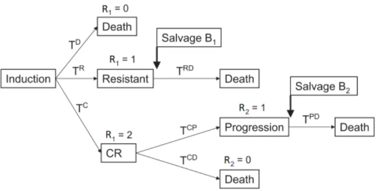
could die, the disease could become resistant to the initial treatment, the patient could re-spond (complete remission), or he/she could experience disease progression after complete remission. For each of the induction therapies, if treatment resistance or progression following complete remission is observed, patients are further randomized to one of two salvage treat-ments, B={b1, b2}. This design allows for inference on sixteen DTRs that might be carried
out in clinical practice, namely, d(Ai =aj;B1i =bk, B2i =bl), j = 1, ...,4, k= 1,2, l= 1,2
where d(Ai;B1i, B2i) stands for “Treat with Ai; if the patient is resistant to Ai, treat with
progres-sion, treat with B2i.” Our goal is to find the optimal treatment regime among these that
maximizes expected survival time.
Figure 3.2: Possible pathways, transition times, and salvage therapy following induction treatment.
Let TD
i , TiR, TiRD, TiC, TiCP, and TiP D, TiCD, respectively denote the observed time to
death if neither remission nor resistance was observed, the observed time to resistance and the observed time from resistance to death if resistance is observed, the observed time to complete remission, the observed time from complete remission to disease progression, the observed time from progression to death, and the observed time from complete remission to death if complete remission is observed. Using the above sojourn times, each patient’s survival time can be expressed as
Ti = TD i , R1i = 0 TR i +TiRD, R1i = 1 TC i +TiCP +TiP D, R1i = 2, R2i = 1 TC i +TiCD R1i = 2, R2i = 0,
where R1i indicates whether a patient fails, is resistant, or experiences complete remission,
andR2i indicates whether or not those that experienced complete remission later experience
In the presence of non-informative right censoring, one might consider the restricted survival time where total follow-up time is limited toL, where Lis some value less than the maximum survival time for all patients. Therefore, the survival time for all patients will be truncated atL,TL=min(T, L). For ease of notation, we will drop the superscript and simply
use T. We will denote the ith patient’s censoring time by C
i, and the survival distribution
of Ci byK(t) = P(Ci > t). Define Ui =min(Ti, Ci) and ∆i =I(Ti ≤Ci), respectively, to be
the observed time to event (death or censoring), and the death indicator. It is possible that Ci < Ti, so that for a single patient some of the sojourn times are censored while others are
observed. Therefore,Ui can be expressed as
Ui = UD i , R1i = 0 TiR+UiRD, R1i = 1 TC i +TiCP +UiP D, R1i = 2, R2i = 1 TiC +UiCD R1i = 2, R2i = 0,
where R1i=0 if a patient fails or is censored prior to observing R1i; R2i=0 if a patient dies
after complete remission or is censored after complete remission prior to observing R2i; UiD
= min(TD
i , Ci) and ∆Di = I(TiD ≤ Ci); UiRD = min(TiRD, Ci −TiR) and ∆RDi = I(TiRD ≤
Ci−TiR); UiP D = min(TiP D, Ci−TiCP −TiC) and ∆P Di = I(TiP D ≤ Ci−TiCP −TiC); UiCD
= min(TCD
i , Ci−TiC) and ∆CDi =I(TiCD ≤Ci−TiC). Then, introducing further indicators
for first and second stage treatment, the observed data for the ith patient in the presence of censoring is written as Dδi =Zji(A), R1i, I{R1i = 2}R2i, I{R1i = 0}UiD, I{R1i = 1}TiR, I{R1i = 1}Z (B1) ki , I{R1i = 1}UiRD, I{R1i = 2}TiC, I{R1i = 2}I{R2i = 1}TiCP, I{R1i = 2}I{R2i = 1}Z (B2) li , I{R1i = 2}I{R2i = 1}UiP D, I{R1i = 2}I{R2i = 0}UiCD, Ui, ∆i, ∆Di , ∆ RD i , ∆ P D i , ∆ CD i , G H i (Ui) , j = 1,2,3,4, k, l= 1,2,
where Zji(A)=I{Ai =aj} equals 1 if patient i received thejth induction therapy, Z
(A)
0 otherwise, Z(B1)
ki =I{B1i = bk} and Z
(B2)
li =I{B2i = bl} denote the salvage treatment
as-signment indicators, defined only ifR1i=1 or 2, respectively, andGHi (t) denotes information
collected on patient i prior to time t. Using the observed data, one can create treatment regime indicators asdi(aj;bk, bl) =Z (A) ji I{R1i = 0}+I{R1i = 1}Z (B1) ki +I{R1i = 2}I{R2i = 1}Z(B2) li +I{R1i = 2}I{R2i = 0} .
By design, treatments are assigned independently of prognosis or any observed data measured prior to the second stage. Therefore,
PZji(A) = 1=π(jA), (3.4) PZ(B1) ki = 1 =π(B1) k , (3.5) PZ(B2) li = 1 =π(B2) l , (3.6) where πj(A), π(B1) k , and π (B2)
l are known randomization probabilities. These three conditions
are often referred to as no unmeasured confounders or sequential randomization assumption. This ‘no unmeasured confounders’ condition holds even if the second-stage randomization probabilities depend on the first-stage treatment assignments.
3.3 STRUCTURAL MEAN MODELS FOR DYNAMIC TREATMENT
REGIMES
3.3.1 Structural Mean Models Conditional on Baseline Information
To estimate the mean of each dynamic treatment regime, one can use structural mean mod-els and then compare the means to determine the optimal regime. Inverse-probability-of-treatment weighting (IPTW) andg-computation are two methods. Wahed and Tsiatis (2004) [34] provide a nice discussion of the first method in the context of survival analysis with no adjustment for covariates.
The focus will be to estimate µjkl = E[Ti|di(aj;bk, bl) = 1], j = 1,2,3,4, k, l = 1,2,
the mean survival time for those following a given regime. Since our SMART design allows us to confidently assume no unmeasured confounders, each regime mean is representative of the expected outcome had the entire sample of patients followed that regime. Recall that patients following d(aj;bk, bl) are a mixture of four groups. We can use data from
these patients to infer about µjkl, accounting for the two stages of randomization. If there
was no randomization, and if everyone in the sample was treated using the same DTR, we would have used the sample average n1Pn
i=1Ti to estimateµ. If there was only one stage of
randomization, we would have considered using
Pn i=1Z (A) ji Ti Pn i=1Z (A) ji =n1 Pn i=1 Zji(A) ˆ π(A)j Ti ≈ 1 n Pn i=1 Zji(A) π(A)j Ti.
To account for the two stages of randomization we consider the quantityWjkli= Zji(A) π(A)j I{R1i = 0}+I{R1i = 1} Z(B1) ki π(B1) k +I{R1i = 2}I{R2i = 1} Z(B2) li π(B2) l +I{R1i = 2}I{R2i = 0} . Note that WjkliTi is non-zero only for patients who are treated according tod(aj;bk, bl), and based on
the assumptions in Section 3.2 WjkliTi has expectation equal to µjkl, which implies that to
find an unbiased estimator ofµjklone need only turn to the empirical average, 1nPni=1WjkliTi.
When censoring is present, the above result should be modified slightly. Using the observed data in (3.4), the estimator for µjkl becomes
ˆ µIP T W cenjkl = 1 n n X i=1 ∆i ˆ K(Ui) WjkliUi, (3.7)
where ˆK(t) is the Kaplan-Meier estimator or any other consistent estimator of the censoring survival distribution.
In a basic randomized clinical trial, the mean outcome for each treatment group is es-timated and compared to see which treatment has the largest expected outcome, assuming larger outcomes are better. Similarly, the marginal estimators above are useful for compar-ing the mean outcomes across treatment regimes to identify which treatment regime has the largest expected outcome. As in a basic randomized clinical trial, a subgroup analysis can be performed to see if the marginal results hold throughout, or if the optimal treatment regime depends on patient characteristics. Following Robins et al. (2008) [28], Orellana & Rotnitzky (2010) [23], and Wang & Zhao (2007) [35], the estimator for mean survival time
in the presence of censoring can be extended to the regression setting to adjust for baseline covariates using an accelerated failure time (AFT) model via the estimating equation
Un(θ) = n X i=1 4 X j=1 2 X k=1 2 X l=1 ∆i ˆ K(Ui) Wjkli ∂m ∂θ T" logUi−m Xi,di,θ # = 0, (3.8)
where {}T is the transpose operator, X
i is a vector of baseline covariates from GHi (0),
di= di(a1;b1, b1), ...,di(a4;b2, b2) T , mXi,di,θ = EhlogTi|Xi,di i
the mean function, and µXi,di,θ ≡ exp mXi,di,θ ≈ EhTi|Xi,di i . For example mXi,di,θ could be modeled as mXi,di,θ =XiTβ + di(a1;b1, b1)XiTα111 + di(a1;b1, b2)XiTα112 + di(a1;b2, b1)XiTα121 .. . + di(a4;b2, b2)XiTα422, (3.9) whereθ={βT,αT111,αT112,· · · ,αT422}T, andX
icontains an element equal to 1 corresponding
to an intercept term. The preliminary optimal treatment regime, the one with the largest expected outcome, is given by
dopt(Xi) ={d(aj∗;bk∗, bl∗), aj∗, bk∗, bl∗ =argmax
aj,bk,bl
µ(Xi,di,θ)}. (3.10)
We use the term ‘preliminary’ when referring to an optimal regime that is conditional on baseline information, but marginalized over stage 2 information. The optimal frontline treat-ment is given by Aopt(X
i)=argmax aj
{max
bk,bl
µ(Xi,di,θ)}.
To implement this estimating equation, one would create sixteen copies of the analysis data set, each with a distinct value of ∆i
ˆ
K(Ui)Wjkli. The indicators di(aj
0;b
k0, bl0), wherej
0
6
=j or k0 6= k or l0 6=l, would be artificially set to zero so that the observations with non-zero weights in a given copy of the data set belong to only one regime. This effectively replicates the observations that are consistent with more than one regime (Chakraborty and Murphy,
2014) [5]. These sixteen data sets would then be stacked one on top another and submitted to a software package for a weighted regression. Treating ˆK(Ui) as known, the empirical
sandwich estimator of the covariance matrix for the parameter estimates can be used to draw inference when comparing regime means. When treatment assignment is not random, as will be the case in the Sections3.5 and3.6, the treatment assignment probabilities can be modeled using logistic regression. This is important in order to maintain the no unmeasured confounders assumption.
It should be noted that the above regression model only incorporated baseline infor-mation, yet patient information is available throughout the trial. Using the law of total expectation, the mean survival time under a regime of interest that is conditional on all possible patient information is given by
E[Ti|Xi,X¯iR,X¯ C i ,X¯ P i , di(A;B1, B2) = 1] = P(R1i = 0|Ai, Xi)E[TiD|Ai, Xi, R1i = 0] +P(R1i = 1|Ai, Xi) E[TiR|Ai, Xi, R1i = 1] +E[TiRD|Ai, B1i,X¯iR, R1i = 1] +P(R1i = 2|Ai, Xi)P(R2i = 1|R1i = 2, Ai,X¯iC) E[TiC|Ai, Xi, R1i = 2] +E[TiCP|Ai,X¯iC, R1i = 2, R2i = 1] +E[TiP D|Ai, B2i,X¯iP, R1i = 2, R2i = 1] +P(R1i = 2|Ai, Xi)P(R2i = 0|Ai,X¯iC) E[TiC|Ai, Xi, R1i = 2] +E[TiCD|Ai,X¯iC, R1i = 2, R2i = 0] , (3.11)
where ¯XiR, ¯XiC, and ¯XiP are vectors of covariates fromGHi (TiR),GHi (TiC), andGiH(TiC+TiCP), respectively. Because we have no unmeasured confounders, it is as though we can peek into alternate universes and see all of the potential outcomes a prospective patient would have for each of the different response groups, given his/her information at each stage. We gather all of that patient information together at once and combine it into a composite score in Equation (3.11). In practice Equation (3.11) is not very useful unless we are willing to consider specific patient information for every intermediate outcome. Nevertheless, one can