Combining active learning suggestions
Alasdair Tran1,2, Cheng Soon Ong1,3and Christian Wolf4,5
1Research School of Computer Science, Australian National University, Canberra, ACT, Australia 2Data to Decisions Cooperative Research Centre, Adelaide, SA, Australia
3Machine Learning Research Group, Data61, CSIRO, Canberra, ACT, Australia
4Research School of Astronomy and Astrophysics, Australian National University, Canberra, ACT, Australia
5ARC Centre of Excellence for All-sky Astrophysics (CAASTRO), Sydney, NSW, Australia
ABSTRACT
We study the problem of combining active learning suggestions to identify informative training examples by empirically comparing methods on benchmark datasets. Many active learning heuristics for classification problems have been proposed to help us pick which instance to annotate next. But what is the optimal heuristic for a particular source of data? Motivated by the success of methods that combine predictors, we combine active learners with bandit algorithms and rank aggregation methods. We demonstrate that a combination of active learners outperforms passive learning in large benchmark datasets and removes the need to pick a particular active learner a priori. We discuss challenges to finding good rewards for bandit approaches and show that rank aggregation performs well.
Subjects Data Mining and Machine Learning
Keywords Active learning, Bandit, Rank aggregation, Benchmark, Multiclass classification
INTRODUCTION
Recent advances in sensors and scientific instruments have led to an increasing use of machine learning techniques to manage the data deluge. Supervised learning has become a widely used paradigm in many big data applications. This relies on building a training set of labeled examples, which is time-consuming as it requires manual annotation from human experts.
The most common approach to producing a training set is passive learning, where we randomly select an instance from a large pool of unlabeled data to annotate, and we continue doing this until the training set reaches a certain size or until the classifier makes sufficiently good predictions. Depending on how the underlying data is distributed, this process can be quite inefficient. Alternatively we can exploit the current set of labeled data to identify more informative unlabeled examples to annotate. For instance we can pick examples near the decision boundary of the classifier, where the class probability estimates are uncertain (i.e., we are still unsure which class the example belongs to).
Many active learning heuristics have been developed to reduce the labeling bottleneck without sacrificing the classifier performance. These heuristics actively choose the most informative examples to be labeled based on the predicted class probabilities. “Overview of Active Learning” describes two families of algorithms in detail: uncertainty sampling and version space reduction.
In this paper, we present a survey of how we can combine suggestions from various active learning heuristics. In supervised learning, combining predictors is a well-studied Submitted5 January 2018 Accepted14 June 2018 Published23 July 2018 Corresponding author Alasdair Tran, [email protected] Academic editor Sebastian Ventura
Additional Information and Declarations can be found on page 31
DOI10.7717/peerj-cs.157 Copyright
2018 Tran et al.
Distributed under
problem. Many techniques such as AdaBoost (Freund & Schapire, 1996) (which averages predictions from a set of models) and decision trees (Breiman et al., 1984) (which select one model for making predictions in each region of the input space) have been shown to perform better than just using a single model. Inspired by this success, we propose to combine active learning suggestions with bandit and rank aggregation methods in “Combining Suggestions.”
The use of bandit algorithms to combine active learners has been studied before (Baram, El-Yaniv & Luz, 2004;Hsu & Lin, 2015). Borda count, a simple rank aggregation method, has been used in the context of multi-task learning for linguistic annotations (Reichart et al., 2008), where we have one active learner selecting examples to improve the performance of multiple related tasks (e.g., part-of-speech tagging and name entity recognition). Borda count has also been used in multi-label learning (Reyes, Morell & Ventura, 2018) to combine uncertainty information from multiple labels. As far as we know, other aggregation methods have not been explored and our work is the first time that social choice theory is used to rank and aggregate suggestions from multiple active learners.
This paper makes the following two main contributions:
1. We empirically compare four bandit and three rank aggregation algorithms in the context of combining active learning heuristics. We apply these algorithms to 11 benchmark datasets from the UCI Machine Learning Repository (Lichman, 2013) and a large dataset from the Sloan Digital Sky Survey (SDSS) (Alam et al., 2015). The experimental setup and discussion are described in “Experimental Protocol, Results, and Discussion.”
2. We propose two metrics for evaluation: the mean posterior balanced accuracy (MPBA) and the strength of an algorithm. The MPBA extends the metric proposed inBrodersen et al. (2010)from the binary to the multi-class setting. This is an accuracy measure that takes class imbalance into account. The strength measure is a variation on the deficiency measure used inBaram, El-Yaniv & Luz (2004)which evaluates the performance of an active learner or combiner, relative to passive learning. The main difference between our measure and that ofBaram, El-Yaniv & Luz (2004)is that ours assigns a higher number for better active learning methods and ensures that it is upper-bounded by 1 for easier comparison across datasets.
OVERVIEW OF ACTIVE LEARNING
In this paper we consider the binary and multiclass classification settings where we would like to learn a classifierh, which is a function that maps some feature spaceX Rd to a probability distribution over a finite label spaceY:
h:X !pðYÞ (1)
In other words, we require that the classifier produces class probability estimates for each unlabeled example. For instance, in logistic regression with only two classes, i.e.,Y ¼ f0;1g, we can model the probability that an object with feature vectorxbelongs to the positive class with
hðx;θÞ ¼Pðy ¼1jx;θÞ ¼ 1
1þeθTx (2)
and the optimal weight vector θis learned in training. We can further consider kernel logistic regression, where the feature spaceXis the feature space corresponding to a given kernel, allowing for non-linear decision functions.
In active learning, we use the class probability estimates from a trained classifier to estimate a score of informativeness for each unlabeled example. In pool-based active learning, where we select an object from a pool of unlabeled examples at each time step, we require that some objects have already been labeled. In practice this normally means that we label a small random sample at the beginning. These become the labeled training setLT X Y and the rest form the unlabeled setU X.
Now consider the problem of choosing the next example inUfor querying. Labeling can be a very expensive task, because it requires using expensive equipment or human experts to manually examine each object. Thus, we want to be smart in choosing the next example. This motivates us to come up with a rules(x;h) that gives each unlabeled example a score based only on their feature vectorxand the current classifierh. Recall that the classifier producesp(Y), a probability estimate for each class. We use these probability estimates from the classifier over the unlabeled examples to calculate the scores:
s :pðYÞ !R (3)
The value of s(x;h) indicates the informativeness of examplex, where bigger is better. We would then label the example with the largest value ofs(x;h). This will be our active learning rule r:
rðU;hÞ ¼arg max
x2U sðx;hÞ (4)
Algorithm 1 outlines the standard pool-based active learning setting.
Coming up with an optimal rule is itself a difficult problem, but there have been many attempts to derive good heuristics. Five common ones, which we shall use in our experiments, are described in “Uncertainty Sampling” and “Version Space Reduction.”
Algorithm 1 The pool-based active learning algorithm.
Input:unlabeled setU, labeled training setℒT, classifierh(x), and active learnerrðU;hÞ.
repeat
Select the most informative candidatexfromU using the active learning rulerðU;hÞ.
Ask the expert to labelx. Call the labely.
Add the newly labeled example to the training set:LT LT[ fðx;yÞg.
Remove the newly labeled example from the unlabeled set:U Unfxg. Retrain the classifierh(x) usingℒT.
There are also heuristics that involve minimizing the variance or maximizing the classifier certainty of the model (Schein & Ungar, 2007), but they are computationally expensive. For example, in the variance minimization heuristic, the score of a candidate example is the expected reduction in the model variance if that example were in the training set. To compute this reduction, we first need to give the example each of the possible labels, add it to the training set, and update the classifier. This is expensive to run since in each iteration, the classifier needs to be retrainedk Utimes, wherekis the number of classes andUis the size of the unlabeled pool. There are techniques to speed this up such as using online training or assigning a score to only a small subset of the unlabeled pool. Preliminary experiments showed that these heuristics do not perform as well as the simpler ones (Tran, 2015), so we do not consider them in this paper.
A more comprehensive treatment of these active learning heuristics can be found in (Settles, 2012).
Uncertainty sampling
Lewis & Gale (1994)introduced uncertainty sampling, where we select the instance whose class membership the classifier is least certain about. These tend to be points that are near the decision boundary of the classifier. Perhaps the simplest way to quantify uncertainty is the least confidence heuristic (Culotta & McCallum, 2005), where we pick the candidate whose most likely label the classifier is most uncertain about:
rLCðU;hÞ ¼arg max
x2U maxy2Y pðyjx;hÞ
(5) wherep(y|x;h) is the probability that the object with feature vectorxbelongs to classy under classifierh. For consistency, we have flipped the sign of the score function so that the candidate with the highest score is picked.
A second option is to calculate the entropy (Shannon, 1948), which measures the amount of information needed to encode a distribution. Intuitively, the closer the class probabilities of an object are to a uniform distribution, the higher its entropy will be. This gives us the heuristic of picking the candidate with the highest entropy of the distribution over the classes:
rHEðU;hÞ ¼arg max
x2U X y2Y pðyjx;hÞlog½pðyjx; hÞ ( ) (6) As a third option we can pick the candidate with the smallest margin, which is defined as the difference between the two highest class probabilities (Scheffer, Decomain & Wrobel, 2001): rSMðU;hÞ ¼arg max
x2U maxy2Y pðyjx;hÞ z2Ynfmaxygpðzjx;hÞ
(7) wherey¼arg maxy2Y pðzjx;hÞand we again flip the sign of the score function. Since the sum of all probabilities must be 1, the smaller the margin is, the harder it is to differentiate between the two most likely labels.
An extension to the above three heuristics is to weight the score with the information density so that we give more importance to instances in regions of high density: sIDðU;hÞ ¼ 1 U XE k¼1 simðx;xðkÞÞ ! sðx;hÞ (8)
wherehis the classifier,s(x;h) is the original score function of the instance with feature vectorx,Uis the size of the unlabeled pool, and sim(x,x(k)) is the similarity betweenx and another instancex(k)using the Gaussian kernel with parameterg:
simðx;xðkÞÞ ¼expðgjjxxðkÞjj2Þ (9)
The information density weighting was proposed bySettles & Craven (2008)to discourage the active learner from picking outliers. Although the class membership of outliers might be uncertain, knowing their labels would probably not affect the classifier performance on the data as a whole.
Version space reduction
Instead of focusing on the uncertainty of individual predictions, we could instead try to constrain the size of the version space, thus allowing the search for the optimal classifier to be more precise. The version space is defined as the set of all possible classifiers that are consistent with the current training set. To quantify the size of this space, we can train a committee ofBclassifiers,B= {h1,h2, ...,hB}, and measure the disagreement among the
members of the committee about an object’s class membership. Ideally, each member should be as different from the others as possible but still be in the version space (Melville & Mooney, 2004). In order to have this diversity, we give each member only a subset of the training examples. Since there might not be enough training data, we need to use bootstrapping and select samples with replacement. Hence this method is often called Query by Bagging (QBB).
One way to measure the level of disagreement is to calculate the margin using the class probabilities estimated by the committee (Melville & Mooney, 2004):
rQBBMðU;hÞ ¼arg max
x2U maxy2Y pðyjx;BÞ z2Ynfymaxgpðzjx;BÞ
(10) where y¼arg max y2Y pðzjx;BÞ (11) pðzjx;BÞ ¼ 1 B X b2B pðyjx;hbÞ (12)
This looks similar to one of the uncertainty sampling heuristics, except now we use p(y|x;B) instead ofp(y|x;h). That is, we first average out the class probabilities predicted by the members before minimizing the margin. McCallum & Nigam (1998)offered an alternative disagreement measure which involves picking
the candidate with the largest mean Kullback–Leibler (KL) divergence from the average:
rQBBKLðU;hÞ ¼arg max x2U 1 B XB b¼1 DKLðpb kpBÞ ( ) (13) whereDKL(pb‖pB) is the KL divergence frompB(the probability distribution that is
averaged across the committeeB), topb(the distribution predicted by a memberb∈B):
DKLðpb kpBÞ ¼ X y2Y
pðyjx;hbÞ lnpðyjx;hbÞ
pðyjx;BÞ (14)
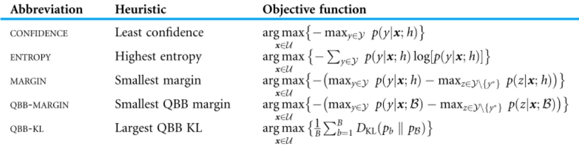
For convenience, we summarize the five heuristics discussed above inTable 1.
COMBINING SUGGESTIONS
Out of the five heuristics discussed, which one should we use in practice when we would like to apply active learning to a particular problem? There have been some attempts in the literature to do a theoretical analysis of their performance. Proofs are however scarce, and when there is one available, they normally only work under restrictive assumptions. For example,Freund et al. (1997)showed that the query by committee algorithm (a slight variant of our two QBB heuristics) guarantees an exponential decrease in the prediction error with the training size, but only when there is no noise. In general, whether any of these heuristics is guaranteed to beat passive learning is still an open question.
Even though we do not know which one is the best, we can still combine suggestions from all of the heuristics. This can be thought of as the problem of prediction with expert advice, where each expert is an active learning heuristic. In this paper we explore two different approaches: we can either consider the advice of only one expert at each time step (with bandit algorithms), or we can aggregate the advice of all the experts (with social choice theory).
Combining suggestions with bandit theory
First let us turn our attention to the multi-armed bandit problem in probability theory (Berry & Fristedt, 1985). The colorful name originates from the situation where a gambler
Table 1 Summary of active learning heuristics used in our experiments.
Abbreviation Heuristic Objective function
CONFIDENCE Least confidence arg max
x2U maxy2Y pðyjx;hÞ
ENTROPY Highest entropy arg max
x2U
Py2Y pðyjx;hÞlog½pðyjx;hÞ
MARGIN Smallest margin arg max
x2U maxy2Y pðyjx;hÞ maxz2Ynfy
g pðzjx;hÞ
QBB-MARGIN Smallest QBB margin arg max
x2U maxy2Y pðyjx;BÞ maxz2Ynfy
g pðzjx;BÞ
QBB-KL Largest QBB KL arg max
x2U 1 B PB b¼1DKLðpbkpBÞ Note:
Notations:p(y|x;h) is the probability of that an object with feature vectorxhas labelyunder classifierh,Bis the set ofB classifiers {h1,h2,: : :,hB},Yis the set of possible labels,yis the most certain label,Uis the set of unlabeled instances,
DKL(p||q) is the Kullback–Leibler divergence ofpfromq, andpBis the class distribution averaged across classifiers inB. For consistency, with heuristics that use minimization, we flip the sign of the score so that we can always take the argmax to get the best candidate.
stands in front of a slot machine withRlevers. When pulled, each lever gives out a reward according to some unknown distribution. The goal of the game is to come up with a strategy that can maximize the gambler’s lifetime rewards. In the context of active learning, each lever is a heuristic with a different ability to identify the candidate whose labeling information is most valuable.
The main problem in multi-armed bandits is the trade-off between exploring random heuristics and exploiting the best heuristic so far. There are many situations in which we find our previously held beliefs to be completely wrong. By always exploiting, we could miss out on the best heuristic. On the other hand, if we explore too much, it could take us a long time to reach the desired accuracy.
Bandit algorithms do not need to know the internal workings of the heuristics, but only the reward received from using any of them. At each time step, we receive a reward from a heuristic, and based on the history of all the rewards, the bandit algorithm can decide on which heuristic to pick next. Formally, we need to learn the function
b:ðJR ½0;1Þn!JR (15)
wherebis the bandit algorithm, the reward is normalized between 0 and 1,Jℛis the index
set over the set of heuristicsℛ, andnis the time horizon.
What would be an appropriate rewardwin this setting? We propose using the incremental increase in the performance of the test set after the candidate is added to the training set. This, of course, means that we need to keep a separate labeled test set around, just for the purpose of computing the rewards. We could, as is common practice in machine learning, use cross validation or bootstrap on ℒTto estimate the
generalization performance. However for simplicity of presentation we use a separate test setℒS.
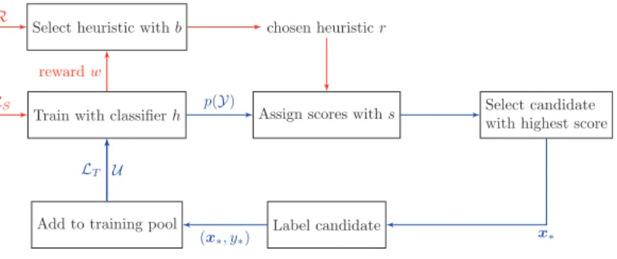
Figure 1andAlgorithm 2outline how bandits can be used in pool-based active learning. The only difference between the bandit algorithms lies in the SELECTfunction
that selects which heuristic to use, and the UPDATE function that updates the algorithm’s
selection parameters when receiving a new reward.
Train with classifierh Assign scores withs Select candidatewith highest score
Label candidate Add to training pool
Select heuristic withb chosen heuristicr
LT p(Y) x∗ (x∗, y∗) LS U rewardw R
Figure 1 Active learning pipeline with bandit algorithms.We need to collect rewardswfrom the test setℒSin order to decide which heuristic to choose at each time step. This routine is indicated by the red
arrows. Notations:ℛis the set of heuristics {r1, : : :,rR},ℒTis the training set,ℒSis the test set,Uis the
unlabeled set, andp(Y) is the predicted class probabilities on the unlabeled dataU.
There have been some attempts to combine active learning suggestions in the literature. Baram, El-Yaniv & Luz (2004)used the EXP4 multi-armed bandit algorithm to automate the selection process. They proposed a reward called the classification entropy
maximization, which can be shown to grow at a similar rate to the true accuracy in binary classification with support vector machines (SVMs). We will not compare our results directly with those in Baram, El-Yaniv & Luz (2004)since we would like to evaluate algorithms that can work with both binary and multi-class classification. Our experiments also use logistic regression which produces probability estimates directly, rather than SVMs which can only produce unnormalized scores. Hsu & Lin (2015) studied an improved version of EXP4, called EXP4.P, and used importance weighting to estimate the true classifier performance using only the training set. In this paper, we empirically compare the following four bandit algorithms: Thompson sampling, OC-UCB, kl-OC-UCB, and EXP3++.
Thompson sampling
The oldest bandit algorithm is Thompson sampling (Thompson, 1933) which solves the exploration-exploitation trade-off from a Bayesian perspective.
LetWibe the reward of heuristicri∈ℛ. Observe that even with the best heuristic, we
still might not score perfectly due to having a poor classifier trained on finite data. Conversely, a bad heuristic might be able to pick an informative candidate due to pure luck. Thus there is always a certain level of randomness in the reward received. Let us treat the reward Wi as a normally distributed random variable with meanνiand
variance t2
i:
ðWijiÞ N ði;t2iÞ (16)
If we knew bothνiandti2for all heuristics, the problem would become trivially
easy since we just need to always use the heuristic that has the highest mean
Algorithm 2 Pool-based active learning with bandit theory. Note that in addition to the set of active learning heuristicsℛand the test setℒS, some bandit algorithms also need to known, the maximum size of the training set, in advance.
Input:unlabeled setU, labeled training setℒT, labeled test setℒS, classifierh, desired training sizen, set of
active learning heuristicsℛ, and bandit algorithmbwith two functions SELECTand UPDATE. whilejℒTj<ndo
Select a heuristicr∈ℛaccording to SELECT.
Select the most informative candidatexfromUusing the chosen heuristicr(U;h).
Ask the expert to labelx. Call the labely.
Add the newly labeled example to the training set:LT LT[ fðx;yÞg. Remove the newly labeled example from the unlabeled set:U Unfxg. Retrain the classifierh(x) usingℒT.
Run the updated classifier on the test setℒSto compute the increase in the performancew.
Update the parameters ofbwith UPDATE(w). end
reward. In practice, we do not know the true mean of the rewardνi, so let us add a second layer of randomness and assume that the mean itself follows a normal distribution: i N ðmi;s2
iÞ (17)
To make the problem tractable, let us assume that the varianceti2in the first layer is
a known constant. The goal now is to find a good algorithm that can estimatemiandsi
2 . We start with a prior onmiandsi2for each heuristicri. The choice of prior does
not usually matter in the long run. Since initially we do not have any information about the performance of each heuristic, the appropriate prior value formiis 0, i.e., there
is no evidence (yet) that any of the heuristics offers an improvement to the performance. In each round, we draw a random sampleνi′from the normal distributionN ðmi;s2iÞ for eachiand select heuristic r that has the highest sampled value of the mean reward:
r¼arg max
i
vi0 (18)
We then use this heuristic to select the object that is deemed to be the most informative, add it to the training set, and retrain the classifier. Next we use the updated classifier to predict the labels of objects in the test set. Letwbe the reward observed. We now have a new piece of information that we can use to update our prior belief about the meanm
and the variances2of the mean reward. Using Bayes’ theorem, we can show that the
posterior distribution of the mean reward remains normal,
ðjW¼wÞ N ðm0; s02Þ (19)
with the following new mean and variance: m0 ¼ mt2 þws2 s2 þt2 s02 ¼ s2 t2 s2 þt2 (20) Algorithm 3summarizes the SELECTand UPDATEfunctions used in Thompson sampling. Upper confidence bounds
Next we consider the Upper Confidence Bound (UCB) algorithms which use the principle of “optimism in the face of uncertainty.” In choosing which heuristic to use, we first estimate the upper bound of the reward (that is, we make an optimistic guess) and pick
Algorithm 3 Thompson sampling with normally distributed rewards. Notations:ℛis the set of
Rheuristics,mis the mean parameter of the average reward,s2is the variance parameter of the average reward,t2 is the known variance parameter of the reward, andw is the actual reward received.
functionSELECT()
fori∈{1, 2, ...,R}do
νi′draw a sample fromN ðmi;s2iÞ
end
Select the heuristic with the highest sampled value:r argmax
i 0 i functionUPDATE(w) m mt 2 þws2 s2 þt2 s2 s2 t2 s2 þt2
the one with the highest bound. If our guess turns out to be wrong, the upper bound of the chosen heuristic will decrease, making it less likely to get selected in the next iteration. There are many different algorithms in the UCB family, e.g., UCB1-TUNED & UCB2 (Auer, Cesa-Bianchi & Fischer, 2002a), V-UCB (Audibert, Munos & Szepesva´ri, 2009), OC-UCB (Lattimore, 2015), and kl-UCB (Cappe´ et al., 2013). They differ only in the way the upper bound is calculated. In this paper, we only consider the last two. In Optimally Confident UCB (OC-UCB),Lattimore (2015)suggests that we pick the heuristic that maximizes the following upper bound:
r¼arg max i wiþ ffiffiffiffiffiffiffiffiffiffiffiffiffiffiffiffiffiffiffiffiffiffiffiffiffiffiffi a TiðtÞ ln cn t s ! (21) wherewi is the average of the rewards fromrithat we have observed so far,tis the time
step,Ti(t) is the number times we have selected heuristic ri before stept, andnis the
maximum number of steps that we are going to take. There are two tunable parameters, a andc, which the author suggests setting to 3 and 2, respectively.
In kl-UCB,Cappe´ et al. (2013)suggest that we can instead consider the KL-divergence between the distribution of the current estimated reward and that of the upper bound. In the case of normally distributed rewards with known variances2, the chosen heuristic would be r¼arg max i wiþ ffiffiffiffiffiffiffiffiffiffiffiffiffiffiffiffiffiffiffiffiffiffiffiffiffiffi 2s2lnðTiðtÞÞ t r ! (22) Algorithms 4and5summarize these two UCB approaches. Note that the size of the rewardwis not used in UPDATE(w) of UCB, except to select the best arm.
Algorithm 4 Optimally Confident UCB. Notations:nis the time horizon (maximum number of time steps),tis the current time step,Ti(t) counts how many times heuristicihas been selected before
stept,wis the reward received, andwiis the average of the rewards fromriso far.
fuctionSELECT() r arg max i wiþ ffiffiffiffiffiffiffiffiffiffiffiffiffiffiffiffiffiffiffiffiffiffiffiffiffiffiffiffi 3 TiðtÞ ln 2n t r functionUPDATE(w) t tþ1 TðtÞ Tðt1Þ þ1
Algorithm 5 kl-UCB with normally distributed rewards. Notations: s2 is the variance of the rewards, t is the current time step, Ti(t) counts how many times heuristic i has been selected
before stept,wis the reward received, andwiis the average of the rewards fromriso far.
functionSELECT() r arg max i wiþ ffiffiffiffiffiffiffiffiffiffiffiffiffiffiffiffiffiffiffiffiffiffiffiffiffiffi 2s2lnðTiðtÞÞ t r functionUPDATE(w) t tþ1 TðtÞ Tðt1Þ þ1
EXP3++
The exponential-weight algorithm for exploration and exploitation (EXP3) was first developed byAuer et al. (2002b) to solve the non-stochastic bandit problem where we make no statistical assumptions about the reward distribution. This is also often known as the adversarial setting, where we have an adversary who generates an arbitrary sequence of rewards for each heuristic in advance. Like Thompson sampling, the algorithm samples from a probability distribution at each step to pick a heuristic. Here however, we construct the distribution with exponential weighting (hence the name EXP3). We shall test Seldin & Slivkins (2014)’s EXP3++ algorithm (seeAlgorithm 6). This is a generalization of the original EXP3 and it has been shown to perform well in both the stochastic (where the reward of each heuristic follows an unknown reward distribution) and the adversarial regime.
Combining suggestions with social choice theory
A drawback of the above bandit methods is that at each iteration, we could only use one suggestion from one particular heuristic. EXP4 and EXP4.P algorithms can take advice from all heuristics by maintaining a weight on each of them. However, being a bandit method, they require designing a reward scheme. If the reward is the performance on a test set, we would need to keep around a separate subset of the data, which is expensive and sometimes impossible to obtain in practice. This leads us to social choice theory, which can combine suggestions like EXP4 and EXP4.P, while not needing the concept of a reward. Originally developed by political scientists like Nicolas de Condorcet and Jean-Charles de Borda, this field of study is concerned with how we aggregate preferences of a group of people to determine, for example, the winner in an election
Algorithm 6 EXP3++ algorithm. Notations:ℛis the set ofRheuristics,tis the current time step,bis a parameter used to weight the heuristics for selection,ξiandεiare used to compute the lossLi,ρis
the distribution from which a heuristic is sampled, andwis the reward received. functionSELECT() b¼1 2 ffiffiffiffiffiffiffiffi lnR tR r fori∈{1, 2, ...,R}do ji¼ 18 InðtÞ2 tminð1;1 tðLiminðLÞÞÞ 2 εi¼min 1 2R;b;ji ri¼ ebLi P jebLj end
r draw a sample fromℛwith probability distributionρ. functionUPDATE(w)
t tþ1
TðtÞ Tðt1Þ þ1
L Lþ ð1wÞ
(List, 2013). It has the nice property that everyone (or in our context, every active learning heuristic) has a voice.
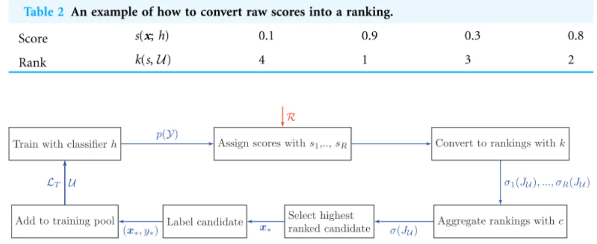
For each heuristic, we assign a score to every candidate with the score functions(x,h) like before. We are neither interested in the actual raw scores nor the candidate with the highest score. Instead, we only need a ranking of the candidates, which is achieved by a function kðs;UÞthat provides a ranking of the unlabeled examples according to their scores. For example,kcould assign the candidate with the highest score a rank of 1, the next best candidate a rank of 2, and so on. An aggregation functioncwill then combine all the rankings into a combined ranking,
c:sðJUÞR !sðJUÞ (23)
wheresðJUÞis a permutation over the index set of the unlabeled poolU andRis the
number of heuristics. From these we can pick the highest-ranked candidate to annotate. SeeTable 2for an example.
The main difference between this approach and the bandit algorithms is that we do not consider the reward history when combining the rankings. Here each heuristic is assumed to always have an equal weight. A possible extension, which is not considered in this paper, is to use the past performance to re-weight the heuristics before aggregating at each step.Figure 2andAlgorithm 7 provide an overview of how social choice theory is used in pool-based active learning.
The central question in social choice theory is how we can come up with a good preference aggregation rule. We shall examine three aggregation rules: Borda count, the geometric mean, and the Schulze method.
In the simplest approach, Borda count, we assign an integer point to each candidate. The lowest-ranked candidate receives a point of 1, and each candidate receives one more point than the candidate below. To aggregate, we simply add up all the points each
Table 2 An example of how to convert raw scores into a ranking.
Score s(x;h) 0.1 0.9 0.3 0.8
Rank k(s,U) 4 1 3 2
Train with classifierh Assign scores withs1,..,sR Convert to rankings withk
Aggregate rankings withc
Select highest ranked candidate Add to training pool Label candidate
LT U p(Y) σ1(JU), ..., σR(JU) σ(JU) x∗ (x∗, y∗) R
Figure 2 Active learning pipeline with rank aggregation methods.Unlike the bandit pipeline, there is only one cycle in which we aggregate information from all heuristics. Additional notation:sðJUÞis a permutation (i.e., rank) on the index set of the unlabeled data.
candidate receives from every heuristic. The candidate with the most points is declared the winner and is to be labeled next. We can think of Borda count, then, as ranking the candidate according to the arithmetic mean.
An alternative approach is to use the geometric mean, where instead of adding up the points, we multiply them. Bedo¨ & Ong (2016)showed that the geometric mean maximizes the Spearman correlation between the ranks. Note that this method requires the ranks to be scaled so that they lie strictly between 0 and 1. This can be achieved by simply dividing the ranks by (U+ 1), whereUis the number of candidates.
The third approach we consider is the Schulze method (Schulze, 2011). Out of the three methods considered, this is the only one that fulfills the Condorcet criterion, i.e., the winner chosen by the algorithm is also the winner when compared individually with each of the other candidates. However, the Schulze method is more computationally intensive since it requires examining all pairs of candidates. First we compute the number of heuristics that prefer candidatexito candidatexj, for all possible pairs (xi,xj). Let us
call this d(xi,xj). Let us also define a path from candidate xi toxjas the sequence of
candidates, {xi,x1,x2, ...,xj}, that starts withxi and ends withxj, where, as we move
along the path, the number of heuristics that prefer the current candidate over the next candidate must be strictly decreasing. Intuitively, the path is the rank of a subset of candidates, wherexiis the highest-ranked candidate andxjis at the lowest-ranked.
Associated with each path is a strengthp, which is the minimum ofd(xi, xj) for all
consecutive xiandxjalong the path. The core part of the algorithm involves finding
the path of the maximal strength from each candidate to every other. Let us callp(xi,xj)
the strength of strongest path betweenxiandxj. Candidatexiis a potential winner if
pðxi;xjÞ pðxj;xiÞfor all otherxj. This problem has a similar flavor to the problem of
finding the shortest path. In fact, the implementation uses a variant of the Floyd–Warshall algorithm to find the strongest path. This is the most efficient implementation that we know of, taking cubic time in the number of candidates.
Algorithm 7 Pool-based active learning with social choice theory.
Input:unlabeled setU, labeled training setℒT, classifierh, set of active learning suggestionsR, ranking
functionk, and rank aggregatorc. repeat:
forr∈Rdo
Rank all the candidates inUwithk. end
Aggregate all the rankings into one ranking using the aggregatorc. Select the highest-ranked candidatexfromU.
Ask the expert to labelx. Call the labely.
Add the newly labeled example to the training set:LT LT[ fðx;yÞg.
Remove the newly labeled example from the unlabeled set:U Unfxg. Retrain the classifierh(x) usingℒT.
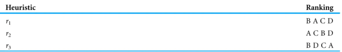
We end this section with a small illustration of how the three aggregation algorithms work inTable 3.
EXPERIMENTAL PROTOCOL
We use 11 classification datasets taken from the UCI Machine Learning Repository (https://archive.ics.uci.edu/ml/) (Lichman, 2013), with a large multiclass classification dataset which we extracted from the SDSS project (DOI 10.5281/zenodo.58500) (Alam et al., 2015). The code for the experiments can be found on our GitHub repository (https://github.com/chengsoonong/mclass-sky).Table 4shows the size and the number of classes in each dataset, along with the proportion of the samples belonging to the majority class and the maximum achievable performance using logistic regression. These datasets were chosen such that we have an equal number of binary and multiclass datasets, and a mixture of small and large datasets.
For each dataset, we use Scikit-learn (Pedregosa et al., 2011) to train a logistic regression model using a 10-fold stratified shuffled cross-validation. Here “stratified” means that the proportion of the classes remains constant in each split. We standardize all features to have zero mean and unit variance. Although all examples have already been labeled, Table 3 An example of how social choice theory algorithms rank candidates by aggregating three heuristics:r1,r2, andr3.There are four candidates in the unlabeled pool: A, B, C, and D.
(a) An example of how the three heuristics rank four candidatesA,B,C, andD. For instance, heuristic
r1considersBto be the highest rank candidate, followed byA,C, andD.
Heuristic Ranking
r1 B A C D
r2 A C B D
r3 B D C A
(b) Aggregated ranking with Borda count and geometric mean. The scores are determined by the relative ranking in each heuristic. For example,Ais ranked second byr1, first byr1, and last byr3, thus
giving us a score of 3, 4, and 1, respectively. In both methods, candidateBreceives the highest aggregated score.
Candidate Borda count Geometric mean
A 3 + 4 + 1 = 8 341 = 12
B 4 + 2 + 4 = 10 424 = 32
C 2 + 3 + 2 = 7 232 = 12
D 1 + 1 + 3 = 5 113 = 3
(c) Aggregated ranking with the Schulze method. The table shows the strongest path strengthp(xi,xj)
between all pairs of candidates. For example,p(B,D) = 3 because the pathB/Dis the strongest path fromBtoD, where three heuristics preferBoverD. CandidateBis the winner sincep(B,A) >p(A,B),
p(B, C)> p(C, B), andp(B,D) >p(D,B). From/To A B C D A – 1 2 2 B 2 – 2 3 C 1 1 – 2 D 2 0 1 –
we simulate the active learning task by assuming that certain examples do not have any labels. For each fold, the unlabeled pool size is 70% of data up to a maximum of 10,000 examples, and the test pool consists of the remaining examples up to a maximum of 20,000. We assume all test examples are labeled. We initialize the classifier by labeling 10 random instances and using them as the initial training set. The heuristics are fast enough such that we can assign a score to every unlabeled instance at every time step. We use logistic regression with a Gaussian kernel approximation and an L2 regularizer. In the binary case, the loss function is
L¼1 2θ
TθþCX n
i¼1
ln 1 þexpðyiðθTfðxiÞÞÞ (24)
wherexiis the feature vector of theith example,yi∈{0, 1} is the label ofxi, andnis
the training size. The term1 2θ
Tθis the regularization term to ensure that the weight vector θis not too large, andCis a regularization hyperparameter in [10-6, 106] which we find using grid search. To speed up the training time while using the Gaussian kernel, we approximate the feature map of the kernel with Random Kitchen Sinks (Rahimi & Recht, 2008), transforming the raw featuresxiinto a fixed 100-dimensional feature vectorf(xi).
In the multiclass case, we use the One-vs-Rest strategy, where for every class we build a binary classifier that determines whether a particular example belongs to that class or not. For the QBB algorithms, we train a committee of seven classifiers, where each member is given a sample of maximum 100 examples that have already been labeled.
For the bandit algorithms, we use the increase in the MPBA on the test set as the reward. The MPBA can be thought of as the expected value of the average recall, where
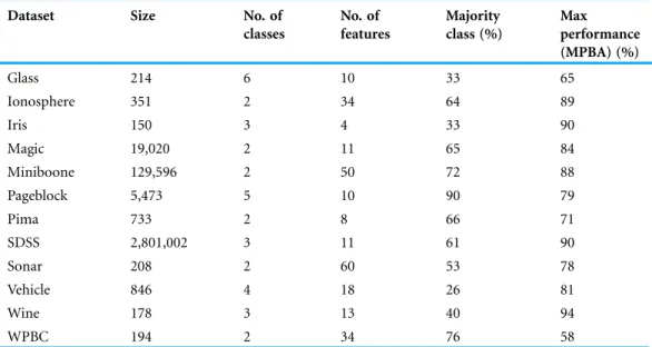
Table 4 Overview of datasets.
Dataset Size No. of
classes No. of features Majority class (%) Max performance (MPBA) (%) Glass 214 6 10 33 65 Ionosphere 351 2 34 64 89 Iris 150 3 4 33 90 Magic 19,020 2 11 65 84 Miniboone 129,596 2 50 72 88 Pageblock 5,473 5 10 90 79 Pima 733 2 8 66 71 SDSS 2,801,002 3 11 61 90 Sonar 208 2 60 53 78 Vehicle 846 4 18 26 81 Wine 178 3 13 40 94 WPBC 194 2 34 76 58 Note:
The following datasets are from the UCI Machine Learning Repository: glass, ionosphere, iris, magic, miniboone, pageblock, pima, sonar, vehicle, wine, and wpbc. In particular, the vehicle dataset comes from the Turing Institute, Glasgow, Scotland. The sdss dataset was extracted from Data Release 12 of SDSS-III.
we treat the recall as a random variable that follows a Beta distribution. Compared to the raw accuracy score, this metric takes into account class imbalance. This is because we first calculate the recall in each class and then take the average, thus giving each class an equal weight. Refer to Appendix A for the derivation of the MPBA, which extendsBrodersen et al. (2010)’s formula from the binary to the multiclass setting.
In total, we test 17 query strategies. This includes passive learning, eight active learning heuristics, five bandit algorithms, and three aggregation methods. The bandit algorithms include the four described in “Combining Suggestions with Bandit Theory” and a baseline calledEXPLOREwhich simply selects a random heuristic at each time step.
In other words, we ignore the rewards and explore 100% of the time. For all bandit and rank aggregation methods, we take advice from six representative experts: PASSIVE, CONFIDENCE,MARGIN,ENTROPY,QBB-MARGIN, andQBB-KL. We have not explored how adding
the heuristics with information density weighting to the bandits would impact the performance. See Table 5for a list of abbreviations associated with the methods.
Given that there are 12 datasets, each with 17 learning curves, we need a measure that can summarize in one number how well a particular heuristic or policy does. Building onBaram, El-Yaniv & Luz (2004)’s deficiency measure, we define the strength of an active learner or a combiner relative to passive learning as
Strengthðh;mÞ ¼1 Pn t¼1ðmðmaxÞ mðh;tÞÞ Pn t¼1ðmðmaxÞ mðpassive;tÞÞ (25) wheremis a chosen metric (e.g., accuracy rate, MPBA), m(max) is the best possible performance1, andm(h,t) is the performance achieved using the firsttexamples selected by
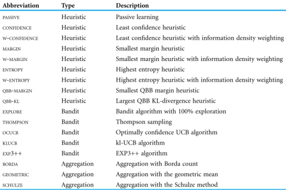
Table 5 Summary of active learning heuristics and combiners used in the experiments.
Abbreviation Type Description
PASSIVE Heuristic Passive learning
CONFIDENCE Heuristic Least confidence heuristic
W-CONFIDENCE Heuristic Least confidence heuristic with information density weighting MARGIN Heuristic Smallest margin heuristic
W-MARGIN Heuristic Smallest margin heuristic with information density weighting ENTROPY Heuristic Highest entropy heuristic
W-ENTROPY Heuristic Highest entropy heuristic with information density weighting QBB-MARGIN Heuristic Smallest QBB margin heuristic
QBB-KL Heuristic Largest QBB KL-divergence heuristic EXPLORE Bandit Bandit algorithm with 100% exploration THOMPSON Bandit Thompson sampling
OCUCB Bandit Optimally confidence UCB algorithm KLUCB Bandit kl-UCB algorithm
EXP3++ Bandit EXP3++ algorithm
BORDA Aggregation Aggregation with Borda count GEOMETRIC Aggregation Aggregation with the geometric mean SCHULZE Aggregation Aggregation with the Schulze method
1The best possible performance in each
trial is obtained by the higher of: (1) the performance achieved by using all the labeled examples in the training set; and (2) the maximum value of the learning curves of all the methods.
heuristich. We can think of the summation as the area between the best possible performance line and the learning curve of h. The better the heuristic is, the faster it would approach this maximum line, and thus the smaller the area. Finally, so that we can compare the performance across datasets, we normalize the measure with the area obtained from using just passive learning. Refer to Fig. 3for a visualization of the strength measure.
We evaluate the algorithm performance with two metrics: the accuracy score and the MPBA. The accuracy score is the percentage of instances in the test set where the predicted label matches the true label. If a dataset has a dominant class, then the accuracy score of instances within that class will also dominate the overall accuracy score. The MPBA, on the other hand, puts an equal weight on each class and thus favors algorithms that can predict the label of all classes equally well.
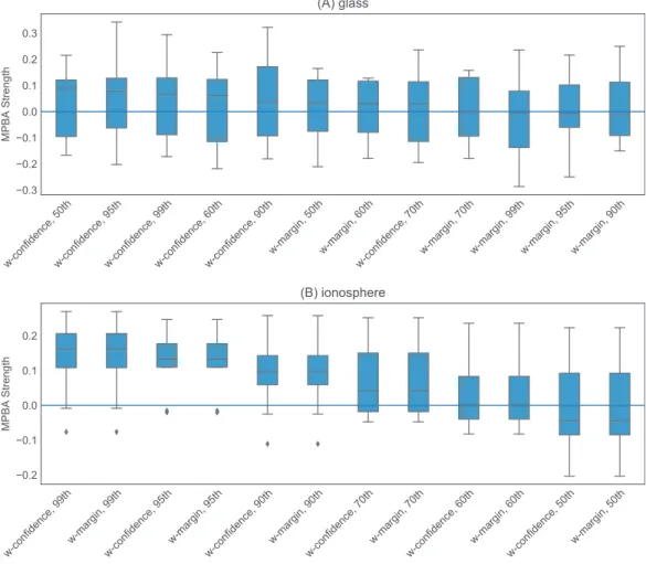
The heuristics with information density weighting and Thompson sampling have a few additional hyperparameters. To investigate the effect of these hyperparameters, we pick one binary dataset (glass) and one multiclass dataset (ionosphere) to investigate. Both of these are small enough to allow us to iterate through many hyperparameter values quickly. With W-CONFIDENCE,W-MARGIN, andW-ENTROPY, we setgin the Gaussian kernel
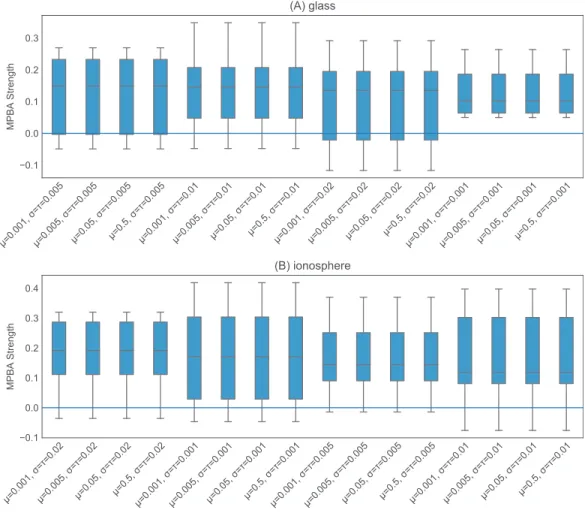
to be the inverse of the 95th percentile of all pairwise distances. This appears to work well, as shown in Fig. 4. ForTHOMPSON, the prior values form,s2and the value oft2seem
to have little effect on the final performance (seeFig. 5). We set the initialmto 0.5, the initials2to 0.02, andt2to 0.02.
RESULTS
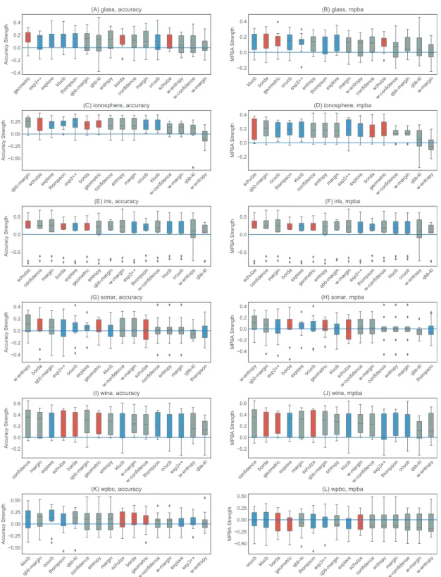
Figures 6and7show the strengths of all methods that we consider, while Figs. 8and9 provide selected learning curves. Plots for the six small datasets with fewer than 500
Figure 3 An illustration of the MPBA strength measure.It is proportional to the shaded area between the (red) passive learning curve and the (blue) active learning curve. The bigger the area is, the more the active learner outperforms the passive learner. The top dotted line indicates the maximum performance
examples (glass, ionosphere, iris, sonar, wine, and wpbc) are shown inFigs. 6and8. Plots for the two medium-sized datasets (pima and vehicle) and the four large datasets (magic, miniboone, pageblocks, and sdss) are shown in Figs. 7and9. Each figure contains two subfigures, one reporting the raw accuracy score, while the other showing the MPBA score.
Active learning methods generally beat passive learning in four of the six small datasets— glass, ionosphere, iris, and wine. This can be seen by the fact that the boxplots are mostly above the zero line inFig. 6. For sonar and wpbc, the results are mixed—active learning has little to no effect here. The wpbc dataset is particularly noisy—our classifier cannot achieve an MPBA score greater than 60% (seeFig. 8). Thus it is not surprising that active learning does not perform well here since there is not much to learn to begin with.
The advantage of active learning becomes more apparent with the larger datasets like magic, miniboone, pageblocks, and sdss. Here there is a visible gap between the
Figure 4 Effect ofg onW-CONFIDENCEand W-MARGINusing the glass and ionosphere datasets.We examine six different values forg: the 50th, 60th, 70th, 90th, 95th, and 99th percentile of the pairwise L1-distance between the data points. For the glass dataset (A), changing value ofghas minimal effect on the results, while for the ionosphere dataset (B), using the 90th percentile and above seems to work well.
passive learning curve and the active learning curve for most methods. For instance, using a simple heuristic such asCONFIDENCEin the pageblocks dataset results in an average
MPBA score of 74% after 1,000 examples, while passive learning can only achieves 67% (seeFig. 9F).
Out of the eight active learning heuristics tested, the heuristics with the
information density weighting (W-CONFIDENCE,W-MARGIN, and W-ENTROPY) generally
perform worse than the ones without the weighting.QBB-KLperforms the best in
pageblocks while it can barely beat passive learning in other datasets. The remaining heuristics—CONFIDENCE, MARGIN,ENTROPY, andQBB-MARGIN—perform equally well in
all datasets.
We find no difference in performance between the bandit algorithms and the rank aggregation methods. Combining active learners does not seem to hurt the performance, even if we include a poorly performing heuristic such asQBB-KL.
For bandit algorithms, it is interesting to note thatTHOMPSONfavors certain heuristics a
lot more than others, while the behavior ofEXP3++,OCUCB, andKLUCBis almost
Figure 5 Effect of the initial values of the parameters inTHOMPSON.We test 16 combinations ofm,s2,
andt2on the glass (A) and ionosphere (B) dataset. Varying these values does not seem to affect the final
Figure 6 Boxplots of the accuracy and MPBA strength of the 16 active learning strategies, relative to passive learning, using the small datasets (glass, ionosphere, iris, sonar, wine, and wpbc).The more positive the strength is, the better the heuristic/combiner is. Gray boxes represent individual heuristics; blue boxes represent bandit algorithms, and red boxes are for rank aggregation methods. A strategy that is above the zero line is better than passive learning. Each boxplot contains 10 trials. The accuracy score (A, C, E, G, I, and K) is a simple metric that simply counts up the number of correct predictions. The MPBA score (B, D, F, H, J, and L), being the weighted average of the recall and precision, gives an equal representation to each class. The boxes represent the quartiles and the whiskers extend to 1.5 times of the interquartile range.
Figure 7 Boxplots of the accuracy and MPBA strength of the 16 active learning strategies, relative to passive learning, using medium to the large datasets (magic, miniboone, pageblocks, pima, sdss, and vehicle).The more positive the strength is, the better the heuristic/combiner is. Gray boxes represent individual heuristics; blue boxes represent bandit algorithms, and red boxes are for rank aggregation methods. A strategy that is above the zero line is better than passive learning. Each boxplot contains 10 trials. The accuracy score (A, C, E, G, I, and K) is a simple metric that simply counts up the number of correct predictions. The MPBA score (B, D, F, H, J, and L), being the weighted average of the recall and precision, gives an equal representation to each class. The boxes represent the quartiles and the whiskers extend to 1.5 times of the interquartile range.
Figure 8 Selected accuracy and MPBA learning curves for the small datasets (glass, ionosphere, iris, sonar, wine, and wpbc).As it would get too cluttered to plot 17 learning curves, we only show the accuracy (A, C, E, G, I, and K) and MPBA (B, D, F, H, J, and L) learning curves forPASSIVE, CONFIDENCE,EXP3++, andBORDA. The learning curves are averaged over 10 trials. The dotted horizontal line shows the performance obtained from
Figure 9 Selected accuracy and MPBA learning curves for the medium to large datasets (magic, miniboone, pageblocks, pima, sdss, and vehicle).As it would get too cluttered to plot 17 learning curves, we only show the accuracy (A, C, E, G, I, and K) and MPBA (B, D, F, H, J, and K) learning curve forPASSIVE,CONFIDENCE,EXP3++, andBORDA. The learning curves are averaged over 10 trials. The dotted horizontal line shows the performance obtained from using the whole training data. Full-size DOI: 10.7717/peerj-cs.157/fig-9
Figure 10 Selection frequencies of heuristics inTHOMPSONandEXP3++, with the large datasets (magic, miniboone, pageblocks, pima, sdss, and vehicle).The plots show how often each of the heuristics gets selected over time. The selection frequencies are averaged over 10 trials.THOMPSON (A–F) favors certain heuristics more strongly than others. In contrast,EXP3++ (G–L) favors uniform exploration more, sampling each heuristic with roughly equal weights. The plots forOCUCBandKLUCBare not shown here, but they are similar toEXP3++.
Figure 11 The effect of the initial values of the parameters inTHOMPSONon the heuristic selection frequencies.We test 16 combinations ofm,s2, andt2on the glass and ionosphere dataset. Which heuristicsTHOMPSONpicks seems to correlate with the heuristic performance. For example, in
ionosphere,PASSIVE(the dotted purple line) andQBB-KL(the dashed dark blue line) tend to get picked less often than others.
indistinguishable from EXPLORE, where we explore 100% of the time (seeFig. 10).
Changing the initial values ofm,s2, andt2changes the order of preference slightly, but overall, which heuristicsTHOMPSONpicks seems to correlate with the heuristic
performance. For example, as shown in Fig. 11,PASSIVEandQBB-KLtend to get chosen
less often than others in the ionosphere dataset.
DISCUSSION
The experimental results allow us to answer the following questions:
1.Can active learning beat passive learning?Yes, active learning can perform much better than passive learning, especially when the unlabeled pool is large (e.g., sdss, miniboone, pageblock). When the unlabeled pool is small, the effect of active learning becomes less apparent, as there are now fewer candidates to choose from. This can be seen inFig. 12, where we show that artificially reducing the unlabeled pool results in a reduction in the final performance. At the same time, having a small test set also makes the gap between the active learning curve and the passive learning curve smaller (seeFigs. 12Cand12F). This further contributes to the poorer performance on the smaller datasets. In any case, when a dataset is small, we can label everything so active learning is usually not needed.
Figure 12 Effect of the pool size on the learning curves. We pick two large datasets—pageblocks and sdss—to investigate how the size of the pool affects the performance.(A) and (D) are the original learning curves fromFigs. 9Fand9J(we only show the first 200 examples so that all figures have the same scale). For (B) and (E), we use the same test pool, but the unlabeled pool now only has a maximum of 300 candidates. Finally, for (C) and (F) the combined test pool and training pool have a size of 300.
2.Can active learning degrade performance?Yes, there is no guarantee that active learning will always beat passive learning. For example,W-ENTROPYactually slows down
the learning in the many datasets. However, this only happens with certain heuristics, like those using the information density weighting.
3.What is the best single active learning heuristic?All ofCONFIDENCE,MARGIN,ENTROPY,
andQBB-MARGINhave a similar performance. However CONFIDENCEis perhaps the
simplest to compute and thus is a good default choice in practice. 4.What are the challenges in using bandit algorithms?
(a) Designing a good reward scheme is difficult. This paper uses the increase in the classifier performance as the reward. However this type of reward is non-stationary (i.e., it gets smaller after each step as learning saturates) and the rewards will thus eventually go to zero.
(b) In practice, we do not have a representative test set that can be used to compute the reward. As a workaround,Hsu & Lin (2015)computed the reward on the training set and then used importance weighting to remove any potential bias. For this to work, we need to ensure that every training example and every active learning suggestion have a non-zero probability of being selected in each step.
(c) Finally, some bandit algorithms such as Thompson sampling assumes that the reward follows a certain distribution (e.g., Gaussian). However, this assumption is unrealistic.
5.What are the challenges in using rank aggregation algorithms?
(a) We need to compute the scores from all heuristics at every time step. This might not be feasible if there are too many heuristics or if we include heuristics that require a large amount of compute power (e.g., variance minimization). (b) The Schulze method usesO(n2) space, wherenis the number of candidates.
This might lead to memory issues if we need to rank a large number of candidates from the unlabeled pool.
(c) Before aggregating the rankings, we throw away the score magnitudes, which could cause a loss of information.
(d) Unlike bandit algorithms, all of the rank aggregators always give each heuristic an equal weight.
6.Which method should I use in practice to combine active learners?Since there is no difference in performance between various combiners, we recommend using a simple rank aggregator like Borda count or geometric mean if we do not want to select a heuristic a priori. Rank aggregators do not need a notion of a reward—we simply give all suggestions an equal weight when combining. Thus we neither need to a keep a separate test set, nor do we need to worry about designing a good reward scheme.
Our investigation has a few limitations. Firstly, we empirically compare algorithms that only work with single-label classification problems. Nowadays, many problems require multi-label learning, in which each example is allowed to be in more than one class. Our methods can be extended to work with multi-label datasets with the following modifications. We first need a multi-label classifier. This can be as simple as a
collection of binary classifiers, each of which produces the probability that an example belongs to a particular class. For each class, we can use an active learning heuristic to assign a score to each unlabeled example as before. However now we need to aggregate the scores among the classes. As suggested byReyes, Morell & Ventura (2018), we can use any aggregation method like Borda count to combine these scores. In effect, the multi-label learning problem adds an extra layer of aggregation into the pipeline.
Another limitation of our methods is that our active learning methods are myopic. That is, in each iteration, we only pick one instance to give to a human expert for labeling. In many practical applications like astronomy, batch-mode active learning is preferred, as it is much more cost efficient to obtain multiple labels simultaneously. One naive extension is to simply choose themhighest ranked objects using our current methods. However, it is possible to have two unlabeled objects whose class membership we are currently uncertain about, but because they have very similar feature vectors, labeling only one of them would allow us to predict the label of the other one easily. More sophisticated batch-mode active learning approaches have been proposed to take into account other factors such as the diversity of a batch and the representativeness of each batch example. These approaches include looking at the angles between hyperplanes in support vector machines (Brinker, 2003), using cluster analysis (Xu, Akella & Zhang, 2007), and using an evolutionary algorithm (Reyes & Ventura, 2018). How to aggregate suggestions from these approaches is an interesting problem for future work.
CONCLUSION
In this paper we compared 16 active learning methods with passive learning. Our three main findings are: active learning is better than passive learning; combining active learners does not in general degrade the performance; and social choice theory provides more practical algorithms than bandit theory since we do not need to design a
reward scheme.
APPENDIX A: POSTERIOR BALANCED ACCURACY
Most real-world datasets are unbalanced. In the SDSS dataset, for example, there are 4.5 times as many galaxies as quasars. The problem of class imbalance is even more severe in the pageblocks dataset, where one class makes up 90% of the data and the remaining four classes only make up 10%. An easy fix is to under sample the dominant class when creating the training and test sets. This, of course, means that the size of these sets are limited by the size of the minority class.
When we do not want to alter the underlying class distribution or when larger training and test sets are desired, we need a performance measure that can correct for the class imbalance.Brodersen et al. (2010) show that the posterior balanced accuracy
distribution can overcome the bias in the binary case. We now extend this idea to the multi-class setting.
Suppose we havekclasses. For each classibetween 1 andk, there areNiobjects in the
universe. Given a classifier, we can predict the label of every object and compare our prediction with the true label. LetGibe the number of objects in classithat are correctly
predicted. Then we define the recallAiof classi as
Ai ¼ Gi Ni
(26) The problem is that it is not feasible to get the actual values ofGiandNisince that would
require us to obtain the true label of every object in the universe. Thus we need a method to estimate these quantities when we only have a sample. Initially we have no information aboutGiandNi, so we can assume that eachAifollows a uniform prior distribution
between 0 and 1. This is the same as a Beta distribution with shape parametersa=b= 1:
Ai Betað1;1Þ (27)
The probability density function (PDF) ofAi is then
fAiðaÞ ¼ ðaþbÞ ðaÞðbÞaa1ð1aÞ b1 /a11ð1aÞ11 (28)
whereC(a) is the gamma function.
After we have trained the classifier, suppose we have a test set containing niobjects
in classi. Running the classifier on this test set is the same as conductingkbinomial experiments, where, in theith experiment, the sample size is niand the probability
of success is simplyAi. Letgibe the number of correctly labeled objects belonging to classi
in the test set. Then, conditional on the recall rateAi,gifollows a binomial distribution:
ðgijAiÞ Binðni;AiÞ (29)
The probability mass function ofðgijAi ¼aÞ is thus pgijAiðgiÞ ¼ ni gi a gið1aÞnigi /agið1aÞnigi (30) In the Bayesian setting,Eq. (28)is the prior andEq. (30) is the likelihood. To get the posterior PDF, we simply multiply the prior with the likelihood:
fAijgðaÞ /fAiðaÞ fgijAiðgiÞ
/a11ð1aÞ11agið1aÞnigi
¼a1þgi1ð1aÞ1þnigi1
Thus, with respect to the binomial likelihood function, the Beta distribution is conjugate to itself. The posterior recall rateAialso follows a Beta distribution, now with parameters
ðAijgiÞ Betað1þgi;1þnigiÞ (32)
Our goal is to have a balanced accuracy rate,A, that puts an equal weight in each class. One way to achieve this is to take the average of the individual recalls:
A¼1 k Xk i¼1 Ai ¼1 kAT (33)
Here we have definedAT to be the sum of the individual recalls. We callðAjgÞthe
posterior balanced accuracy, where g= (g1, ...,gk). Most of the time, we simply want to
calculate its expected value:
E½Ajg ¼1 kE½ATjg ¼1 k Z afATjgðaÞda (34)
Let us call this the MPBA. Note that there is no closed form solution for the PDFfATjgðaÞ. However assuming thatATis a sum ofkindependent Beta random variables,fATjgðaÞcan be approximated by numerically convolving kBeta distributions. The independence
assumption is reasonable here, since there should be little to no correlation between the individual recall rates. For example, knowing that a classifier is really good at recognizing stars does not tell us much about how well that classifier can recognize galaxies.
Having the knowledge of fA|g(a) will allow us to make violin plots, construct confidence intervals and do hypothesis tests. To get an expression for this, let us first rewrite the cumulative distribution function as
FAjgðaÞ ¼PðAajgÞ ¼P 1 kAT ajg ¼PðAT kajgÞ ¼PFATjgðkaÞ (35)
Differentiating (Eq. (35)) with respect toa, we obtain the PDF of (A|g): fAjgðaÞ ¼ @ @aFAjgðkaÞ ¼ @ @aðkaÞ @ @kaFATjgðkaÞ ¼kfATjgðkaÞ (36)
A Python implementation for the posterior balanced accuracy can be found on our GitHub repository (https://github.com/chengsoonong/mclass-sky).
ADDITIONAL INFORMATION AND DECLARATIONS
Funding
The research was supported by the Data to Decisions Cooperative Research Centre whose activities are funded by the Australian Commonwealth Government’s Cooperative Research Centres Programme. This research was supported by the Australian Research Council Centre of Excellence for All-sky Astrophysics (CAASTRO), through project number CE110001020. The SDSS dataset was extracted from Data Release 12 of SDSS-III. Funding for SDSS-III has been provided by the Alfred P. Sloan Foundation, the Participating Institutions, the National Science Foundation, and the U.S. Department of Energy Office of Science. The SDSS-III web site ishttp://www.sdss3.org/. SDSS-III is managed by the Astrophysical Research Consortium for the Participating Institutions of the SDSS-III Collaboration including the University of Arizona, the Brazilian Participation Group, Brookhaven National Laboratory, Carnegie Mellon University, University of Florida, the French Participation Group, the German Participation Group, Harvard University, the Instituto de Astrofisica de Canarias, the Michigan State/Notre Dame/JINA Participation Group, Johns Hopkins University, Lawrence Berkeley National Laboratory, Max Planck Institute for Astrophysics, Max Planck Institute for Extraterrestrial Physics, New Mexico State University, New York University, Ohio State University, Pennsylvania State University, University of Portsmouth, Princeton University, the Spanish Participation Group, University of Tokyo, University of Utah, Vanderbilt University, University of Virginia, University of Washington, and Yale University. The funders had no role in study design, data collection and analysis, decision to publish, or preparation of the manuscript.
Grant Disclosures
The following grant information was disclosed by the authors:
Australian Commonwealth Government’s Cooperative Research Centers Programme. Australian Research Council Centre of Excellence for All-sky Astrophysics (CAASTRO): CE110001020.
Competing Interests
The authors declare that they have no competing interests.
Author Contributions
Alasdair Tran conceived and designed the experiments, performed the experiments, analyzed the data, prepared figures and/or tables, performed the computation work, authored or reviewed drafts of the paper, approved the final draft.
Cheng Soon Ong conceived and designed the experiments, authored or reviewed drafts of the paper, approved the final draft.
Christian Wolf authored or reviewed drafts of the paper, approved the final draft.
Data Availability
The following information was supplied regarding data availability:
REFERENCES
Alam S, Albareti FD, Prieto CA, Anders F, Anderson SF, Andrews BH, Armengaud E, Aubourg E´, Bailey S, Bautista JE, Beaton RL, Beers TC, Bender CF, Berlind AA, Beutler F, Bhardwaj V, Bird JC, Bizyaev D, Blake CH, Blanton MR, Blomqvist M, Bochanski JJ, Bolton AS, Bovy J, Bradley AS, Brandt WN, Brauer DE, Brinkmann J, Brown PJ, Brownstein JR, Burden A, Burtin E, Busca NG, Cai Z, Capozzi D, Rosell AC, Carrera R, Chen Y, Chiappini C, Chojnowski SD, Chuang C, Clerc N, Comparat J, Covey K, Croft RAC, Cuesta AJ, Cunha K, da Costa LN, Rio ND, Davenport JRA, Dawson KS, Lee ND, Delubac T, Deshpande R, Dutra-Ferreira L, Dwelly T, Ealet A, Ebelke GL, Edmondson EM,
Eisenstein DJ, Escoffier S, Esposito M, Fan X, Ferna´ndez-Alvar E, Feuillet D, Ak NF, Finley H, Finoguenov A, Flaherty K, Fleming SW, Font-Ribera A, Foster J, Frinchaboy PM, Galbraith-Frew JG, Garcı´a-Herna´ndez DA, Pe´rez AEG, Gaulme P, Ge J, Ge´nova-Santos R, Ghezzi L, Gillespie BA, Girardi L, Goddard D, Gontcho SGA, Herna´ndez JIG, Grebel EK, Grieb JN, Grieves N, Gunn JE, Guo H, Harding P, Hasselquist S, Hawley SL, Hayden M, Hearty FR, Ho S, Hogg DW, Holley-Bockelmann K, Holtzman JA, Honscheid K, Huehnerhoff J, Jiang L, Johnson JA, Kinemuchi K, Kirkby D, Kitaura F, Klaene MA, Kneib J, Koenig XP, Lam CR, Lan T, Lang D, Laurent P, Goff JL, Leauthaud A, Lee K, Lee YS, Licquia TC, Liu J, Long DC, Lo´pez-Corredoira M, Lorenzo-Oliveira D, Lucatello S, Lundgren B, Lupton RH, Mack CE III, Mahadevan S, Maia MAG, Majewski SR, Malanushenko E, Malanushenko V, Manchado A, Manera M, Mao Q, Maraston C, Marchwinski RC,
Margala D, Martell SL, Martig M, Masters KL, McBride CK, McGehee PM, McGreer ID, McMahon RG, Me´nard B, Menzel M, Merloni A, Me´sza´ros S, Miller AA, Miralda-Escude´ J, Miyatake H, Montero-Dorta AD, More S, Morice-Atkinson X, Morrison HL, Muna D, Myers AD, Newman JA, Neyrinck M, Nguyen DC, Nichol RC, Nidever DL, Noterdaeme P, Nuza SE, O’Connell JE, O’Connell RW, O’Connell R, Ogando RLC, Olmstead MD, Oravetz AE, Oravetz DJ, Osumi K, Owen R, Padgett DL, Padmanabhan N, Paegert M, Palanque-Delabrouille N, Pan K, Parejko JK, Park C, Paˆris I, Pattarakijwanich P, Pellejero-Ibanez M, Pepper J, Percival WJ, Pe´rez-Fournon I, Pe´rez-Ra`fols I, Petitjean P, Pieri MM, Pinsonneault MH, de Mello GFP, Prada F, Prakash A, Price-Whelan AM, Raddick MJ, Rahman M, Reid BA, Rich J, Rix H, Robin AC, Rockosi CM, Rodrigues TS, Rodrı´guez-Rottes S, Roe NA, Ross AJ, Ross NP, Rossi G, Ruan JJ, Rubin˜o-Martı´n JA, Rykoff ES, Salazar-Albornoz S, Salvato M, Samushia L, Sa´nchez AG, Santiago B, Sayres C, Schiavon RP, Schlegel DJ, Schmidt SJ, Schneider DP, Schultheis M, Schwope AD, Sco´ccola CG, Sellgren K, Seo H, Shane N, Shen Y, Shetrone M, Shu Y, Sivarani T, Skrutskie MF, Slosar A, Smith VV, Sobreira F, Stassun KG, Steinmetz M, Strauss MA, Streblyanska A, Swanson MEC, Tan JC, Tayar J, Terrien RC, Thakar AR, Thomas D, Thompson BA, Tinker JL, Tojeiro R, Troup NW, Vargas-Magan˜a M, Vazquez JA, Verde L, Viel M, Vogt NP, Wake DA, Wang J, Weaver BA,
Weinberg DH, Weiner BJ, White M, Wilson JC, Wisniewski JP, Wood-Vasey WM, Ye`che C, York DG, Zakamska NL, Zamora O, Zasowski G, Zehavi I, Zhao G, Zheng Z, Zhou X, Zhou Z, Zhu G, Zou H. 2015.The eleventh and twelfth data releases of the sloan digital sky survey: final data from SDSS-III.The Astrophysical Journal Supplement Series219:12.
Audibert J-Y, Munos R, Szepesva´ri C. 2009.Exploration–exploitation tradeoff using variance estimates in multi-armed bandits.Theoretical Computer Science410(19):1876–1902
DOI 10.1016/j.tcs.2009.01.016.
Auer P, Cesa-Bianchi N, Fischer P. 2002a.Finite-time analysis of the multiarmed bandit problem.
Machine Learning47(2–3):235–256.
Auer P, Cesa-Bianchi N, Freund Y, Schapire RE. 2002b.The nonstochastic multiarmed bandit problem.SIAM Journal on Computing32(1):48–77DOI 10.1137/s0097539701398375.
Baram Y, El-Yaniv R, Luz K. 2004.Online choice of active learning algorithms.Journal of Machine Learning Research5:255–291.
Bedo¨ J, Ong CS. 2016.Multivariate spearman’sρfor aggregating ranks using copulas.Journal of Machine Learning Research17(201):1–30.
Berry DA, Fristedt B. 1985.Bandit Problems: Sequential Allocation of Experiments (Monographs on Statistics and Applied Probability).Vol. 5. London: Chapman and Hall, 71–87.
Breiman L, Friedman J, Stone CJ, Olshen RA. 1984.Classification and Regression Trees. Boca Raton: CRC press.
Brinker K. 2003.Incorporating diversity in active learning with support vector machines. In:Proceedings of the Twentieth International Conference on International Conference on Machine Learning, ICML’03.Palo Alto: AAAI Press, 59–66.
Brodersen KH, Ong CS, Stephan KE, Buhmann JM. 2010.The balanced accuracy and its posterior distribution. In:Proceedings of the 2010 20th International Conference on Pattern Recognition, ICPR ‘10.Washington, D.C.: IEEE Computer Society, 3121–3124.
Cappe´ O, Garivier A, Maillard O-A, Munos R, Stoltz G. 2013.Kullback-leibler upper confidence bounds for optimal sequential allocation.Annals of Statistics41(3):1516–1541
DOI 10.1214/13-aos1119.
Culotta A, McCallum A. 2005.Reducing labeling effort for structured prediction tasks. In:
Proceedings of the 20th National Conference on Artificial Intelligence–Volume 2, AAAI’05.Palo Alto: AAAI Press, 746–751.
Freund Y, Schapire RE. 1996.Experiments with a new boosting algorithm. In:Proceedings of the Thirteenth International Conference on International Conference on Machine Learning, ICML’96.
San Francisco: Morgan Kaufmann Publishers Inc., 148–156.
Freund Y, Seung HS, Shamir E, Tishby N. 1997.Selective sampling using the query by committee algorithm.Machine Learning28(2–3):133–168.
Hsu W-N, Lin H-T. 2015.Active learning by learning. In:AAAI. Palo Alto: AAAI Press, 2659–2665. Lattimore T. 2015.Optimally confident UCB: improved regret for finite-armed bandits.
CoRR. Available athttp://arxiv.org/abs/1507.07880.
Lewis DD, Gale WA. 1994.A sequential algorithm for training text classifiers. In:Proceedings of the 17th Annual International ACM SIGIR Conference on Research and Development in Information Retrieval.New York: Springer-Verlag, 3–12.
Lichman M. 2013.UCI machine learning repository.Available athttp://archive.ics.uci.edu/ml. List C.Social choice theory.Available athttps://plato.stanford.edu/entries/social-choice/. McCallum A, Nigam K. 1998.Employing EM and pool-based active learning for text
classification. In:Proceedings of the Fifteenth International Conference on Machine Learning, ICML ‘98.San Francisco: Morgan Kaufmann Publishers Inc., 350–358.
Melville P, Mooney RJ. 2004.Diverse ensembles for active learning. In:Proceedings of the Twenty-First International Conference on Machine Learning.New York: ACM, 74.
Pedregosa F, Varoquaux G, Gramfort A, Michel V, Thirion B, Grisel O, Blondel M, Prettenhofer P, Weiss R, Dubourg V, Vanderplas J, Passos A, Cournapeau D, Brucher M, Perrot M, Duchesnay E. 2011.Scikit-learn: machine learning in Python.Journal of Machine Learning Research12:2825–2830.
Rahimi A, Recht B. 2008.Random features for large-scale kernel machines.Advances in Neural Information Processing Systems. USA: Curran Associates Inc., 1177–1184.