Trace Performance Measurements

(1)

Gerard J. Holzmann Bell Laboratories Murray Hill, New Jersey 07974

ABSTRACT

Tr ace is a protocol validation program that can locate design errors in data commu-nication protocols by performing a reduced symbolic execution of a finite state machine model described in a higher level language Argos. This memo documents the results of measurements of the effect of different search methods, search depth restrictions, channel sizes, cache sizes, and caching disciplines on the performance of the validater.

1. Introduction

An overview of the usage and the working of protocol validater trace and of the validation language Argos can be found in [1,2]. In this memo the results of performance measurements are documented and an attempt is made to interpret them.

Tr ace allows for a range of techniques to restrict a search for errors in larger state spaces. The main tech-niques are the restriction of search depth, of effective queue sizes, and the usage of the scatter search disci-pline.

Rather than constructing one or more special purpose test cases for the measurements, the performance of the analyzer was tested on a single protocol of realistic size and of practical relevance. The test protocol is an experimental data switch control protocol consisting of four communicating processes (appendix A), independently developed, studied and subsequently abandoned by a programmer who shall remain anony-mous. Selecting a larger practical test case has the important advantage that the tests are realistic. For one thing, the tests had to be long enough that meaningful comparisons could be made between the different types of analyses. There are however also disadvantages. The protocol was large enough that its state space could not be exhaustively searched within given hardware (memory size) or human (lifetime) con-straints. Memory available to store the state space was restricted to 7 Mbyte of RAM which for the given protocol holds roughly 175,000 states. The runtime of the validations was restricted to an arbitrary 10 hours of CPU-time. Since the size of the state space generated by the test protocol precluded the compilation of an exhaustive list of errors against which the quality of the analysis techniques could be measured, the results were only used to weigh their relative merit, not to set more absolute standards.

The results of the performance measurements are presented as graphs. All the data used to draw the graphs are listed in tables in appendix B.

2. Effect of Search Method and Search Depth

The validater performs a modified [2] depth-first search in the state space generated by the protocol description. The state space is maintained as a tree of system states. A subset of previously analyzed states is kept in a state space cache that is accessed via hash table lookups. In this section we discuss the results of measurements on full search, partial search and scatter search disciplines for varying search depth restric-tions applied to the test protocol.

Assume the search depth is restricted to M execution steps, corresponding to the first M ‘levels’ of the state space tree. The state space tree is explored level by lev el until either the search depth limit is encountered or an error state is detected. New states are matched against previously analyzed states in the cache. If a state match is detected at level L and the state revisited occurs within the execution path currently being

(2)

explored the analyzer has detected a loop in the behavior of the protocol and can end the search along this path, independently of L. If, however, the current state was previously visited elsewhere in the tree at level N, a subtree of depth M-N of the current state was analyzed before. If L > N we cannot expect to find any new system states by continuing the search, since the subtree that would be explored by continuing the search would be contained in the subtree that was analyzed before. If, however, L≤N the new subtree can be up to N-L levels deeper. Especially for small values of N-L, if the search is continued there will be an overlap with previously analyzed states before any new states are encountered (a side effect of the depth-first search discipline).

A rather crude method to avoid the overlap is to end the search along the current path when a previously analyzed state is encountered, independently of L. The search will be incomplete, but relatively fast. Below this is referred to as the partial search method.†

A more prudent, but generally more time consuming, alternative is to accept the overlaps and to complete the search on a state match only when truly L > N.

This method will be referred to as an exhaustive or full search method.

A third search method is to use the quick search or scatter search option of the tracer [2] within the tree generated by the full search method. This search method is invoked with a "−xo" flag of the tracer. The tests show that this is the preferred default search mode for the analyzer (the partial search mode was the default in the version as tested).

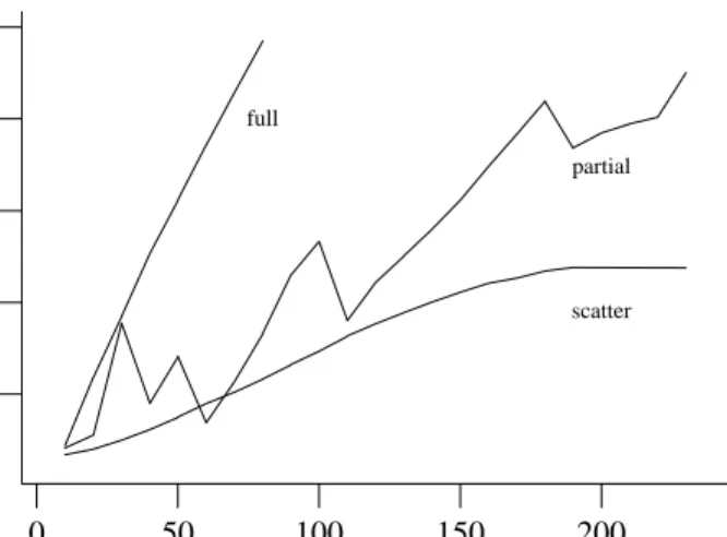
Figure 1 shows how the runtime of a validation varies with the search depth for these three different search modes. The queue size for the test protocol was fixed at two slots per queue in all measurements that fol-low, except those that specifically measured the effect of the queue size on validations.

0 50 100 150 200 10 100 1000 10000 100000 full partial scatter Seconds Search Depth Figure 1 − Runtime

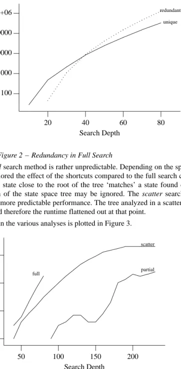
For the test protocol a full search became unfeasible beyond a search depth of 80 execution steps. To check just how much double work is caused by the overlaps in the full searches, Figure 2 compares the number of unique states to the total number of times that a previously analyzed state had to be analyzed again (dotted line). At a search depth of 80 steps the number of states searched is almost four times larger than would be required in a minimal search. For the test protocol this means that a search up to approximately 90 steps would be feasible if the redundancy of the overlaps could be avoided completely. The redundancy therefore has a noticeable effect, though not nearly as large as the effect of a change in the search discipline.

(3)

20 40 60 80 100 1000 10000 100000 1e+06 .... .... .. .... . . .. . . .. . .. .. . . .. . . ... . . .. . . ... . . .. .. .. . . .. . . . . unique redundant No. of States Analyzed Search Depth Figure 2 − Redundancy in Full Search

The complexity of the crude partial search method is rather unpredictable. Depending on the specific order in which the state space tree is explored the effect of the shortcuts compared to the full search can be more or less dramatic. If, for instance, a state close to the root of the tree ‘matches’ a state found close to the depth limit before, a large fraction of the state space tree may be ignored. The scatter search technique applied to a full search tree gives a more predictable performance. The tree analyzed in a scatter search had a maximum depth of 189 levels, and therefore the runtime flattened out at that point.

The number of deadlocks reported in the various analyses is plotted in Figure 3.

50 100 150 200 1 10 100 1000 scatter partial full Number of Deadlocks Search Depth Figure 3 − Deadlocks vs Search Depth

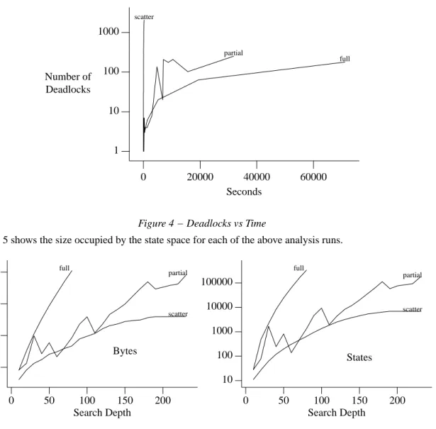
The number of deadlocks reported per test is not as such a reliable indication of the scope of the corre-sponding analysis method since one error can trigger a number of equivalent deadlock reports that varies with the search method used. Still, both the minimum search depth required for the first error report to appear and the relation between search depth and number of error reports generated are probably good indi-cations of the quality of the analysis. Under these two criteria, the scatter search method performs remark-ably well. Figure 4 plots the number of deadlocks reported versus the time it took to find them. Also these results are favorable for the scatter searching technique.

(4)

0 20000 40000 60000 1 10 100 1000 scatter partial full Number of Deadlocks Seconds Figure 4 − Deadlocks vs Time

Figure 5 shows the size occupied by the state space for each of the above analysis runs.

0 50 100 150 200 10000 100000 1e+06 1e+07 scatter partial full Bytes Search Depth 0 50 100 150 200 10 100 1000 10000 100000 scatter partial full States Search Depth Figure 5 − No. of Bytes and States in State Space Cache

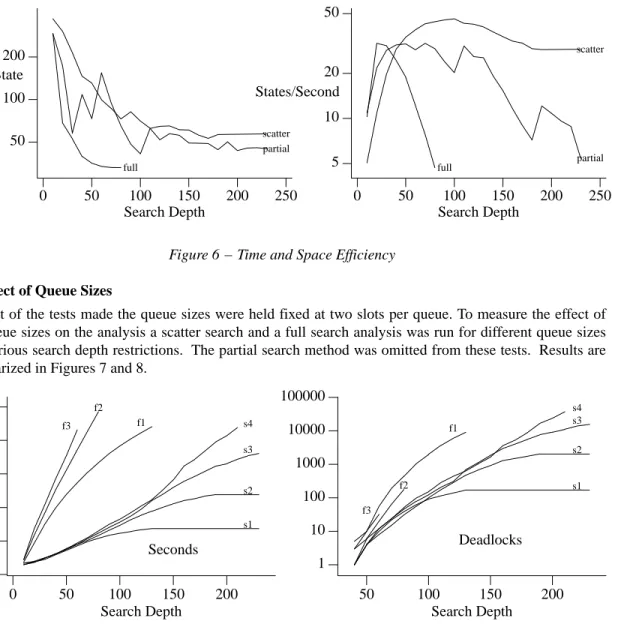
As can be expected, the rate at which the state space expands closely resembles the rate at which both the number of system states explored and the runtime (Figure 1) increases. In Figure 6, the average number of bytes used per state in the state space cache and the average number of states analyzed per second is plot-ted. The analyzer tries to exploit the use of state templates, lists of common subsets of information held in states, to minimize the total amount of storage used. Figure 6 illustrates that the effort pays off for the larger state spaces. It also shows that, beyond a certain limit the analysis will slow down as the state space grows. Since scatter searching generates a smaller state space this effect is not quite as large. For a large state space, however, scatter searching turns out to be the least space efficient method of the three strategies explored.

(5)

0 50 100 150 200 250 50 100 200 scatter partial full Search Depth Bytes/State 0 50 100 150 200 250 5 10 20 50 scatter partial full Search Depth States/Second

Figure 6 − Time and Space Efficiency 3. Effect of Queue Sizes

In most of the tests made the queue sizes were held fixed at two slots per queue. To measure the effect of the queue sizes on the analysis a scatter search and a full search analysis was run for different queue sizes and various search depth restrictions. The partial search method was omitted from these tests. Results are summarized in Figures 7 and 8.

0 50 100 150 200 1 10 100 1000 10000 100000 s1 s2 s3 s4 f1 f2 f3 Seconds Search Depth 50 100 150 200 1 10 100 1000 10000 100000 s1 s2 s3 s4 f1 f2 f3 Deadlocks Search Depth Figure 7 − Effect of Queue Sizes on Runtime and Deadlocks Found

s − scatter search; f − full search; 1,2,3,4 − queue sizes

The complete state space tree of the scatter search for a queue size of one slot per queue (s1) is only 130 levels deep. For two slots per queue (s2) the state space tree grows to 190 levels. For three slots per queue (s3) the the state space tree is larger than 230 levels, the maximum depth explored in these tests. A scatter search in a tree of 200 levels deep takes roughly ten times longer with the addition of each slot to the queues.

(6)

0 50 100 150 200 10000 100000 1e+06 1e+07 s1 s2 s3 s4 f1 f2 f3 Bytes Search Depth 0 50 100 150 200 10 100 1000 10000 100000 s1 s2 s3 s4 f1 f2 f3 States Search Depth Figure 8 − Effect of Queue Sizes on State Space

A full search (f1-3) invariably takes orders of magnitude more time to complete than a scatter search. Expanding the queue sizes enhances this effect, though not quite as dramatically as the step from a scatter search to a full search. Although it is rather difficult to compare the value to an actual user of an analysis that produces a listing of 15,645 deadlocks (s3 at maximum depth 230) to one that produces ‘only’ 32 (f3 at depth 60), it is likely that the former does indeed cover more cases.

The left hand side of Figure 9 shows the increase in runtimes when the search depth is fixed at 120, 140, 160 and 200 levels in the state space tree and the queue size is varied from 1 to 10 slots per queue. Clearly, the effect is more severe for larger state spaces.

100 1000 10000 120 200 160 140 1 2 3 4 5 6 7 8 9 10 Seconds Queue Size 120 200 160 140 1 2 3 4 5 6 7 8 9 10 5 10 20 50 States/Second Queue Size Figure 9 − Search Depth and Queue Sizes (scatter search)

On the right hand side in Figure 9 the number of states analyzed per second of runtime is shown. The queue size, can be seen to have a quite dramatic effect on the number of states analyzed per second, worse still if the size of the state space increases.

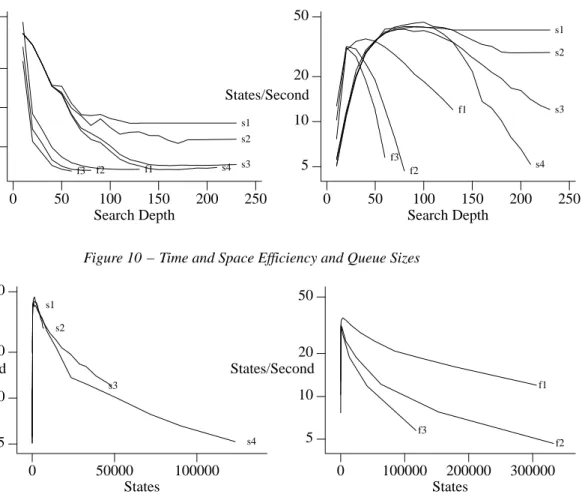
In Figure 10 the number of bytes used per state and the number of states analyzed per second is shown, for each combination of queue size and search depth. The results of Figures 6 and 9 are confirmed. The steep left ends of the curves can be attributed to the overhead involved in the setup of a state space, which is felt more if the number of states explored is small. The use of state templates results in a lower number of bytes per state as the queue size is expanded.

Figure 11 shows, separately for the scatter searches and the full searches, the number of states analyzed per second as a function of the total number of states in the state space. The figure shows that degradation of the performance is not solely caused by a growing state space: the queue sizes contribute to the complexity.

(7)

0 50 100 150 200 250 50 100 200 500 s1 s2 s3 s4 f1 f2 f3 Search Depth Bytes/State 0 50 100 150 200 250 5 10 20 50 s1 s2 s3 s4 f1 f2 f3 Search Depth States/Second

Figure 10 − Time and Space Efficiency and Queue Sizes

0 50000 100000 5 10 20 50 s1 s2 s3 s4 States States/Second 0 100000 200000 300000 f1 f2 f3 States States/Second 5 10 20 50

Figure 11 − Time Efficiency and State Space Size 4. Effect of Caching Discipline

For a protocol of realistic size and a search of sufficient depth there will be a point where the state space tree will no longer fit the amount of available memory. During the analysis the program trace holds (a selection of) previously visited states in a cache of fixed size to prune the state space tree wherever double work can be avoided. Initially, all system states encountered can simply be accommodated in the cache. When the cache fills up, though, a caching discipline is needed to decide which states can be deleted and which should be stored. Tw o factors will determine the efficiency of an analysis when state spaces larger than the cache are explored: the number of states that can be stored and the replacement strategy.

4.1. Replacement Strategies

Though the size of the cache can affect the runtime or even the feasibility of an analysis, it is irrelevant to its scope. Extending the size of the cache to the maximum that can fit in main memory can only avoid dou-ble work.

An important question is what the selection criterion should be for determining which states can be over-written when the cache fills up. One potentially relevant piece of information on the probability that a state will be revisited in a different part of the state space tree is the number of times that it was visited before.

(8)

0 10 20 30 40 10

100 1000 10000

Numbers of States Av erage Depth

Number of Visits

50

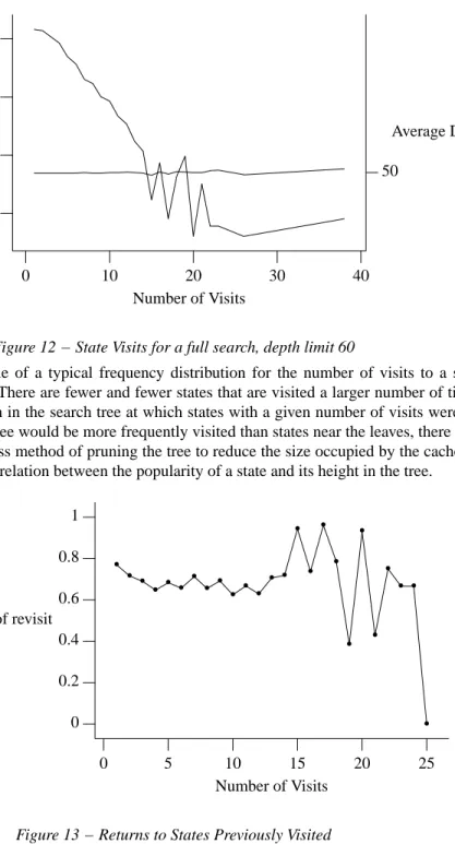
Figure 12 − State Visits for a full search, depth limit 60

Figure 12 gives an example of a typical frequency distribution for the number of visits to a state. Most states are only seen once. There are fewer and fewer states that are visited a larger number of times. Also plotted is the average depth in the search tree at which states with a given number of visits were found. If states near the root of the tree would be more frequently visited than states near the leaves, there would be a clean and relatively harmless method of pruning the tree to reduce the size occupied by the cache. Unfortu-nately, Figure 12 shows no relation between the popularity of a state and its height in the tree.

0 5 10 15 20 25 • • • • • • • • • _• • _• • • • • • • • • • • • • • Probability of revisit Number of Visits 0 0.2 0.4 0.6 0.8 1

Figure 13 − Returns to States Previously Visited

Figure 13 shows the probability of a return to a previously visited state given that a state was visited N times before. Up to 15 visits then, this probability is largely independently of the history of a state. Above that the behavior is somewhat erratic, until the probability drops to zero for the most frequently visited states. Clearly, members of this class of ‘most frequently visited states could safely be deleted from the cache, if only we could know a priori what the largest number of visits to a state was going to be.

For the test protocol the performance of four different cache replacement strategies was measured.

In the first strategy the states were divided dynamically in classes according to the number of times they had been visited before in the search. To replace a state the state space cache was scanned round-robin until a state was found that belonged to the currently

(9)

of states under this criterion. In the next strategy the number of previous visits to a state was ignored. The cache was viewed as a circular buffer. To replace a state with this strategy the one was selected that hap-pened to be pointed to by a round-robin pointer:

(b) blind, round-robin

selection. In the last two strategies the depth at which a state was last encountered in the tree was used as a selection criterion. States near the root of the tree are also roots of the largest subtrees. To replace a state, therefore, it should be advantageous to select a victim as deep in the tree as possible. In the third method therefore a lookup table of states was maintained organized in tree levels. States to be deleted were selected via the lookup table which guaranteed that at each point one of the currently

(c) lowest states

would be deleted. In the last replacement strategy tested a simpler list of only the (d) leaf states

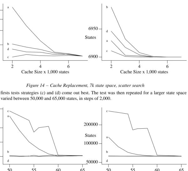
in the tree was maintained. Whenever a state had to be deleted the first state in that list was selected. If the list was empty a blind round-robin selection according to strategy (b) above was used. The behavior of the analyzer was first tested on a small cache of 6,900 states, reduced in steps of 1,000 states down to a cache size of only 2,000 states. The results are shown in Figure 14.

2 4 6 300 400 500 600 b a c d Seconds

Cache Size x 1,000 states

2 4 6 6900 6950 b a c d States

Cache Size x 1,000 states Figure 14 − Cache Replacement, 7k state space, scatter search

In these firsts tests strategies (c) and (d) come out best. The test was then repeated for a larger state space that was varied between 50,000 and 65,000 states, in steps of 2,000.

50 55 60 65 5000 10000 20000 50000 b a c d Seconds

50 55 60 65 50000 100000 200000 b a c d States

Cache Size x 1,000 states Figure 15 − Cache Replacement, 65k state space, full search, depth limit 60

In these tests strategy (d) proved superior to strategy (c). It is unclear why (d) is not consistently better than (c) or even why the difference between (c) and (d) is so large in the second series of tests. Quite

(10)

remarkably, in the larger state space the simple strategy (b) performs almost as well as the more subtle (d), while consuming less memory. In Figure 16 the curves for the best two strategies (b) and (d) are compared for further reductions than are feasible for (a) or (c).

30 40 50 60 6000 8000 10000 12000 db Seconds

30 40 50 60 100000 150000 200000 b d States

Cache Size x 1,000 states Figure 16 − Cache Replacement, 65k state space, full search, depth limit 60

Clearly, the effect of a better replacement strategy makes considerably larger state space reductions possi-ble. In this case, the state space cache could be reduced to less than 50% of the full cache size for a runtime penalty of only 20%. In this test, the two best strategies turn out to be almost indistinguishable with respect to runtime. Strategy (d), however, is slightly more selective in the generation of redundant deadlock reports (see appendix B).

The one strategy based on the previous number of visits to a state (a) (as well as two others described in [2]) does not perform well at all.

Cache replacement strategy (d) is the default in the analyzer. 4.2. Cache Sizes

Using replacement strategy (d) the effect of a series of reductions of a large state space cache was mea-sured. The results shown in Figure 17 are from full searches in a fixed size state space tree of 70 levels deep. The cache size was varied from a full cache of 150,000 states to a restricted cache of 45,000 states in steps of 1,000. 50 100 150 20000 50000 100000 Seconds

50 100 150

200000 500000 1e+06

States

Cache Size x 1,000 states Figure 17 − Cache Size, 150k state space, full search, depth limit 70

The restriction of the cache has little effect on the performance of the analyzer up to a certain limit beyond which analysis will quickly become unfeasible. As in the test of Figure 16 the limit was found at a reduc-tion to approximately 40-50% of the full cache size.

(11)

5. Conclusion

The test results documented in this report can provide some insight into the complexity of protocol analy-sis. We hav e shown that simple exhaustive analyses can hardly be expected to produce results of interest for protocols of the size tested here. We hav e also obtained some quantitative results on the substantial effect that increments in queue sizes and search depths can have on runtime and state space size for various search disciplines. The program trace is an effort to develop a tool that can be used to probe the state space of protocols that are normally beyond the scope of automated analyzers. The main tools for restricting a search in trace, then, are the queue size restrictions, search depth restrictions and the use of the scatter search discipline [2].

Tr ace maintains a cache of system states that, as need dictates, can be made either larger or smaller than the size of the state space to be searched. If the cache is smaller, a cache replacement strategy is used to decide which states are to be deleted from the cache when it is about to overflow. The effect of this cache replace-ment strategy was found to be decisive for the feasibility of analysis. Four different strategies were tested and quite remarkably we found that the least sophisticated methods were superior in almost every case of interest. With the best cache replacement strategy cache size restrictions of roughly 50% were shown to be feasible with only minor runtime penalties.

(12)

6. References

1. "Trace - a protocol analyzer", AT&T Bell Laboraties, internal report, May 22, 1984, 27 pgs.

2. "Automated protocol validation in Argos, assertion proving and scatter searching," AT&T Bell Labo-raties, internal report, August 8, 1984, 23 pgs.

(13)

7. Appendix A: The Test Protocol

A full listing in the validation language Argos [1,2] of the protocol used for the performance tests is given below. The protocol compiler pret translates this desciption into a lower level description consisting of 3 variables, 6 message queues and 4 finite state machines of respectively 31, 50, 7, and 5 states. The 4 pro-cesses exchange 32 different types of messages. One incompleteness error in the description as specified is flagged by the compiler, but ignored in the tests: the messages ‘adial,’ ‘nak,’ and ‘call’ are received but not sent. proc host { queue h_normal[10]; queue h_extern[10]; pvar n; closed: do :: h_normal?close −> c_normal!aclose :: h_normal?aclose −> skip :: h_normal?adial −> skip

:: h_normal?talk −> c_normal!close; goto lclosed

:: h_normal?atalk −> skip :: h_normal?nak(n) −> if :: (n == 0) −> goto fail :: (n != 0) −> c_normal!close fi

:: h_extern?opent −> c_normal!talk; goto watalk :: h_extern?opend −> c_normal!dial; goto wadial od;

dialing: do

:: h_normal?close −> c_normal!aclose; goto rclosed

:: h_normal?adial −> skip

:: h_normal?talk −> c_normal!atalk; h_envirn!htalk; goto talking

:: h_normal?atalk −> skip

:: h_extern?sysclose −> c_normal!close; goto lclosed od;

talking: do

:: h_normal?talk −> c_normal!atalk

:: h_extern?sysclose −> c_normal!close; goto lclosed

:: h_extern?ioattn −> c_normal!dial; goto wattn

od; rclosed:

do

:: h_normal?close −> c_normal!aclose

:: h_extern?sysclose −> c_normal!close; goto lclosed od;

watalk: do

(14)

:: h_normal?atalk −> goto wtalk :: h_normal?nak(n) −> if :: (n == 0) −> goto fail :: (n != 0) −> skip fi

:: h_extern?timeout −> c_normal!talk od; wadial: do :: h_normal?close −> c_normal!aclose :: h_normal?aclose −> skip

:: h_normal?adial −> goto dialing

:: h_normal?atalk −> skip :: h_normal?nak(n) −> if :: (n == 0) −> goto fail :: (n != 0) −> skip fi

:: h_extern?timeout −> c_normal!dial

od; lclosed:

do

:: h_normal?aclose −> goto closed

:: h_normal?talk −> c_normal!atalk; c_normal!close

:: h_normal?atalk −> skip :: h_normal?nak(n) −> skip :: h_extern?sysclose −> skip :: h_extern?timeout −> c_normal!close od; wtalk: do

:: h_normal?talk −> c_normal!atalk; goto talking

:: h_normal?nak(n) −> goto closed

:: h_extern?sysclose −> c_normal!close od;

wattn: do

:: h_normal?adial −> goto dialing

:: h_normal?talk −> c_normal!atalk

:: h_extern?sysclose −> c_normal!aclose; goto lclosed

:: h_extern?timeout −> c_normal!dial

od; fail:

do

(15)

:: h_extern?sysclose −> skip od } proc cont { queue c_normal[10]; queue c_extern[10]; pvar n; pvar pvc; idle: do :: c_normal?close −> h_normal!aclose :: c_normal?aclose −> skip

:: c_normal?dial −> h_normal!adial; c_envirn!trans; goto dialing

:: c_normal?adial −> skip :: c_normal?talk −> if :: (pvc == 0) −> goto wproc :: (pvc != 0) −> goto wcall fi :: c_normal?atalk −> skip :: c_normal?nak(n) −> if :: (n == 0) −> goto fail :: (n != 0) −> h_normal!close fi :: c_extern?call −> c_envirn!cnak od; dialing: do

:: c_normal?close −> h_normal!aclose; goto idle

:: c_normal?dial −> h_normal!adial

:: c_extern?call −> c_envirn!cnak

:: c_extern?cnak −> h_normal!nak(1); goto wclose

:: c_extern?transok −> c_envirn!call; goto wproc od;

talking: do

:: c_normal?close −> h_normal!aclose; c_envirn!hangup; goto idle

:: c_normal?dial −> h_normal!adial; goto dialing

:: c_normal?talk −> h_normal!atalk

:: c_normal?atalk −> skip

:: c_extern?hangup −> h_normal!close; goto lclosed od;

wcall: do

:: c_extern?call −> c_envirn!numb; goto wnumb

od; wnumb:

(16)

do

:: c_extern?numbis −> h_normal!talk; c_envirn!answer; goto watalk od;

watalk: do

:: c_normal?atalk −> goto talking

:: c_extern?hangup −> h_normal!close; goto lclosed :: c_extern?timeout −> h_normal!talk

od; wclose: do

:: c_normal?dial −> h_normal!adial :: c_normal?adial −> skip :: c_normal?talk −> h_normal!atalk :: c_normal?atalk −> skip :: c_extern?call −> c_envirn!cnak od; lclosed: do

:: c_normal?aclose −> goto idle

:: c_normal?dial −> h_normal!adial; h_normal!close

:: c_normal?adial −> skip

:: c_normal?talk −> h_normal!atalk; h_normal!close

:: c_normal?atalk −> skip :: c_normal?nak(n) −> if :: (n == 0) −> goto fail :: (n != 0) −> h_normal!close fi :: c_extern?call −> c_envirn!cnak :: c_extern?timeout −> h_normal!close od; wproc: do

:: c_extern?answer −> h_normal!talk; goto watalk

:: c_extern?numb −> c_envirn!numbis

od; fail:

(17)

:: c_normal?nak(n) −> skip :: c_extern?call −> c_envirn!cnak od } proc cenvir { queue c_envirn[10]; /* * c_extern!call; */ do :: c_envirn?numbis −> if :: c_extern!answer :: c_extern!hangup fi :: c_envirn?trans −> if :: c_extern!transok :: c_extern!cnak fi :: c_envirn?answer −> c_extern!hangup :: c_envirn?cnak −> skip :: c_envirn?hangup −> skip :: c_envirn?numb −> if :: c_extern!numbis :: c_extern!hangup fi :: c_envirn?call −> if :: c_extern!numb :: c_extern!cnak fi od } proc henvir { queue h_envirn[10]; idle: if

:: h_extern!opent; goto open :: h_extern!opend; goto open fi;

open: if

:: h_extern!sysclose; goto idle

(18)

fi; talking:

if

:: h_extern!sysclose

:: h_extern!ioattn; goto open fi

(19)

8. Appendix B: Data

The tables below giv e the data used to plot the graphs in the body of the paper. Depth gives the number of levels in the state space tree analyzed. Nodes are state templates used to minimize the amount of memory used to store a state. Returns counts the number of times that a previously visited state was encountered during an analysis. Zapped counts the number of states that were deleted from the state space cache. It is zero in most of the tests, except in those in which cache replacement strategies or the effect of restricted cache sizes were tested. Loops is the number of execution loops detected in the protocol tested. Locks is the number of deadlocks reported. Bytes measures the size of the state space cache. Edges counts the num-ber of edges traversed in the state space tree during an analysis run.

8.1. Figures 1, 3, 4, 5, and 6

Scatter Search

depth seconds nodes states returns zapped loops locks bytes edges

10 2.18 10 11 0 0 0 0 4096 16 20 2.50 18 27 1 0 1 0 8192 44 30 3.15 35 62 1 0 1 0 13312 102 40 4.12 49 119 7 0 4 1 17408 202 50 5.62 61 196 10 0 7 4 25600 333 60 7.90 75 308 19 0 10 8 30720 519 70 10.50 88 449 27 0 13 15 38912 761 80 14.62 97 646 38 0 19 31 47104 1099 90 20.92 113 950 49 0 22 56 77824 1588 100 29.28 130 1352 57 0 24 100 95232 2241 110 42.90 143 1849 69 0 29 176 115712 3029 120 58.67 162 2497 78 0 31 289 161792 4004 130 77.05 169 3143 82 0 32 474 204800 5014 140 100.50 173 3786 90 0 32 683 231424 6021 150 129.20 181 4538 93 0 34 919 276480 7201 160 161.67 181 5296 95 0 34 1294 296960 8353 170 183.28 181 5818 95 0 34 1506 309248 9135 180 219.97 181 6408 95 0 34 1742 362496 10057 190 239.77 181 6900 95 0 34 2048 391168 10731 230 239.05 181 6900 95 0 34 2048 395264 10731

(20)

Partial Search

10 2.57 20 28 3 0 0 0 8192 43 20 3.55 35 77 58 0 5 0 13312 107 30 59.27 313 1684 3591 0 14 0 97280 2889 40 7.92 72 245 309 0 14 0 26624 404 50 25.80 166 811 1609 0 22 0 59392 1373 60 4.85 40 139 121 0 28 0 21504 207 70 13.68 110 434 725 0 28 0 40960 731 80 45.30 243 1322 2996 0 28 0 86016 2256 90 197.15 520 4709 10395 0 42 1 228352 8086 100 463.00 593 9354 20077 0 79 3 387072 15879 110 63.62 334 1931 3185 0 92 4 120832 3400 120 165.65 534 4282 9505 0 75 7 222208 7776 130 319.37 792 8115 17436 0 125 7 465920 13755 140 623.40 663 11924 29694 0 127 4 666624 20812 150 1295.48 754 19849 46229 0 149 4 976896 34112 160 3032.83 1060 35082 83403 0 264 8 1722368 61119 170 6799.00 1390 60946 150594 0 328 20 2979840 109404 180 15628.05 1713 111957 271805 0 466 103 4938752 198915 190 4814.12 1332 58225 133247 0 432 136 2923520 102288 200 7034.52 1770 75979 180584 0 540 208 3315712 135872 210 8813.38 1461 84512 204791 0 479 176 3834880 150411 220 10423.12 1537 91958 215343 0 547 208 4194304 162712 230 31813.87 2241 172402 434648 0 792 252 7725056 313755 Full Search

10 2.73 20 28 3 0 0 0 8192 43 20 15.18 118 481 808 0 5 0 32768 788 30 70.57 336 2155 4347 0 16 0 113664 3697 40 343.22 597 8372 18728 0 20 3 331776 14168 50 1306.60 927 24499 58224 0 29 6 868352 42798 60 5181.37 1298 63051 155517 0 41 20 2118656 111249 70 19444.58 1769 151739 384394 0 48 64 5008384 270865 80 71073.11 2374 332527 869060 0 64 179 10953728 603102

(21)

8.2. Figure 2

Full Search

depth unique redundant

10 28 0 20 481 45 30 2155 1090 40 8372 8917 50 24499 40889 60 63051 148997 70 151739 457856 80 332527 1264470 8.3. Figures 7, 8, 10 and 11

Scatter Search, Queue Size: 1

10 1.95 10 11 0 0 0 0 4096 16 20 2.38 18 27 1 0 1 0 8192 44 30 2.83 35 62 1 0 1 0 13312 102 40 3.90 51 117 7 0 4 1 17408 199 50 5.23 72 182 10 0 7 4 26624 313 60 7.13 89 284 17 0 9 10 30720 483 70 9.65 112 393 25 0 11 22 34816 675 80 12.05 124 508 31 0 14 39 44032 861 90 14.83 138 635 36 0 15 63 56320 1074 100 17.12 144 732 38 0 15 92 60416 1229 110 19.17 149 812 38 0 15 115 64512 1355 120 21.53 154 902 38 0 15 140 68608 1505 130 23.37 155 955 38 0 15 171 72704 1582 230 23.37 155 955 38 0 15 171 72704 1582

(22)

10 2.18 10 11 0 0 0 0 4096 16 20 2.50 18 27 1 0 1 0 8192 44 30 3.15 35 62 1 0 1 0 13312 102 40 4.12 49 119 7 0 4 1 17408 202 50 5.62 61 196 10 0 7 4 25600 333 60 7.90 75 308 19 0 10 8 30720 519 70 10.50 88 449 27 0 13 15 38912 761 80 14.62 97 646 38 0 19 31 47104 1099 90 20.92 113 950 49 0 22 56 77824 1588 100 29.28 130 1352 57 0 24 100 95232 2241 110 42.90 143 1849 69 0 29 176 115712 3029 120 58.67 162 2497 78 0 31 289 161792 4004 130 77.05 169 3143 82 0 32 474 204800 5014 140 100.50 173 3786 90 0 32 683 231424 6021 150 129.20 181 4538 93 0 34 919 276480 7201 160 161.67 181 5296 95 0 34 1294 296960 8353 170 183.28 181 5818 95 0 34 1506 309248 9135 180 219.97 181 6408 95 0 34 1742 362496 10057 190 239.77 181 6900 95 0 34 2048 391168 10731 230 239.05 181 6900 95 0 34 2048 395264 10731

10 1.98 10 11 0 0 0 0 4096 16 20 2.30 18 27 1 0 1 0 8192 44 30 3.13 35 62 1 0 1 0 13312 102 40 4.10 49 119 7 0 4 1 17408 202 50 5.90 61 200 10 0 7 6 25600 337 60 8.00 70 332 19 0 10 12 29696 543 70 11.88 77 499 27 0 13 24 34816 835 80 17.22 88 741 42 0 23 46 47104 1220 90 25.63 95 1104 57 0 26 79 63488 1810 100 36.68 105 1569 69 0 32 124 79872 2561 110 54.57 110 2300 86 0 42 209 100352 3711 120 89.10 120 3436 97 0 44 311 137216 5567 130 160.30 134 5422 117 0 51 693 207872 8335 140 245.33 147 7492 131 0 57 1125 273408 11487 150 398.35 162 10656 141 0 62 1862 384000 15906 160 602.35 171 14465 159 0 67 2988 519168 21101 170 841.18 178 17951 171 0 71 4072 648192 26157 180 1200.37 186 23294 174 0 73 5662 840704 33579 190 1710.98 187 28630 188 0 77 7701 1033216 40774 200 2019.87 187 32606 188 0 77 9197 1176576 46318 210 2728.22 187 38378 188 0 77 11193 1389568 54198 220 3464.32 187 44422 188 0 77 14069 1618944 62366 230 4004.00 187 48162 188 0 77 15645 1762304 67434

(23)

10 2.17 10 11 0 0 0 0 4096 16 20 2.40 18 27 1 0 1 0 8192 44 30 3.07 35 62 1 0 1 0 13312 102 40 4.18 49 119 7 0 4 1 17408 202 50 5.82 61 202 10 0 7 4 25600 339 60 8.77 70 340 19 0 10 12 29696 551 70 12.70 75 525 27 0 13 24 34816 865 80 19.98 77 825 42 0 23 51 47104 1330 90 31.38 84 1254 65 0 34 99 67584 2012 100 44.70 92 1813 77 0 40 153 83968 2893 110 69.53 99 2699 110 0 58 287 108544 4296 120 110.93 109 4014 129 0 68 445 149504 6303 130 171.02 111 5791 149 0 75 637 206848 9179 140 327.92 116 8965 188 0 90 1036 305152 14082 150 662.72 126 14311 208 0 103 1658 477184 22110 160 1723.93 134 23532 227 0 108 3646 789504 34528 170 2714.60 157 33360 260 0 116 5376 1115136 48797 180 4953.25 174 50237 283 0 135 9032 1701888 70628 190 9152.80 196 71694 307 0 142 17006 2459648 99348 200 13793.53 208 90418 337 0 146 24115 3098624 126019 210 23831.82 216 123247 354 0 156 37349 4274176 170282

Full Search, Queue Size: 1

10 2.35 17 18 1 0 0 0 8192 29 20 8.75 100 263 335 0 5 0 23552 432 30 32.28 287 1108 1740 0 10 0 74752 1881 40 98.18 492 3504 6062 0 12 3 173056 5947 50 243.65 769 8365 14653 0 12 10 349184 14357 60 540.08 1034 16983 30396 0 19 56 642048 29464 70 1130.22 1373 31567 57094 0 42 193 1132544 55328 80 2152.70 1660 52723 96686 0 79 440 1827840 93755 90 4032.97 1960 84070 155747 0 101 1065 2860032 151407 100 6836.48 2201 126600 236700 0 122 2008 4268032 230174 110 11030.32 2393 178136 334823 0 162 3709 5976064 328465 120 16975.52 2606 238073 447680 0 221 6077 7983104 443540 130 25519.52 2793 306030 580905 0 292 9111 10273792 576527

10 2.73 20 28 3 0 0 0 8192 43 20 15.18 118 481 808 0 5 0 32768 788 30 70.57 336 2155 4347 0 16 0 113664 3697 40 343.22 597 8372 18728 0 20 3 331776 14168 50 1306.60 927 24499 58224 0 29 6 868352 42798 60 5181.37 1298 63051 155517 0 41 20 2118656 111249 70 19444.58 1769 151739 384394 0 48 64 5008384 270865

(24)

10 2.83 20 36 3 0 0 0 8192 51 20 23.77 118 744 1407 0 5 0 40960 1209 30 124.45 336 3383 7456 0 16 0 150528 5755 40 727.12 597 13686 32460 0 20 5 491520 23211 50 3493.28 927 41317 103725 0 30 10 1388544 71509 60 20440.35 1300 117808 313754 0 44 32 3843072 205336 8.4. Figure 9

Scatter Search, Depth 120

queue seconds nodes states returns zapped loops locks bytes edges

1 21.53 154 902 38 0 15 140 68608 1505 2 58.67 162 2497 78 0 31 289 161792 4004 3 89.10 120 3436 97 0 44 311 137216 5567 4 110.93 109 4014 129 0 68 445 149504 6303 5 167.15 95 4992 161 0 84 660 174080 7573 6 237.30 84 5928 193 0 116 818 198656 8765 7 337.75 79 7260 193 0 116 1178 240640 10121 8 453.15 79 8556 193 0 116 1630 282624 11553 9 668.43 79 10780 193 0 116 2414 349184 13841 10 1023.48 79 13420 193 0 116 3214 436224 16753

1 23.37 155 955 38 0 15 171 72704 1582 2 100.50 173 3786 90 0 32 683 231424 6021 3 245.33 147 7492 131 0 57 1125 273408 11487 4 327.92 116 8965 188 0 90 1036 305152 14082 5 462.38 110 10919 252 0 138 1686 354304 16272 6 784.20 99 13695 348 0 202 2392 428032 19896 7 1401.25 90 17891 412 0 266 3592 543744 24628 8 2285.03 79 22555 412 0 266 4804 680960 30100 9 3832.75 79 28747 412 0 266 6860 866304 36580 10 6495.95 79 36763 412 0 266 9484 1097728 45268

1 23.37 155 955 38 0 15 171 72704 1582 2 161.67 181 5296 95 0 34 1294 296960 8353 3 602.35 171 14465 159 0 67 2988 519168 21101 4 1723.93 134 23532 227 0 108 3646 789504 34528 5 1568.82 117 24809 339 0 172 3634 780288 37316 6 2350.85 111 29941 467 0 268 5369 915456 43532 7 5303.58 105 39569 659 0 396 8373 1183744 54524 8 10200.13 92 51785 787 0 524 12057 1530880 69044

(25)

1 23.37 155 955 38 0 15 171 72704 1582

2 239.77 181 6900 95 0 34 2048 391168 10731

3 2019.87 187 32606 188 0 77 9197 1176576 46318

4 13793.53 208 90418 337 0 146 24115 3098624 126019

8.5. Figures 12 and 13

Full Search, Depth 60 visits states average depth

1 14534 49 2 13798 49 3 10766 49 4 8452 49 5 4903 49 6 3635 49 7 2003 50 8 1712 49 9 1002 49 10 844 50 11 467 50 12 347 51 13 173 50 14 117 49 15 17 45 16 74 51 17 8 47 18 43 52 19 96 51 20 4 50 21 32 50 22 6 54 23 6 55 26 4 46 38 8 58

(26)

8.6. Figure 14

Scatter Search − 7k state space

size seconds nodes states returns zapped loops locks bytes edges noleaf

2/a 636.97 181 6929 98 4774 42 2052 223232 10782 0.0 2/b 304.82 181 6989 87 4834 56 2069 223232 10860 0.0 2/c 235.03 181 6911 91 4756 39 2055 223232 10746 0.0 2/d 275.23 181 6946 82 4791 49 2065 239616 10791 69.8 3/a 438.95 181 6903 96 3650 36 2048 301056 10736 0.0 3/b 286.50 181 6932 93 3679 49 2053 268288 10777 0.0 3/c 246.95 181 6901 94 3648 35 2049 268288 10732 0.0 3/d 260.20 181 6917 86 3664 40 2057 305152 10752 60.7 4/a 324.75 181 6902 96 2625 35 2048 346112 10733 0.0 4/b 273.53 181 6908 95 2631 41 2048 329728 10743 0.0 4/c 241.38 181 6900 95 2623 34 2048 333824 10731 0.0 4/d 258.82 181 6904 91 2627 36 2052 358400 10735 45.3 5/a 259.33 181 6900 95 1599 34 2048 366592 10731 0.0 5/b 254.63 181 6901 95 1600 37 2048 366592 10732 0.0 5/c 240.38 181 6900 95 1599 34 2048 366592 10731 0.0 5/d 247.47 181 6900 95 1599 35 2048 399360 10731 10.4 6/a 251.42 181 6900 95 575 34 2048 428032 10731 0.0 6/b 246.98 181 6900 95 575 36 2048 428032 10731 0.0 6/c 242.18 181 6900 95 575 34 2048 428032 10731 0.0 6/d 248.63 181 6900 95 575 34 2048 464896 10731 0.0 7/a 239.77 181 6900 95 0 34 2048 477184 10731 0.0 7/b 239.77 181 6900 95 0 34 2048 477184 10731 0.0 7/c 239.77 181 6900 95 0 34 2048 477184 10731 0.0 7/d 239.77 181 6900 95 0 34 2048 477184 10731 0.0

The first column in this and in the next three tables gives the cache sizes in multiples of 1,000 states. Where relevant the cache replacement strategy a, b, c, or d used is added as a suffix to the cache size. The last col-umn gives the percentage of cache replacements that could not be made with strategy (d) (see paper) because the list of ‘leaf’ states was depleted.

(27)

8.7. Figure 15

Full Search − 65k state space − Depth Limit 60

65/a 5181.37 1298 63051 155517 0 41 20 2118656 111249 0.0 60/a 5073.98 1298 63063 155539 325 41 20 2805760 111261 0.0 58/a 5662.48 1298 64117 159144 3427 41 20 2764800 113250 0.0 56/a 7181.42 1298 66775 168026 8133 41 20 2723840 117658 0.0 55/a 8523.68 1298 69106 173156 11488 41 20 2703360 121152 0.0 54/a 10125.00 1298 72439 182316 15845 41 20 2682880 126191 0.0 50/a 35348.28 1298 127143 334072 74645 41 20 2600960 218289 0.0 65/b 5181.37 1298 63051 155517 0 41 20 2118656 111249 0.0 60/b 5322.98 1298 63051 155517 313 41 20 2805760 111249 0.0 58/b 5259.45 1298 63051 155517 2361 41 20 2764800 111249 0.0 56/b 5087.75 1298 63061 155546 4419 41 20 2723840 111268 0.0 55/b 5280.52 1298 63072 155598 5454 41 20 2703360 111302 0.0 54/b 5068.93 1298 63091 155633 6497 41 20 2682880 111343 0.0 50/b 5236.63 1298 63527 157040 11029 41 23 1600960 112120 0.0 65/c 5181.37 1298 63051 155517 0 41 20 2118656 111249 0.0 60/c 5263.50 1298 65298 160188 2560 41 20 2805760 115164 0.0 58/c 21465.32 1298 176120 406037 115430 41 20 2764800 284905 0.0 56/c 20104.55 1298 174202 448742 115560 41 20 2723840 292557 0.0 55/c 16241.10 1298 165669 338500 108051 41 20 2703360 270010 0.0 54/c 28614.43 1298 298918 773116 242324 41 20 2682880 485026 0.0 50/c 45097.08 1298 333807 817328 281309 41 20 2600960 567058 0.1 65/d 5181.37 1298 63051 155517 0 41 20 2118656 111249 0.0 60/d 5066.20 1298 63051 155517 313 41 20 3059712 111249 0.0 58/d 5072.57 1298 63051 155517 2361 41 20 3014656 111249 0.0 56/d 5026.02 1298 63051 155517 4409 41 20 2969600 111249 0.0 55/d 5027.83 1298 63051 155517 5433 41 20 2945024 111249 0.0 54/d 5122.38 1298 63051 155517 6457 41 20 2924544 111249 0.0 52/d 4990.13 1298 63079 155509 8533 41 20 2875392 111283 0.0 50/d 5057.37 1298 63079 155509 10581 41 20 2822144 111283 0.0

(28)

8.8. Figure 16

Full Search − 65k state space − Depth Limit 60

65/b 5181.37 1298 63051 155517 0 41 20 2118656 111249 0.0 65/d 5181.37 1298 63051 155517 0 41 20 2118656 111249 0.0 60/b 5322.98 1298 63051 155517 313 41 20 2805760 111249 0.0 60/d 5066.20 1298 63051 155517 313 41 20 3059712 111249 0.0 58/b 5259.45 1298 63051 155517 2361 41 20 2764800 111249 0.0 58/d 5072.57 1298 63051 155517 2361 41 20 3014656 111249 0.0 56/b 5087.75 1298 63061 155546 4419 41 20 2723840 111268 0.0 56/d 5026.02 1298 63051 155517 4409 41 20 2969600 111249 0.0 55/b 5280.52 1298 63072 155598 5454 41 20 2703360 111302 0.0 55/d 5027.83 1298 63051 155517 5433 41 20 2945024 111249 0.0 54/b 5068.93 1298 63091 155633 6497 41 20 2682880 111343 0.0 54/d 5122.38 1298 63051 155517 6457 41 20 2924544 111249 0.0 52/b 5116.88 1298 63306 156040 8760 41 21 2641920 111741 0.0 52/d 4990.13 1298 63079 155509 8533 41 20 2875392 111283 0.0 50/b 5236.63 1298 63527 157040 11029 41 23 1600960 112120 0.0 50/d 5057.37 1298 63079 155509 10581 41 20 2822144 111283 0.0 48/d 5155.27 1298 63114 155519 12664 41 20 2781184 111342 0.0 48/b 5151.40 1298 63902 158533 13452 41 28 2564096 112903 0.0 46/d 5317.03 1298 63129 155515 14732 41 20 2736128 111365 0.0 46/b 5255.58 1298 64053 159230 15656 41 28 2523136 113230 0.0 44/d 5120.33 1298 63921 155289 17592 41 20 2482176 112389 9.0 44/b 5369.30 1298 64575 161380 18246 41 29 2281472 114114 0.0 42/d 5481.22 1298 67093 154712 22812 41 20 2269184 116263 15.9 42/b 5202.35 1298 65364 163691 21083 41 31 2240512 115534 0.0 40/d 5443.92 1298 70592 154079 28361 41 22 2215936 120660 20.5 40/b 5348.97 1298 66154 166772 23923 41 33 2199552 116942 0.0 38/d 5732.05 1298 73720 153809 33537 41 26 1904640 124637 24.2 38/b 5423.27 1298 68126 173840 27943 41 31 2154496 120843 0.0 36/d 5726.82 1298 77019 154386 38892 41 29 1859584 128839 27.1 36/b 5724.00 1298 71438 186549 33311 41 32 1847296 126929 0.0 34/d 5960.40 1298 79613 156643 43534 41 30 1810432 132341 30.3 34/b 6264.07 1298 78800 210762 42721 44 42 1773568 139511 0.0 32/d 6244.13 1298 92194 156205 58185 41 44 1728512 147724 27.3 32/b 6473.85 1298 82725 223801 48716 46 46 1732608 146367 0.0 30/d 6669.62 1298 105161 161137 73200 41 52 1683456 165779 26.8 30/b 7523.05 1298 94832 261324 62871 80 56 1527808 168620 0.0 28/d 7928.97 1298 124138 174149 94247 41 56 1634304 192047 26.7 28/b 8103.65 1298 102803 287956 72912 83 55 1486848 183091 0.0 26/d 9130.97 1298 147030 187362 119235 42 69 1585152 222154 26.3 26/b 12941.87 1298 161895 477192 134100 105 84 1445888 290018 0.0 24/d 11664.42 1298 201027 221368 175359 82 87 1531904 295791 24.8

(29)

8.9. Figure 17

Full Search, Depth 70

150 19444.58 1769 151739 384394 0 48 64 5008384 270865 0.0 145 20699.45 1769 151739 384394 1490 48 64 6699008 270865 0.0 135 19936.80 1769 151739 384394 11730 48 64 6150144 270865 0.0 125 19683.10 1769 151796 384378 22031 48 64 5912576 270948 0.0 115 18962.57 1769 151839 384359 32318 48 64 5404672 270992 0.0 105 19660.72 1769 159304 382436 50023 48 64 5158912 280163 18.2 95 20061.35 1769 175000 379452 75979 48 66 4663296 298406 25.8 85 22424.88 1769 200051 377164 111294 54 106 4429824 329100 27.8 75 23377.33 1769 244843 396476 166434 60 266 3917824 388995 28.7 65 29033.48 1769 307444 455467 239428 80 264 3667968 474246 31.4 55 39390.25 1769 476543 563933 418935 101 673 3028992 702352 28.5 45 94457.23 1769 1263740 1295694 1216456 519 1990 2582528 1814740 27.7