biophysically detailed neuronal network
modelling
Patrick John Gleeson
Department of Neuroscience, Physiology and Pharmacology
UCL
February 2012
This is a thesis submitted to the University of London in the Faculty of Life Sciences for the degree of Doctor of Philosophy. I confirm that the work presented is my own. Where information has been derived from other sources it has been indicated.
Increasingly detailed data are being gathered on the molecular, electrical and anatomical properties of neuronal systems both in vitro and in vivo. These range from the kinetic properties and distribution of ion channels, synaptic plasticity mechanisms, electrical activity in neurons, and detailed anatomical connectivity within neuronal microcircuits from connectomics data. Publications describing these experimental results often set them in the context of higher level network behaviour. Biophysically detailed com-putational modelling provides a framework for consolidating these data, for quantifying the assumptions about underlying biological mechanisms, and for ensuring consistency in the explanation of the phenomena across scales. Such multiscale biophysically detailed models are not currently in wide-spread use by the experimental neuroscience community however. Reasons for this include the relative inaccessibility of software for creating these models, the range of specialised scripting languages used by the available simulators, and the difficulty in creating and managing large scale network simulations.
This thesis describes new solutions to facilitate the creation, simulation, analysis and reuse of biophysically detailed neuronal models. The graphi-cal application neuroConstruct allows detailed cell and network models to be built in 3D, and run on multiple simulation platforms without detailed programming knowledge. NeuroML is a simulator independent language for describing models containing detailed neuronal morphologies, ion channels, synapses, and 3D network connectivity. New solutions have also been devel-oped for creating and analysing network models at much closer to biological scale on high performance computing platforms. A number of detailed
neo-with these tools.
The tools and models I have developed have already started to be used for original scientific research. It is hoped that this work will lead to a more solid foundation for creating, validating, simulating and sharing ever more realistic models of neurons and networks.
Abstract 2 List of Figures 9 List of Tables 12 List of Publications 13 Acknowledgements 15 1 Introduction 16
1.1 Computational modelling in scientific research . . . 16
1.2 Biophysically detailed neuronal modelling . . . 18
1.2.1 Classifying different approaches to neuronal modelling 19 1.2.2 Why model with high anatomical and biophysical detail? 23 1.2.3 Modelling active conductances . . . 27
1.2.4 Cable theory and compartmental modelling . . . 30
1.3 Current practices in detailed neuronal modelling . . . 33
1.3.1 Neuronal simulators . . . 34
1.3.2 Model publication, dissemination and reproducibility . 36 1.3.3 Accessibility and model reuse issues . . . 38
1.3.4 Biological variability versus mean model development 39 1.3.5 Generation and control of large scale network simula-tions . . . 40
1.3.6 Testing and validation of distributed model components 41 1.3.7 Comparison with Systems Biology field . . . 42
2.1.1 Motivation for developing neuroConstruct . . . 48
2.1.2 Implementation aspects . . . 51
2.1.3 Project structure . . . 53
2.2 Key features of neuroConstruct . . . 53
2.2.1 Neuronal morphologies in neuroConstruct . . . 55
2.2.2 Creation of conductance based cell models . . . 60
2.2.3 Network generation and visualisation . . . 66
2.2.4 Simulation management . . . 73
2.2.5 Network activity analysis . . . 73
2.2.6 Advanced features . . . 74
2.3 Interaction with other software packages . . . 75
2.3.1 Simulator support . . . 75
2.3.2 Other tools and languages . . . 78
2.4 Using neuroConstruct . . . 79
2.4.1 Installing and running neuroConstruct . . . 79
2.4.2 Documentation . . . 80
2.5 Conclusions . . . 80
3 NeuroML 82 3.1 The need for standardisation in computational neuroscience 82 3.2 The development of NeuroML . . . 83
3.2.1 Pre 2004 . . . 83
3.2.2 NeuroML version 1.x . . . 84
3.3 Structure of NeuroML version 1.x . . . 86
3.3.1 Technical approach to language specification . . . 86
3.3.2 Levels in NeuroML version 1.x . . . 88
3.3.3 Schemas for Levels . . . 98
3.4 Organisational structure of NeuroML . . . 99
3.5 Tool support for NeuroML . . . 101
3.5.1 NeuroML language specifications . . . 101
3.5.2 NeuroML Validator website . . . 102
3.5.3 NeuroML example models . . . 103
3.5.4 neuroConstruct . . . 104
3.5.8 PyNN . . . 112 3.5.9 NeuroMorpho.org . . . 113 3.5.10 TREES Toolbox . . . 114 3.5.11 CX3D . . . 114 3.5.12 NETMORPH . . . 115 3.6 NeuroML version 2.0 . . . 116 3.6.1 Limitations of NeuroML v1.x . . . 116
3.6.2 New features of NeuroML v2.0 . . . 117
3.6.3 Components and ComponentClasses . . . 118
3.6.4 libNeuroML . . . 121
3.7 Conclusions . . . 123
4 Simulation Management for Large Scale Network Models 124 4.1 Issues related to large scale network simulation . . . 125
4.1.1 Simulations on multiple processors . . . 127
4.1.2 Large data set management . . . 130
4.1.3 Limitations of GUI based approach . . . 131
4.1.4 Multiscale modelling . . . 132
4.2 Support for parallel network simulations in neuroConstruct . 133 4.2.1 Parallel NEURON . . . 133
4.2.2 Generic parallel simulation handling in neuroConstruct 135 4.2.3 Parallel NEURON generation from neuroConstruct . . 137
4.2.4 Interaction with remote computing hardware . . . 137
4.2.5 Performance measures . . . 138
4.2.6 Limitations . . . 144
4.3 Dealing with the data deluge: compact data representations 144 4.3.1 Network representations . . . 145
4.3.2 Simulation data sets . . . 147
4.4 Development of a Python based scripting interface . . . 149
4.4.1 Python in computational neuroscience . . . 149
4.4.2 Implementation in neuroConstruct using Jython . . . 150
4.5 Automated testing infrastructure . . . 154
4.6 Interacting with subcellular signalling pathways . . . 156
5.1.1 Cerebellar anatomy and physiology . . . 163
5.1.2 Theoretical and computational models of cerebellar function . . . 166
5.1.3 Cerebellar cell models . . . 168
5.1.4 Cerebellar network models . . . 174
5.2 Neocortical model development . . . 182
5.2.1 Anatomical and functional connectivity of the neocortex182 5.2.2 Neocortical modelling . . . 184
5.2.3 Neocortical and thalamic cell models . . . 185
5.2.4 Thalamocortical network models . . . 194
5.3 Models from other brain regions . . . 199
5.3.1 CA1 pyramidal cell model . . . 199
5.3.2 Dentate Gyrus network model . . . 201
5.4 Conclusions . . . 203
6 Validation and Evaluation 205 6.1 Validation criteria . . . 205
6.2 Evaluation . . . 207
6.2.1 Fulfilment of objectives . . . 207
6.2.2 Conclusions . . . 216
7 Discussion 218 7.1 Facilitating creation and analysis of 3D network models . . . 218
7.1.1 Enabling more realistic network models in 3D . . . 219
7.1.2 Accessibility of models . . . 222
7.1.3 Sharing model components . . . 223
7.1.4 Technology integration . . . 223
7.1.5 Usage of neuroConstruct . . . 224
7.2 Current state of standardisation and interoperability initiatives227 7.2.1 Evolution of the NeuroML initiative . . . 227
7.2.2 Improving model quality through cross simulator val-idation . . . 231
7.2.3 Community engagement . . . 232
7.3 Collaborative large scale model development . . . 234
1.1 Three possible ways to categorise neuronal modelling . . . 20
1.2 Diversity of neuronal morphologies and distribution of chan-nel densities . . . 26
1.3 A section of a dendrite illustrating the flow of electrical current 31 1.4 Modelling of dendrites as electrically connected compartments 32 2.1 The main neuroConstruct graphical user interface. . . 52
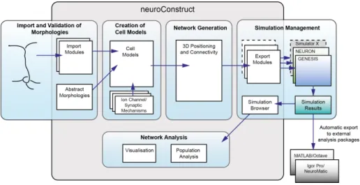
2.2 An overview of the core neuroConstruct functionality. . . 54
2.3 Various formats for representing neuronal morphologies . . . 59
2.4 Detailed cell morphologies in neuroConstruct. . . 61
2.5 Example of validating and transforming a NeuroML file . . . 64
2.6 Network connection types in neuroConstruct . . . 69
3.1 Example NeuroML file containing cells, channels, synapses and network elements . . . 87
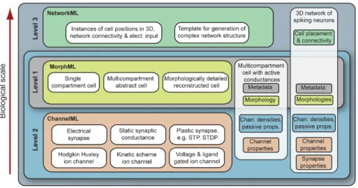
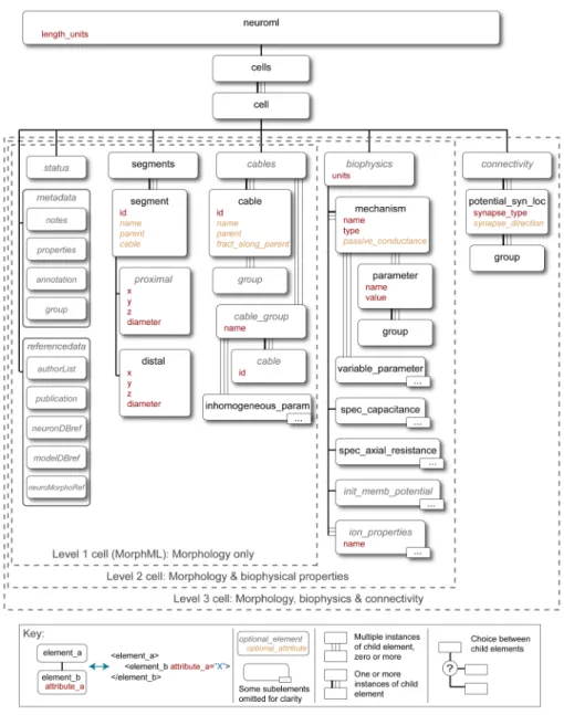
3.2 The three Levels in NeuroML version 1.x . . . 88
3.3 Elements for representing cells in NeuroML Levels 1-3. . . 91
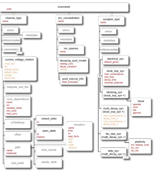
3.4 Elements in ChannelML. . . 92
3.5 Example of ChannelML file and mapping to text format and graphs . . . 94
application. . . 99 3.8 Online NeuroML Validator application . . . 102 3.9 Examples of models which are available in NeuroML . . . 104 3.10 A pyramidal cell visualised in neuroConstruct from a
Mor-phML cell description. . . 105 3.11 A pyramidal cell visualised in NEURON from a MorphML
cell description. . . 109 3.12 A pyramidal cell visualised in PSICS from a MorphML cell
description. . . 111 3.13 NeuroML file generated by the TREES Toolbox and loaded
into neuroConstruct . . . 115 3.14 NetworkML file generated by CX3D and loaded into
neuro-Construct . . . 116 3.15 Hierarchical structure of NeuroML v2.0 . . . 119 3.16 FitzHugh-Nagumo model cell specified in NeuroML v2.0 . . . 120 3.17 Import and export formats in libNeuroML . . . 122
4.1 Generation of parallel simulation code in neuroConstruct . . 136 4.2 Execution of parallel simulation code on remote compute nodes139 4.3 Parallel simulation of cerebellar granule cell layer . . . 142 4.4 Parallel simulation of cortical column . . . 143 4.5 NetworkML stored in HDF5 format . . . 146 4.6 Comparison of file sizes for NetworkML in different formats . 147 4.7 Example of Python script for controlling a neuroConstruct
simulation . . . 152 4.8 Hierarchy of tests which can be performed on neuroConstruct
5.1 Diagram of olivo-cerebellar system showing main cell types . 164
5.2 Cerebellar granule cell models . . . 170
5.3 Golgi cell models . . . 173
5.4 De Schutter and Bower (1994) Purkinje cell model . . . 175
5.5 Maex and Schutter (1998) granule cell layer model . . . 177
5.6 Pair of electrically connected Golgi cells from Vervaeke et al (2010) . . . 179
5.7 Vervaeke et al (2010) Golgi cell network model . . . 180
5.8 Initial version of 3D model of cerebellar cortex . . . 182
5.9 Mainen et al (1995) layer 5 pyramidal cell model . . . 186
5.10 Multiplicative gain modulation in a layer 5 pyramidal cell model188 5.11 Traub et al (2005) cell models . . . 191
5.12 Convergence of model behaviour for fine spatial discretisation 193 5.13 Cunningham et al (2004) L2/3 network model . . . 195
5.14 Connectivity matrix for Traub et al (2005) model . . . 196
5.15 Traub et al (2005) thalamocortical network model extended to 3D . . . 198
5.16 CA1 pyramidal cell model with non-uniform active conduc-tances . . . 200
5.17 Dentate gyrus model of Santhakumar et al (2005) . . . 202
7.1 Software applications which can interact with neuroConstruct and NeuroML . . . 225
7.2 Usage statistics for neuroConstruct . . . 226
2.1 Systems of units used in neuroConstruct, NEURON and
GEN-ESIS . . . 65
3.1 Features of NeuroML supported by simulators. . . 105
4.1 UCL based computing resources . . . 140
4.2 Simulation data set sizes . . . 148
5.1 Cell and network models converted to neuroConstruct/NeuroML format . . . 162
5.2 List of cell types used in Traub et al (2005) model . . . 189 5.3 List of active conductances used in Traub et al (2005) model 192
Journal Publications
Crook S, Gleeson P, Howell F, Svitak J, Silver RA (2007) MorphML: Level 1 of the NeuroML standards for neuronal morphology data and model specification. Neuroinformatics 5(2):96104
Cannon R, Gewaltig MO, Gleeson P, Bhalla U, Cornelis H, Hines M, Howell F, Muller E, Stiles J, Wils S, De Schutter E (2007) Interoperability of neuroscience modeling software: Current status and future directions. Neuroinformatics 5(2):127-138
Gleeson P, Steuber V, Silver RA (2007) neuroConstruct: a tool for mod-eling networks of neurons in 3D space. Neuron 54(2):219-235
Gleeson P, Crook S, Cannon RC, Hines ML, Billings GO, Farinella M, Morse TM, Davison AP, Ray S, Bhalla US, Barnes SR, Dimitrova YD, Sil-ver RA (2010) NeuroML: A language for describing data driven models of neurons and networks with a high degree of biological detail. PLoS Compu-tational Biology 6(6):e1000, 815
Vervaeke K, L˝orincz A, Gleeson P, Farinella M, Nusser Z, Silver RA (2010) Rapid desynchronization of an electrically coupled interneuron network with sparse excitatory synaptic input. Neuron 67(3):435451
Gleeson P, Silver RA, Steuber V (2010) Computer Simulation Environ-ments. In: Cutsuridis V, Graham B, Cobb S, Vida I (eds) Hippocampal Microcircuits: A Computational Modeler’s Resource Book, Springer Series in Computational Neuroscience, vol 5, Springer New York, pp 593-609
Gleeson P, Steuber V, Silver RA (2008) Using neuroConstruct to de-velop and modify biologically detailed 3D neuronal network models in health and disease. In: Soltesz I, Staley K (eds) Computational Neuroscience in Epilepsy, Academic Press, San Diego, pp 48-70
Gleeson P, Steuber V, Silver RA, Crook S (in press) NeuroML. In: Le Nov`ere N, Bhalla US (eds)Computational Systems Neurobiology, Springer
I would like to thank my supervisor Professor Angus Silver for guiding me through this process and for teaching me the importance of communicating ideas clearly. His emphasis on making the computational resources I have developed relevant for and accessible to the wider neuroscience community has been crucial in their successful uptake.
I am also very grateful to the current and past members Silver Lab. It has been an excellent environment for developing the tools and models described in this thesis, providing critical feedback from experimental, theoretical and computational points of view.
I would also like to thank the users of neuroConstruct and the wider Neu-roML community, especially Sharon Crook and Robert Cannon, for valuable contributions and feedback.
I thank my parents and family for all of their encouragement over the past number of years. Finally, I would like to thank my wife Anissa for her love and support during the long process of writing this thesis.
This work was supported by an MRC Special Research Training Fellow-ship in Bioinformatics and a Wellcome Trust Biomedical Resources Grant.
Introduction
1.1
Computational modelling in scientific research
The use of mathematical models in the physical sciences has a long history. Consolidating knowledge of a physical system into a set of equations which can be used to make predictions about its behaviour under specific condi-tions is one of the core activities in science. Physics has been particularly successful at creating succinct mathematical descriptions of natural phenom-ena which provide insight into the underlying principles of the world around us. When a system can be described by a small number of interacting enti-ties and a model created with a handful of variables, it is often possible to arrive at an analytical solution for the behaviour of the model (e.g. position in time of a planet moving around the sun or the rate of radioactive decay of atomic nuclei).
In many cases however, the complexity of the system under study does not allow a simple solution for how the state of the system will change with time, or behave under certain perturbations. While each element of the system may obey simple physical laws, how these interact to produce large scale system behaviour is not immediately obvious due to the nonlinear in-teraction of these elements (Gell-Mann, 1995). In recent years however, the use of computational modelling has greatly facilitated investigation of
the behaviour of such systems. Software representations of the equations describing the model can be created and multiple simulations run under dif-ferent input conditions or with difdif-ferent stochastic behaviour. Many fields have benefited from these advances (e.g. climate science, astrophysics, par-ticle physics, structural chemistry, epidemiology) and they have enabled researchers to make predictions about the activity of the physical systems under different conditions and gain insight into their underlying organisa-tional principles.
Computational modelling has become a core activity in physics, engineer-ing and chemistry and biologists are also startengineer-ing to benefit from encodengineer-ing knowledge of a biological system in a form amenable to use in simulations. The data deluge associated with genomics and DNA sequencing has led to a range of new computational techniques being used in the field, under the um-brella of bioinformatics. New researchers with computational backgrounds have entered biology and nowadays most biologists routinely use software packages to acquire, manage and analyse their data.
A large part of the computational modelling in biology (above the scale of structural molecular biology) is related to encoding knowledge about bio-chemical signalling pathways, which has led to the emergence of the field of Systems Biology (Kitano, 2002). There is also increasing work at the level of cellular interactions and indeed whole tissue modelling (Noble, 2002).
Neuroscientists too are increasingly encoding what is known about the anatomy and physiology of the nervous system at different biological scales in computer models. Use of these models by experimental neurobiologists has been slow however, despite over a hundred years of constructing mathe-matical models of neurons and networks (e.g. Lapicque’s 1907 work leading to the Integrate and Fire model (Brunel and van Rossum, 2007),
McCulloch-Pitts artificial neural networks (McCulloch and McCulloch-Pitts, 1943), Hodgkin Hux-ley squid axon model (Hodgkin and HuxHux-ley, 1952), Rall’s work on cable theory (Rall, 1959)). The work in this area has much to gain from expe-riences in other fields, not only technically (e.g. simulation algorithms, use of high performance computing), but also from the social point of view: how models and software are shared, how standards are developed and how modelling results are communicated to experimentalists in the field.
1.2
Biophysically detailed neuronal modelling
Neuroscience has a number of characteristics which distinguish it from many other areas of investigation in the physical sciences and make computa-tional modelling a vital tool for a greater understanding of the systems involved. Firstly, the elements which are involved are fundamentally multi-scale: explaining the behaviour of a microcircuit, neuron, active membrane or synapse will inevitably involve assumptions about the behaviour of an entity on a lower biological scale. Secondly, signalling and computation are distributed in space and time, and it is not usually apparent whether sub-cellular signalling, synaptic strengths, individual cell or population activity (or a combination of these) is the fundamental substrate of an information processing task. Thirdly, many neural systems consist of numerous repeated instances of subelements (channels, neurons, columns, etc). Computer mod-els are able to encode these hierarchical descriptions and easily make multi-ple repeated instances of subelements, in order to simulate the behaviour of the larger system under varying conditions. Finally, and most importantly, the elements of the nervous system interact in nonlinear ways, with different nonlinearities introduced at each biological scale. It is difficult to predict the effect pharmacological perturbations in the transition rates of a multi state
ion channel will have on the firing rate of a cell with the channel. A change in the release properties of synaptic vesicles can have multiple non-intuitive effects on the responsiveness of the postsynaptic cell. Clustering of different types of conductances on different regions of a dendritic tree can allow a cell to perform complex nonlinear computations on spatially segregated in-puts. These effects highlight the range of electrical, molecular and physical processes through which information is transformed in the nervous system, and the difficulties of inferring from a change in one level of the system the effect on the next. Well structured, data driven computer models encoding our assumptions of the behaviour of the different elements of the system are valuable tools towards gaining an insight into these complex multiscale interactions.
Before going onto more detail on the creation and analysis of multiscale models of neuronal systems and the software infrastructure available to sup-port them, it is useful to try to classify the wide range of approaches used in neuronal modelling.
1.2.1 Classifying different approaches to neuronal modelling
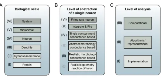
There are many endeavours which can be termed neuronal modelling (Dayan, 2006), each focussing on different biological scales of the nervous system, us-ing diverse assumptions on the core model elements, and various approaches to the analysis of the system behaviour (e.g. connectionist models of cog-nitive processing, firing rate models of connected brain areas, multicom-partmental conductance based models)1. To help classify these activities, a number of levels or scales have been devised to distinguish the approaches. These are summarised in Figure 1.1.
1
And consequently many different strands of research which are called Computational Neuroscience
Figure 1.1: Three possible ways which can be used to categorise neuronal modelling. A) The biological scale of elements included in the model, ranging from interactions at the protein level to systems level behaviour. B) The level of abstraction of the individual neuronal elements used, depending on how much of the physical, electrical and chemical properties of the cell are incorporated into the model. C) The level at which the function of the system is being analysed, whether it is the high level computation that the system is performing, the algorithm that is being used to process information and the way data is represented, or the specific implementation of the system in neuronal “hardware”.
A: Biological scales
A key way to classify neuronal models is by the biological scale of the el-ements included in the model (Figure 1.1A; Shepherd (2004)). Neuronal systems process information at multiple physical scales and can involve gene regulation mechanisms and protein signalling pathways (I), conduc-tance changes at synapses and distributed across membranes (II), compu-tations within dendritic subbranches (III) or across the neuron as a whole (IV).
Network processing can be carried out by local microcircuits (V), consist-ing of a small number of identified cell types carryconsist-ing out a specific function, or at a systems level (VI), where whole brain regions may be used as the
basic interacting units. Models of neuronal systems usually concentrate on one or a small number of these levels, and make approximations about the behaviour of the system at other levels. Multiscale neuronal models can be defined as models which incorporate biological detail at two or more of these levels.
B: Level of abstraction of individual neurons
Many neuronal models contain representations of individually active cells, and the level of abstraction of these towards or away from a complete bio-physical and electrical representation of the cell is another way to categorise such models (Figure 1.1B; Gerstner and Kistler, 2002; Herz et al, 2006). The highest level of biophysical detail (I) involves models incorporating the full 3D structure of the neurons, the electrical field potential inside the mem-brane, the diffusion and reaction of ions and molecules within this volume, and potentially the explicit location of membrane proteins (Blackwell, 2006; Coggan et al, 2005). Due to the high computational demands of such mod-els, it is more usual that only small sections of cells, e.g. spine heads, are modelled at this level of detail. Conductance based compartmental mod-els are more commonly used to simulate the electrical behaviour of cells in response to ion channels and synaptic input across the cell membrane. These can range in detail from cells based on morphological reconstruc-tions (II), abstract multicompartmental cells (III, with a reduced number of compartments used to investigate electrical behaviour in neurites) to single compartment cell models (IV, where the neuron is assumed to be electrically compact).
Integrate and Fire neurons (V) are a broad class of abstract neuron models which normally have just one or two state variables representing the
behaviour of the cells (i.e. membrane potential and potentially an adaptation or recovery variable). Realistic features of neurons including spiking, leaky integration of synaptic input and refractory periods are used to create an approximation of the electrical behaviour of cells, and more complex models have a small number of parameters which when set appropriately lead to voltage responses which mimic various classes of real neurons (Brette and Gerstner, 2005; Izhikevich, 2003)2. Cells can be represented as having con-tinuous valued firing rates (VI), and networks constructed where interactions depend on these rates and varying synaptic weights between cells.
The correct choice of level of abstraction of the neuronal elements in a model will be important and will crucially depend on the type and quality of experimental data available related to the phenomena being investigated.
C: Levels of analysis of neuronal models
A third way of distinguishing between models of what the nervous system is doing is based on the work of David Marr (Marr, 1982; Marr and Poggio, 1977). This approach developed from his work on understanding the visual system and describes some complementary levels of analysis for understand-ing how information is processed in neuronal systems (Figure 1.1C). The highest level (Computational) is that describing the general computation being performed (What is being computed? Why is this being done?). The second level (Algorithmic/representational) addresses how the computation is carried out, seeking a description of the algorithm used and how the re-quired data is represented and manipulated. The final level deals with the specific implementation of the operation in terms of neuronal structures.
2This level of abstraction of neuronal model should also include the classic
simpli-fications of the Hodgkin Huxley model such as the FitzHugh-Nagumo reduced model (FitzHugh, 1961) and the Morris-Lecar model (Morris and Lecar, 1981).
These three distinct ways of classifying neuronal modelling approaches will be useful in specifying the types of modelling addressed in this thesis, and will be referred back to later. While a subset of each scale has been focussed on in this work, it goes without saying that mathematical and computational models at all levels are valuable tools towards a greater understanding of brain function.
1.2.2 Why model with high anatomical and biophysical de-tail?
The tools and modelling languages which are the subject of this thesis facil-itate creating and analysing models at level I shown in Figure 1.1C. Models developed at this level are ideally accompanied by a clear description of the computational task being carried out by the system (level III) and the high level algorithm and data transformations being employed (level II). An iter-ative process of refinement of the description of the system at each of these levels of analysis is a feature of the development process of a good model (Gurney and Humphries, in press). One key question to ask then is what level of detail is most appropriate for the description of the “hardware” im-plementation of the model. Given that there are multiple types of neuronal models with varying degrees of complexity (Figure 1.1B), why not try to explain the behaviour of the system with the simplest base units possible? If simplified neuron models can be tuned to replicate the firing behaviour of a host of different cell types (Brette and Gerstner, 2005; Izhikevich, 2003) and random networks of Integrate and Fire cells can carry out complex sig-nal processing operations (Gerstner and Kistler, 2002; Vogels and Abbott, 2005) why should we include all of this extra anatomical and biophysical detail along with the multitude of potentially unconstrained parameters it
would bring? Why shouldn’t the principle of Occam’s razor be applied and the simplest conceptual model be preferentially used?
Ion fluxes across membranes have been known to underlie the electrical behaviour of neurons since the pioneering work of Bernstein at the turn of the 20th century (Seyfarth, 2006), and much work has been done to deter-mine the properties of the multitude of active conductance underlying these (Hille, 2001). The distinct set of ion channels present on the membrane can determine the shape of the action potential and the stereotypical response of the cell to synaptic input (Bean, 2007), as well as whether the cell is spontaneously active or not. Both the rate at which a neuron fires for a given input and the precise spike timing can be dependent on the types of ion channels present. The foundation for subsequent model formalisms for describing ion channel behaviour is the Hodgkin Huxley formalism (section 1.2.3; Hodgkin and Huxley, 1952).
Most experimental cellular neuroscientists would agree that treating neu-rons as point processes has limited ability to capture the range of infor-mation processing capabilities of single neurons (Johnston and Narayanan, 2008; Koch and Segev, 2000; London and H¨ausser, 2005; Silver, 2010). Neu-rons exhibit a striking array of dendritic morphologies (Figure 1.2). Passive features of dendrites alone lead to a range of possibilities for synaptic in-tegration (London and H¨ausser, 2005; Rall and Agmon-Snir, 1998) while the active channels in dendrites confer enormous computational power on cells (Johnston and Narayanan, 2008), allowing communication of somatic activity back to remote synapses (Stuart et al, 1997), compartmentalisation of dendritic computation (Poirazi et al, 2003), direction selectivity (e.g. in blowfly visual system (Single and Borst, 1998)) and coincidence detection (e.g. in chick auditory system (Agmon-Snir et al, 1998)).
The wide range of cell types in many brain regions can often be classified according to morphological properties, which in turn have an influence on the potential firing patterns of the cells (Mainen and Sejnowski, 1996; van Ooyen et al, 2002; Vetter et al, 2001). The set of ion channels present on cells and their specific distributions across the dendrites (Figure 1.2) will also be crucial to determining the “neuronal phenotype” (Migliore and Shepherd, 2002). Cable theory was the main conceptual breakthrough for understanding passive current flow in dendritic trees, and forms the basis for the development of compartmental models of neurons incorporating active dendritic conductances (section 1.2.4).
Axons from identified cell types can project to very specific anatomical layers, and hence selectively target dendritic regions of the postsynaptic cells (Klausberger and Somogyi, 2008; L¨ubke and Feldmeyer, 2007). This type of selective connectivity in three dimensions will clearly have an impact on the processing of synaptic inputs in the postsynaptic cells. Such layered connectivity is a key feature of cortical areas of the brain including the neocortex, hippocampus and cerebellum. More and more experimental data is being obtained on the connectivity patterns of these regions (Douglas and Martin, 2004; Thomson and Lamy, 2007), increasingly coupled with functional measurements of the cells involved (Ko et al, 2011).
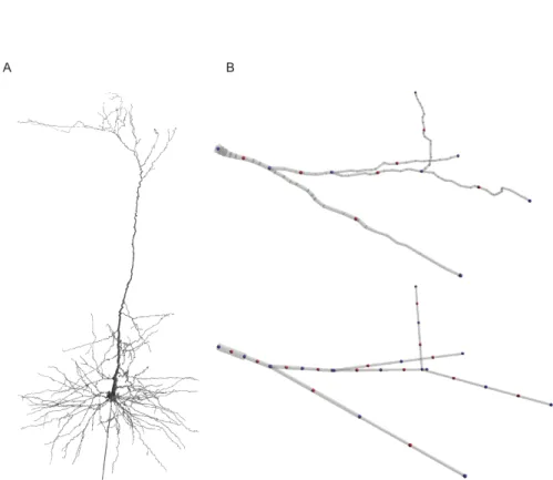
Computational models which take into account all of these aspects in-cluding active membrane conductances, realistic dendritic morphologies and complex 3D connectivity will be required to fully understand the informa-tion processing capabilities of these of brain regions (Segev and London, 2000). An example of detailed modelling closely tied to anatomical and physiological experimental data is found in Vervaeke et al (2010). This in-vestigation into electrically coupled Golgi cells used electron microscopy to
Figure 1.2: Cells from different brain regions exhibit distinct morphologies and possess different complements of active membrane conductance. Left column: CA1 pyramidal cell, with locations of conductances underlying fast Na+ (top), delayed rectifier K+ (middle) and Ih (bottom) currents. Red
indicates high density, yellow low and grey not present. Middle: Layer 5 pyramidal cell, with (from top) fast Na+ , Kv1.1 and Ih conductances.
Right: Purkinje cell, with (from top) persistent Na+ , A-type K+ and P-type Ca2+ conductances.
localise gap junctions on the cells’ dendrites, paired recordings to charac-terise the electrical coupling strength, and how it decays with inter-soma distance, and morphological reconstructions for detailed conductance based cell models. These data, together with realistic cell density information, was used to construct a 3D model of the Golgi cell network in a small patch of the cerebellar granule cell layer. This model provided valuable insights into the underlying causes of network desynchronisation by sparse synaptic input which would have been difficult to gain from experiments alone (see section 5.1.4 for more details).
1.2.3 Modelling active conductances
Even today most of the computational models of active membrane conduc-tances used for neuronal modelling rely on the formalism developed in the 1950’s by Hodgkin and Huxley. The development of this model for action potential generation in the squid giant axon (Hodgkin and Huxley, 1952) is one of the first and best examples of applying a rigorous mathematical mod-elling framework to a problem in biology and can be seen as a forerunner of much of computational biology.
Their work led to an understanding of how action potential generation and propagation is based on voltage dependent, ion selective conductances in the axon membrane. Through a series of voltage clamp experiments, they examined this voltage dependence and determined that conductances could be described in terms of a number of “gates”, which can be open or closed, all of which need to be open for current to flow. By conducting experiments in normal intracellular fluid, and with zero sodium, they isolated the be-haviours of the sodium and potassium components and found that the gates could be activating (increasing probability of being open as the membrane
becomes depolarized) or inactivating (more open at hyperpolarized poten-tials). Gate opening also showed a time dependency for getting to a steady state at a given membrane potential. The functional forms of the expres-sions for the conductance of a population of sodium (3 activating gates, m and 1 inactivating, h) and potassium (4 activating gates, n) channels (in terms of the total possible conductance, gmax, when all channels are open) are given below:
GN a(v, t) =gmaxN a·m(v, t)3·h(v, t) (1.1)
GK(v, t) =gmaxK·n(v, t)4 (1.2)
The gating variables of the Na+ channel, m and h, will be determined by the forward (closed to open,αmandαh) and reverse (open to closed,βm
and βh) transition rates (a similar relation applies for n, αn and βn):
dm(v, t)
dt =αm(v)·(1−m)−βm(v)·m (1.3) dh(v, t)
dt =αh(v)·(1−h)−βh(v)·h (1.4)
The equations for αm,βm etc. were experimentally determined to have
the following forms (using the modern convention of extracellular space at 0mV): αm(v) = 0.1·(v+ 40) 1−ev+4010 (1.5) βm(v) = 4·e v+65 −18 (1.6) αh(v) = 0.07·e v+65 −20 (1.7) βh(v) = 1 ev+35−10 + 1 (1.8)
An important point about the work of Hodgkin and Huxley is that the model was constructed to match the experimental data they had available at the time, yet the form of the model made a number of suggestions about the biophysical underpinnings of the membrane currents which have since been experimentally verified (e.g. individual membrane proteins selective to ion species containing multiple independent gating elements). This is the hallmark of a good model: it is driven by experimental data and makes predictions which can in turn be experimentally verified. Good models will survive as new experimental data accumulates, confirming their validity, bad models will be dropped. If a relatively simple model such as this can adequately approximate very complex biophysical processes (complex 3D conformational changes of large proteins embedded in the membrane) 60 years after it was first introduced, it is the sign of a very useful model indeed.
There have been many developments in the modelling of ion channels since this pioneering work, not least in terms of the computational options available for solving the equations for the model (Brette et al, 2007). While Hodgkin and Huxley had to use a hand cranked calculator to produce so-lutions to the equations, a range of neuronal simulators are available today to researchers to simulate neural networks containing hundreds of thou-sands of such cells (section 4.1.1). There have been significant developments too in terms of the biophysical description of the ion channels themselves (Destexhe and Huguenard, 2000; Hille, 2001). An important extension of the Hodgkin-Huxley model was incorporation of intracellular [Ca2+] depen-dence on gating behaviour, as found in BK and SK channels. It is also more common nowadays for ion channel physiologists to describe the multitude of states a channel can be in and the set of transition probabilities to change
between these (known as kinetic state or Markov models). These transi-tions can be complex functransi-tions of membrane potential and temperature, and depend on [Ca2+] or a number of other channel specific ligands and
computational models of channels are increasingly including these features (Destexhe and Huguenard, 2000; Graham, 2002).
Despite these advances the basic Hodgkin-Huxley formalism is still widely used in conductance based neuronal modelling. The question of how much further detail is really needed will very much depend on the question be-ing addressed with the model (Fink and Noble, 2009). Investigation of the effect of channelopathies or a specific drug interaction on the behaviour of a network will require a greater level of detail at the individual ion chan-nel level, but will lead to greater computational costs for the simulations. Standardised ways to share the information on ion channel kinetics between researchers who wish to use them in computational models have been lacking until recently.
1.2.4 Cable theory and compartmental modelling
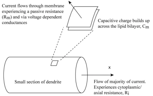
The elegant dendritic processes that most neurons possess were sadly ne-glected for many years by experimentalists as merely passive summators of synaptic input, with all of the interesting computations happening at the soma. This idea slowly began to change as researchers gained more insight into the electrical properties of dendrites and the unique computational ca-pabilities they possessed. Inspired by work investigating the propagation of electrical signals through undersea telegraph cables, researchers in the 1950s and 1960s, in particular Wilfred Rall (Rall, 1959; Rall and Agmon-Snir, 1998) started to develop models of current flow in dendrites which took into account the axial flow through the conducting cytoplasm, the ion flow
Figure 1.3: A section of a dendrite illustrating the flow of electrical current
through the membrane and the capacitive charging of the lipid bilayer. By considering these currents in small sections of the dendrites (Figure 1.3), it was possible to derive expressions for the flow of electrical current and hence the spread of membrane depolarisation in a a one dimensional dendrite in terms of these experimentally measurable quantities.
The second order partial differential equation below describes the time varying membrane potential, v, at a given point x along an infinite dendrite.
1 Ri ∂2v(x, t) ∂x2 =Cm ∂v ∂t + v Rm (1.9)
Defining the termsλ= (Rm/Ri)1/2(space constant) andτm= RmCm
(mem-brane time constant) allows the equation to be rewritten as (Rall, 1959):
λ2∂
2v(x, t)
∂x2 −τm
∂v
The concepts of the space constant (and hence the electrotonic length, physical length divided byλ) and the membrane time constant are still very relevant today. The pioneering work in this area led to many predictions for the properties of passive dendrites, including the greater attenuation of sig-nals travelling towards the soma as opposed to towards the distal dendrites, the broadening and delaying of synaptic potentials, and the basic rules of integration of distributed excitatory and inhibitory synaptic input.
While this basic formalism is sufficient to explain a number of features of passive dendrites and to provide analytical solutions to the time evolu-tion of currents in them, it is insufficient in the case where the dendrites are endowed with active voltage dependent conductances. In this case, com-partmental modelling is used (Segev and Burke, 1998), where the cell broken into isopotential compartments (Figure 1.4) and the synaptic and membrane currents into and out of each of them is calculated. This reduces the prob-lem to a set of ordinary differential equations which needs to be solved for the behaviour of the system. This has required specialised software packages and efficient algorithms (Hines, 1984) to be developed. Today, there are a number of options for developing detailed compartmental models (section 1.3.1) to investigate the complex interplay of morphology and active con-ductances underlying dendritic computation. However, each uses its own approach to solve the systems of equations and until recently it has been very difficult to test that model behaviour is independent of the choice of numerical integration method used.
Figure 1.4: Modelling of dendrites as electrically connected compartments. A) Schematic of original neuron whose electrical behaviour is to be mod-elled. B) Compartmentalisation of neuronal morphology. The cell is split into a small cylinders with dimensions based on the original cell. C) Equiv-alent circuit representation of the cell. Each compartment is modelled as a sub-circuit with a capacitance, ohmic leak current, and time varying cur-rents due to active conductances across the membrane and synaptic conduc-tances. The compartments are linked by resistances due to the cytoplasmic resistivity.
1.3
Current practices in detailed neuronal
mod-elling
Some of the key model formalisms used when creating detailed neuronal models have been discussed in the previous section. But how are these used in practice? What computational resources have been made available to the community to facilitate building and analysing such models? How much computational experience is needed to create and modify models with such packages? What happens to a model after a publication is released describing research conducted using it? Does it get reused or developed further by other parties? And how have these technical and social aspects of model development contributed to the lukewarm reception that biophysically detailed modelling often receives from experimental neuroscientists?
1.3.1 Neuronal simulators
Creating a program to simulate a network of Integrate and Fire neurons requires a relatively small amount of code (a few tens of lines of MATLAB should suffice3) and most researchers using such networks normally develop their own system from scratch, customised to their needs and preferred model structure. In contrast, simulators for conductance based neurons (beyond the classic Hodgkin-Huxley squid axon model), potentially capable of multicompartmental modelling, take longer to create and test, and devel-opment of these normally follows one of three routes: 1) The core numerical integration platform (potentially with graphics and analysis functionality) evolves into a general purpose neuronal simulation platform, of use to oth-ers outside the initial developoth-ers. Examples given below generally fall into
3
this category, with strong user communities, online documentation, and lists of publications available where the simulators are used; 2) The simulation platform is used mainly by the core set of modellers who initially created it for their own research and while it is made freely available is little used outside of that team or beyond the models it was initially developed for (e.g. Roger Traub’s FORTRAN implementation for his thalamocortical network model (Traub et al, 2005), Lyle Graham’s SurfHippo4); 3) The core simu-lation platform continues to be developed and used in ongoing research but is not made widely accessible to the community (e.g. Paul Rhodes’ simula-tion platform (Rhodes and Gray, 1994), Izhikevich thalamocortical network model (Izhikevich and Edelman, 2008), SPLIT simulator (Djurfeldt et al, 2008), Blue Brain Project infrastructure (Markram, 2006)). While this last scenario may sometimes be due to the desire to keep a competitive advan-tage over others in the field, it can also arise due to lack of time/manpower to support any other users of the system.
Thankfully, an increasing number of software packages are being made freely available to the wider community. The advantages of having multiple users testing and helping to refine a package can help make up for the extra work needed to support the software. An important part of this process is making the applications open source. Users are free to inspect the source code of the application to debug, optimise or extend the package, all of which benefits the wider user base.
Two of the most widely used packages for detailed neuronal modelling have been NEURON (Carnevale and Hines, 2006) and GENESIS (Bower and Beeman, 1997). Both of these packages support development of conductance based multicompartmental cell models and networks of neurons (of types
IV in Figure 1.1B, and sometimes type V), and have been in development for over 20 years. NEURON is still in active development with important re-cent extensions including the ability to run on parallel computing resources (Hines and Carnevale, 2008; Migliore et al, 2006). Active development of GENESIS 2 has stopped but there are important reimplementations of the core features in MOOSE (Multiscale Object Oriented Simulation Environ-ment; Ray and Bhalla (2008)) and Neurospaces/GENESIS 5 (Cornelis and De Schutter, 2003). One other recently developed simulator for multicom-partmental modelling is PSICS (Parallel Stochastic Ion Channel Simulator, Cannon et al (2010)) which allows simulation of detailed neuronal models which include stochastic ion channel transitions, and so can be used to ex-amine the effect of low numbers of ion channels on neuronal firing behaviour. Another widely used simulation platform is NEST (NEural Simulation Tool, Diesmann and Gewaltig (2002)). This platform is mainly intended for large scale networks of simplified neurons (type V in Figure 1.1B) and the continued development of it has led to much valuable research in the general principles of network simulations on parallel hardware (Morrison et al, 2005; Plesser et al, 2007). Brian (Goodman and Brette, 2008) is a Python based simulator which specialises in allowing model behaviour to be specified in simple scripts, and is actively developing methods to use these scripts to gen-erate optimised code for faster simulation, including execution on graphics processing units (GPUs) and other parallel computing hardware (Goodman, 2010). XPP (or XPPAUT, these names are used interchangeably) is a widely used tool for the analysis and simulation of generic dynamical systems, and can be used to construct a wide range of single compartment cell models (of types IV-VI in Figure 1.1B), well as small networks of these (Ermentrout,
2002).
This brief overview illustrates that there are multiple packages available for the simulation of neurons at different levels of abstraction (Brette et al, 2007). The relative strengths of each of these platforms in different techni-cal areas will determine the choice of which to use for a specific modelling task and these have been discussed in more detail elsewhere (Gleeson et al, 2010b). While the availability of a range of simulators has had many advan-tages, there have also been problems associated with this diversity (Djurfeldt and Lansner, 2007). A key issue has been that the format for the native scripts for each of the simulators are different, e.g. a cell morphology file or a channel model created for NEURON cannot be used directly by GEN-ESIS, making it difficult to reuse models and check their behaviour across simulators.
1.3.2 Model publication, dissemination and reproducibility
A key requirement for any scientific publication is that it should contain enough information for another researcher in the field to independently re-produce the described results. In cases where obtaining experimental data depends on new or specialised equipment this can be difficult in practice, but for publications focussed on modelling, giving access to the simulation scripts used is an excellent way to allow others to reproduce, critically assess and build on the results obtained in the paper.
In practice however, this is not always how things proceed. Journals (even ones focussed on computational neuroscience) generally do not re-quire release of simulation scripts when modelling results are published. This is in contrast to bioinformatics publications, which require for example
submission of microarray data in a recognised database before publication6. There is still a requirement for modelling papers to give sufficient detail to reimplement the model (e.g. large tables of ion channel kinetics, channel densities, network connectivity matrices, etc.) but in practice it is quite dif-ficult to fully reproduce the model simply from data given in the paper and supplementary information. While there has been some work on producing guidelines for information in publications on network models (Nordlie et al, 2009), there is still no substitute for freely available scripts which can be rerun to reproduce figures from a publication.
ModelDB7 (Hines et al, 2004) has been a valuable resource for those looking for scripts from publications using computational models. It con-tains a large number of neuronal models built using a range of simulators (with the NEURON simulation environment being the most popular) and it has been instrumental in convincing the community of the usefulness of providing code to accompany published models. While there are still some researchers who don’t release their modelling code after publication, the ben-efits in terms of others referencing and building on one’s work are incentive enough to convince most researchers to share their simulation code.
1.3.3 Accessibility and model reuse issues
Assuming that the scripts for a model described in a paper are available, there are still some barriers to wider reuse of a published model (or compo-nents of it, for example channels, synapses or individual cell models). With most simulators having their own proprietary scripting formats, a researcher must either use that simulator or manually convert the model to their
pre-6
A list is presented here: http://www.mged.org/Workgroups/MIAME/journals.html of journals requiring MIAME (Minimum Information About a Microarray Experiment) compliant data as a condition for publishing papers detailing microarray based results
ferred platform’s format (and so become proficient in both simulators’ native languages). Success at that endeavour usually depends on well structured and commented code, something which is not always the case. If the simu-lator is “home grown” or not widely used, even basic documentation for the simulator scripting language itself might be lacking.
Modularity of the code is needed for extracting specific components of a model, but is not always present, e.g. in MATLAB scripts where the phys-iological properties of a model might be interspersed with numerical inte-gration setting, simulation control flow, visualisation elements and analysis functions8.
These issues point to the need to develop a modular exchange format for describing the physiological components of detailed neuronal models. This should not contain any information specific to particular simulator’s implementation of the model, but just the parameters to create an instance of a model according to a shared model formalism. Also, the exchange format should not need to restate the underlying model equations each time (e.g. each channel file shouldn’t need to redefine the Hodgkin-Huxley model). The specification of the format should describe the physiological concepts sufficiently and each application should map this to/from its internal format when importing/exporting the model. In this way a researcher can choose one tool for constructing the models, choose the fastest or the one with best parallel computing support for simulating the model, and the most appropriate for visualising and analysing the results.
Reuse of models in this way has other advantages too. Testing a model on multiple simulators can remove any dependencies of the model behaviour
8
An example of this practice can be found in the following model: http://senselab.med.yale.edu/ModelDb/ShowModel.asp?model=59479; a cerebellar stellate cell model in MATLAB specifying cellular properties, channel kinetics, numerical integration and plotting of results, all in a single file but with just 3 lines of comments
on the implementation of the original simulator. This is very useful for de-bugging the models which are quite complex software systems in themselves. The more researchers who use the models means more critical eyes on the model parameters and behaviour. Researchers who wish to use model com-ponents which have been tested by multiple groups can have more confidence to use them as “black boxes” on which to build larger scale composite mod-els.
1.3.4 Biological variability versus mean model development
A common practice when creating a cell model has been to tune the model to a particular set of experimental data, e.g. the average measured physiological values (such as passive electrical properties) or spiking behaviour. This does not take account of the variability inherent in biological systems (Marder and Taylor, 2011) where a wide range of cellular behaviours can be exhibited by the cells of the same type. Similarly for network models, identical network elements are normally used and often there is no heterogeneity in the cellular or synaptic parameters.
An alternative approach to producing a single ideal model is to create populations of models, and investigate how well these models reproduce the measured ranges of behaviour of the experimental system. It has been found that models with disparate sets of parameters can reproduce target behaviour (both in the case of the conductance densities in single cell models (Golowasch et al, 2002) and when varying synaptic properties in networks (Prinz et al, 2004)). This suggests that in biological systems too there is no one ideal set of channels or synapse properties which are needed to produce a desired system behaviour.
param-eters representing “mean” model behaviour and reproduce a single aspect of the published model (e.g. one of the figures from the paper). While these “snapshots” of models are useful entities for sharing and encoding in standardised declarative formats, it is also useful to share the code for analysing them, for generating parameter searches and multiple instances of network connectivity. This is ideally done with a multi-platform, easy to learn, modern programming language, as opposed to scripts tied to the orig-inal simulation platform. Facilitating investigation of a model’s behaviour across its biological parameter space can maximise the knowledge shared when such models are made available to the community.
1.3.5 Generation and control of large scale network simula-tions
A particular set of issues arises when exchanging models whose complex-ity requires high performance computing resources to build, simulate and analyse them. While a morphologically detailed single cell model or small network can be easily run on a single processor and a graphical interface provided to plot membrane potential and other variables, managing the construction and execution of large scale networks in a parallel computing environment, and dealing with and extracting useful information from the simulation results, is usually very specific to the hardware and software in-frastructure involved. Those researchers who develop the system, set up the compute nodes and manage the simulations are often the only ones who can get full benefit from the system as a whole.
In some cases groups of researchers who develop such systems do make concious efforts to share their work with others, as in the case of the NEST
Initiative9, who make their core simulator available and have many publica-tions on the general principles of managing large scale simulapublica-tions (Morrison et al, 2005; Plesser et al, 2007). In other cases the complexity of the special-ist hardware infrastructure involved and the complex tool chain needed for the iterative development of large scale models has been used as a reason for not actively sharing software e.g. in the case of the Blue Brain Project (Markram, 2006).
In any case, there are still significant barriers to the use and analysis of such complex networks for researchers without backgrounds in software development. This is a particular concern since it is precisely investigators who have hands on experience with the physiology and anatomy of the systems in question who will be the ones who will assess how “realistic” these network models are and who will be needed to contribute their knowledge to improving the systems.
1.3.6 Testing and validation of distributed model compo-nents
When distributing software models to other researchers, (automated) test-ing of model components will also be important. How does someone who downloads a particular model know that it’s behaving as intended on their operating system, with their particular version of the simulator? If they port the model to another simulator what are the key results that need to be reproduced? While these types of tests are standard practice in software development, they are rarely used with computational neuroscience models, but inclusion of these would increase the confidence of researchers who want to reuse elements of existing models.
9
1.3.7 Comparison with Systems Biology field
The Systems Biology10field (Kitano, 2002) has been developing and sharing models of signalling pathways, metabolic and gene regulatory networks in a more organised fashion as compared to computational neuroscience for many years (De Schutter, 2008). A number of years ago the developers of some of the tools for modelling and analysing such networks came together and decided to come up with a “lingua franca” to exchange the models between their applications, and SBML (Systems Biology Markup Language) was created (Hucka et al, 2003). Now over a decade old, it is in its third major revision, there are over 200 software tools which support all or part of the language11 and there is a growing database (BioModels12) containing curated models in the format (Le Nov`ere et al, 2006), each of which can be easily validated as complying to a specified version of the language.
An initiative with similar aims, CellML (Lloyd et al, 2004), is being de-veloped by the Auckland Bioinformatics Institute and also has a number of supporting applications13 and a database of models (Lloyd et al, 2008)
with entries covering a wide range of biological phenomena. While CellML is developed by a smaller core team than SBML, it has close links with the Virtual Physiological Human project (Kohl and Noble, 2009). CellML and SBML have developed as separate initiatives but there have been efforts at technical interoperability for some time (Schilstra et al, 2006). CellML ver-sions of most of the SBML models in the BioModels database can be
down-10There are almost as many definitions of Systems Biology as there are of Computational
Neuroscience. Here I use the definition of the field which emphasises the construction and validation of computational models as a key element in a workflow of iterative refinement of models of a biological system: initial experimental data is gathered on a system, conceptual and computational models are created which lead to new predictions for the behaviour of the system, experimental verification is performed and models refined
11
http://sbml.org/SBML Software Guide
12
http://www.biomodels.net, with 366 curated models (September 2011)
13
loaded. There are also efforts at having joint meetings (and “hackathons” aimed specifically at software interoperability testing) between these and other initiatives in the field14.
A number of valuable lessons can be learned from experiences in the Systems Biology field which would increase the accessibility, interoperability and reuse of models in computational neuroscience. However, the multiple biological scales in neuronal systems (Figure 1.1), the spatially distributed nature of neuronal signalling and the host of nonlinear interactions between entities in the nervous system substantially increase the challenges for cre-ating standards for and sharing neuronal and network models.
1.4
Outline of work
To address the issues raised in the previous sections, I have been actively involved in the development of new tools to facilitate the development of complex networks of biophysically detailed neuronal models. The work was initially motivated by the need to create more detailed 3D cerebellar net-work models within the Silver Lab (Gleeson et al, 2007; Vervaeke et al, 2010), but the generally applicability of the tools and methods have led to wider interaction with the computational neuroscience community and close involvement with international efforts to improve the overall interoperability and usability of software for modelling neuronal systems. My contributions in these areas are summarised below.
14Coordinated by the COmputational Modeling in BIology NEtwork:
Software for greater accessibility of neuronal models
To facilitate the development of networks of biophysically detailed neurons, I developed the application neuroConstruct (Gleeson et al, 2007). It fea-tures a graphical user interface (GUI) to allow complex 3D networks to be constructed and visualised, supports code generation for many widely used simulators, and has inbuilt network analysis functionality. Chapter 2 discusses the motivation, design considerations and functionality of neuro-Construct in more detail.
This open source application is intended for use both by researchers without extensive programming experience for automated model generation and analysis, and for more advanced modellers who want much lower level control over model creation and simulator execution. A number of published cell and network models have been converted to neuroConstruct format and made available for users of the application. The software was publicly re-leased in 2007 and to date has had over 1,100 registered user downloads.
Contribution to standards development for biophysically realistic neuronal modelling
The multitude of simulator specific formats for creating neuronal models has been a concern of the community for many years (Brette et al, 2007; Cannon et al, 2007; Djurfeldt and Lansner, 2007). NeuroML15 has been
an initiative dedicated to developing specifications for describing models in computational neuroscience for over a decade. I became involved in this process early in my PhD and have been one of the main technical contrib-utors to the initiative since then. Version 1.x of the language focussed on describing networks of multicompartmental conductance based neuron
mod-15
els (Gleeson et al, 2010a), and was heavily influenced by efforts to generate matching simulation results on NEURON and GENESIS from code gener-ated by neuroConstruct. Over time NeuroML models could be run on other simulators in this way, and a number of other software developers have in-dependently added NeuroML support (Gleeson et al, in press). Currently there are over 20 software packages which support some part of NeuroML and others have support in their development roadmaps16.
Efforts towards NeuroML version 2.0 are also well under way. This new version will have greater flexibility in model specification for extending the language, have better support for abstract models (types V-VI in Figure 1.1B) and will allow greater interaction with languages such as SBML and CellML (allowing models to be created across scales I-VI in Figure 1.1A).
Chapter 3 describes the development of the NeuroML language, dis-cusses version 1.x in detail, outlines the tools with NeuroML support I have developed, and describes ongoing work for version 2.0 of the language.
Creation and management of large scale network simulations
The types of models which can be created with neuroConstruct and ex-changed in NeuroML format span from single compartment cell models to complex 3D microcircuits containing thousands of cells. The large scale net-works enabled by these technologies cannot be run on single processors and require interaction with high performance computing platforms. neuroCon-struct was extended to allow generation of scripts for Parallel NEURON, enabling simulation of networks on a much larger scale than previously pos-sible. This has been incorporated so that the interaction with high perfor-mance computing resources is as transparent as possible: there is minimal
16
An up to date list of all packages featuring NeuroML support is maintained here: http://www.neuroml.org/tool support
extra interaction through the GUI needed for simulations to run on remote distributed hardware as compared to running them locally.
Another valuable extension of the core neuroConstruct functionality was the addition of a scripting interface based on the Python language. This lan-guage is becoming widely used in computational neuroscience as a method of tying specialised software packages together. Providing this interface to neuroConstruct facilitates complex repetitive operations and generation of populations of models which would normally have to be done through the GUI.
Chapter 4 discusses the various additions to neuroConstruct and asso-ciated tools which I have created to facilitate management of large scale simulations.
Making key cell and network models from diverse brain regions available in standardised and accessible formats
A number of detailed cell and network models have been converted to Neu-roML format over the past number of years. These include detailed cell models from the cerebellum (De Schutter and Bower, 1994; Solinas et al, 2007a; Vervaeke et al, 2010), network models of the granule cell layer (Maex and Schutter, 1998), morphologically detailed cortical (Kole et al, 2008; Mainen et al, 1995) and hippocampal (Migliore et al, 2005) pyramidal cell models, a network model of the dentate gyrus (Santhakumar et al, 2005) and a thalamocortical network model (Traub et al, 2005) containing neu-ron models from multiple cortical layers and the thalamus. The process of converting these models has highlighted a number of issues with models developed for specific simulators and has helped to optimise the supporting simulators. The models themselves have been more thoroughly tested and
often extended beyond their original scope (e.g. network models converted to 3D). Having models in a common format has also allowed direct com-parison of models of the same cell types developed by different groups on different simulators.
Chapter 5 details the range of models which have been studied as part of this work, a number of which have been used for original scientific research within the Silver Lab (Farinella et al, 2011; Rothman et al, 2009; Vervaeke et al, 2010). These have been made available as core examples of models in NeuroML and as neuroConstruct projects and have developed and improved as these technologies move forward.
Chapter 6 summarised the main objectives of this work and evaluates the performance of the solutions presented against these. Chapter 7 discusses the work in the wider context of computational neuroscience and the ongo-ing efforts to understand the brain through a combination of experimental, theoretical and computational investigations.
Design and Implementation of
neuroConstruct
This chapter describes neuroConstruct (Gleeson et al, 2007, 2008), a mod-ular software application for the development of detailed neuronal and net-work models in 3D. It explains the motivation for developing the application, gives details on the implementation, describes the key features, and outlines the interaction of the application with the range of supported simulators and other tools.
2.1
Overview
2.1.1 Motivation for developing neuroConstruct
The main motivating factors for developing neuroConstruct have been both biological and modelling related, i.e. what are the anatomical and physio-logical aspects which need to be incorporated into the models, and what methods have been available for creating them?
Biological perspective
A wide range of information processing tasks can be carried out in complex dendritic trees endowed with active conductances. Electrical behaviour can
be very different in distinct regions of the cells, and reconstructed neuronal morphologies coupled with information on ion channel placement and ki-netics allow investigation of this. Experimentalists also need to be able to relate the behaviour of these models with the data they have recorded in real cells.
Many interesting regions of the brain have multiple cells of different types arranged in distinct 3D patterns. More experimental data is becoming available on the simultaneous behaviour of populations of cells in such areas. Models of signal flow and information processing in these networks will be of greater use for understanding neuronal function if significant details of their 3D structure can be incorporated into the models.
Neurons in many cortical regions exhibit complex connectivity patterns, with layer and cell region specific synaptic connectivity. Much of this is nonuniform, with probabilities of connection and synaptic strengths decay-ing with distance. Allowdecay-ing models to be created which incorporate such complex cells and connectivity, and which can be visually verified and anal-ysed (particularly important for models with large numbers of cells and connections) was the initial motivation for the application.
Modelling perspective
Creation of detailed cell and network models has typically involved writing scripts in a simulator specific format. These scripting languages commonly allow a mixture of model creation, execution logic, graphical elements and simulation analysis. This approach is useful for a single researcher or closely working group of modellers, but can result in quite a complex software system when the model becomes large. It also makes it difficult for other parties to reuse all or part of the model.