Time Series Analysis of Nyala Rainfall Using ARIMA Method

Time Series Analysis of Nyala Rainfall Using ARIMA Method

1_{Khartoum College of Technology, Sudan}

2_{College of Water and Environmental Engineering, Sudan University of Science and Technology (SUST)} [email protected]

Received: 11/09/2014 Accepted: 02/11/2014

ABSTRACT - This paper presents linear stochastic models known as multiplicative seasonal autoregressive integrated moving average model (SARIMA).The model is used to simulate monthly rainfall in Nyala station, Sudan. For the analysis, monthly rainfall data for the years 1971–2010 were used. The seasonality observed in Auto Correlation Function(ACF) and Partial Auto Correlation Function(PACF) plots of monthly rainfall data was removed using first order seasonal differencing prior to the development of the SARIMA model. Interestingly, the SARIMA (0,0,0)x(0,1,1)12 model developed was found to be most suitable for simulating monthly rainfall over Nyala station. This model is considered appropriate to forecast the monthly rainfall to assist decision makers to establish priorities for water demand, storage, distribution and disaster management.

Keywords: Sudan, Nyala station, rainfall, Sarima model, ACF, PACF

ﻝا صﻠﺨﺘﺴﻤ - مّدﻘُﺘ ِﺔﻗروﻝا ﻩذﻫ ﺔﻴﻓدﺎﺼﺘﻝا ﺔﻴطﺨﻝا جذﺎﻤﻨﻝا ﺔﻴﻤﺴوﻤﻝا كرﺤﺘﻤﻝا طﺴوﺘﻤﻝا ﻲﻠﻤﺎﻜﺘﻝا ﻲﺘاذﻝا رادﺤﻨﻻا جذﺎﻤﻨﺒ ﺔﻓورﻌﻤﻝا (SARIMA) . ِﺔطﺤﻤ ﻲﻓ ِيرﻬﺸﻝا ِرطﻤﻝا ةﺎﻜﺎﺤﻤﻝ ُلﻤﻌَﺘﺴُﻴ جذوﻤﻨﻝا نادوﺴﻝا ،ﻻﺎﻴﻨ . ِتاوَﻨَﺴﻠﻝ ًﺔﻴرﻬﺸﻝا ِرطﻤﻝا تﺎﻨﺎﻴﺒ ْتﻠﻤﻌﺘﺴإ ،ِلﻴﻠﺤﺘﻠﻝ 1971 -2010 . ﻲﺘاذﻝا طﺒارﺘﻝا ﺔﻝاد تﺎططﺨﻤ ﻰﻓ ﺔظﺤﻼﻤﻝا ِﺔﻴرﻬﺸﻝا ِرطﻤﻝا ِتﺎﻨﺎﻴﺒ ﻲﻓ ﺔﻴﻤﺴوﻤﻝا (ACF) ﻲﺘاذﻝا طﺒارﺘﻝا ﺔﻝاد و ﻲﺌزﺠﻝا (PACF) ﺎﻨﺎﻴﺒﻠﻝ ﻰﻤﺴوﻤﻝا ﻰﻝوﻷا ﺔﺠردﻝا نﻤ قﻴرﻔﺘﻝا مادﺨﺘﺴﺎﺒ تﻠﻴزأ جذوﻤﻨﻝا رﻴوطﺘ لﺒﻗ ت . جذوﻤﻨ نأ دﺠو ،ﻩﺎﺒﺘﻨﻸﻝ رﻴﺜﻤ لﻜﺸﺒ SARIMA(0,0,0)X(0,1,1) ِﺔطﺤﻤﻝ ِيرﻬﺸﻝا ِرطﻤﻝا ةﺎﻜﺎﺤﻤﻝ ﺔﻤﺌﻼﻤ رﺜﻜأ روطﻤﻝا . ﻻﺎﻴﻨ . ِجذوﻤﻨﻝا اذﻫ رﺒﺘﻌﻴ ِيرﻬﺸﻝا ِرطﻤﻝا ﻊﻗَوَﺘﻝ مﺌﻼﻤ رارﻘﻝا ِﻲﻌﻨﺎﺼ ةَدَﻋﺎَﺴُﻤﻝ ﻰﻓ ِءﺎﻤﻝا ِتﺎﺒﻠطﺘﻤﻝ ِتﺎﻴوﻝوﻷا سﻴﺴﺄَﺘ ) نﻴزﺨﺘ -ﺘ و ﻊﻴزو ثراوﻜ ةرادإ ( . INTRODUCTION

Sudan is one of the countries whose economy depends on rain fed agriculture associated with recurring cycles of natural drought. For many decades, recurrent drought, with intermittent severe droughts, became a normal phenomenon in Sudan. The most heavily affected areas in Sudan are Darfur and Kordofan, with 17 major droughts recorded in Darfur in the last century [1]. Drought threatens approximately twelve million hectares of rain fed land, particularly in the northern Kordofan and Darfur state[2].Severity of drought depends upon the variability of rainfall amount, as well as distribution and frequency. Rainfall is the most important climatic element that influences agriculture. Monthly rainfall forecasting plays an important role in the planning and management of agricultural scheme and water resources systems. The main objective of the present study is to

develop a valid stochastic model to simulate monthly rainfall in Nyala region.

Rainfall is a seasonal phenomenon with twelve months period.Seasonal time series are often modeled by SARIMA techniques. Recently, a few researchers modeled monthly rainfall using SARIMA methods. Nimarla and Sundaram[3] fitted a SARIMA (0,1, 1)x(0,1,1)12 model to monthly rainfall in Tamilnadu, India. Etuk and Mohamed [4] fitted a SARIMA (0,0,0)x(0,1,1)12 model to monthly rainfall in Gadaref, Sudan. In this study, linear stochastic models known as multiplicative seasonal autoregressive integrated moving average (SARIMA) models were used to model monthly rainfall in Nyala station, southern Darfur.

STUDY AREA

Darfur State has an area of about 490,000 km2 and lies between latitudes 10º and 20º N and

longitudes 22º and 27º E. The topography of the state is characterized by almost level or gently undulating plateau, with elevations ranging from 600 to 900 meters above sea level. The main water resources in Darfur State are the rainfall, groundwater, and seasonal khors. The rainfall decreases from South to North. The decrease in rainfall is associated with increased evaporation. The temperatures also increase in variability, and reach substantially higher levels. Rainfall varies from year to year. This variation is crucial for rain fed farming. Water scarcity is one of the main causes of tension in the state. Darfur states are one of the biggest and environmentally most varied regions of the Sudan. The region is divided into four ecological zones based on the amount of rainfall and vegetation types[5]. These zones, from North to South, are desert, semi-desert, low woodland savanna and high woodland savanna. Nyala station, Figure 1, is characterized by annual rainfall (197- 626 mm) during the last four decades. The annual number of rainy days, (rainfall > 1 mm), is 95 days and the mean annual reference potential evapotranspiration (ETo) using Penman / Monteith criterion for the station is about 2305mm[6].The climate in the Nyala is semi-arid with mean annual temperature near 26.9o C [7].

The urban economy of Nyala has been strongly associated with the rural economy of South Darfur, the most productive Darfur State [8]. As a trading centre it has also benefited from its strategic location, close to served by a railway and an international airport. Groundnuts, gum Arabic, millet, sorghum and sesame are South Darfur State main agricultural products. Along with livestock these have been its main exports, and also the base for much of Nyala’s manufacturing industry.

DATA COLLECTION

For this study, Nyala rainfall gauge was considered and 480 monthly rainfall data was procured for the period from 1971 to 2010. The monthly rainfall records for Nyala station show most of the rain falls in the period from May to October, and reaches its peak in August.

MODELING BY SARIMA METHODS

For more than half a century, Box–Jenkins ARIMA linear models have dominated many areas of time series forecasting. Autoregressive (AR) models can be effectively coupled with moving

average (MA) models to form a general and useful class of time series models called autoregressive moving average (ARMA) models. In ARMA model the current value of the time series is expressed as a linear aggregate of p previous values and a weighted sum of q previous deviations (original value minus fitted value of previous data) plus a random parameter [9]. However, an ARMA model can be used when the data are stationary. ARMA models can be extended to non-stationary series by allowing differencing of data series. These models are called autoregressive integrated moving average (ARIMA) models [10]. A time series is said to be stationary if it has constant mean and variance. The general non-seasonal ARIMA model is AR to order p and MA to order q and operates on dth difference of the time series; thus a model of the ARIMA family is classified by three parameters (p, d, q) that can have zero or positive integral values. The general non-seasonal ARIMA model may be written as

߶ሺܤሻ∇ௗܺ_௧ =ߠሺܤሻߝ_௧

where:߶ሺܤሻand ߠሺܤሻ = Polynomials of order p

and q, respectively.

߶ሺܤሻ=ሺ1 −߶_ଵܤ−߶_ଶܤଶ− ⋯߶_௉ܤ௣ሻ

And

ߠሺܤሻ=൫1 −ߠ

ଵܤ−ߠଶܤଶ− ⋯ߠ௤ܤ௤൯

Figure 1: Map of Sudan showing Nyala Often time series possess a seasonal component that repeats every s observations. For monthly observations s = 12 (12 in 1 year), for quarterly observations s = 4 (4 in 1 year). Box et al. [11] have generalized the ARIMA model to deal with seasonality, and define a general multiplicative seasonal ARIMA model, which are commonly known as SARIMA models. In short notation the

SARIMA model described as ARIMA (p, d, q) x

(P, D, Q) s, which is mentioned below:

߶௣ሺܤሻΦ௣ሺܤ௦ሻ∇ௗ∇௦஽ሺܼ௧ሻ=ߠ௤ሺܤሻΘொሺBୱሻߝ୲ Where p is the order of non-seasonal autoregression, d the number of regular differencing, q the order of nonseasonal MA, P the order of seasonal autoregression, D the number of seasonal differencing, Q the order of seasonal MA,

s is the length of season, Φ

௣and Θொare the seasonal polynomials of order P and Q, respectively. In this work the statistical and econometric software Eviews-6 was used for all analytical work. It is based on the least squares optimization criterion.

RESULTS AND DISCUSSIONS

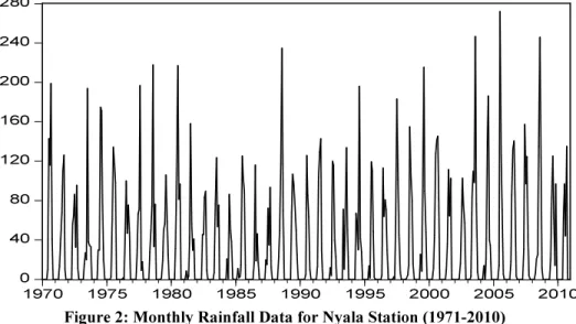
Time series plot was conducted using the monthly rainfall data for Nyala station to assess the stability of the data, and Figure 2 was obtained. Since the data is a monthly rainfall, Figure 2, shows thatthere is aseasonal cycle of the series and the series is not stationary. The seasonal fluctuations occur every 12 month, resulting in period of time series S =12. The time-plot shows no noticeable trend.

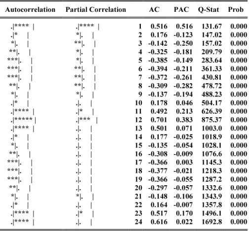
Non-stationary is confirmed by the Augmented Dickey- Fuller Unit Root Test (ADF) on the monthly rainfall data. The ADF Test was done on the entire rainfall data. Table I displays results of the test: statistic value -1.2517 greater than critical vales -2.5697, -1.9414, -1.6162 all at 1%, 5%, and 10% respectively. The ACF illustrated in Table II, also, shows clearly that the series is not stationary.

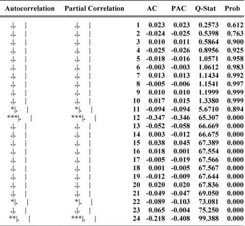
If there is seasonality and no trend takes a difference of lag S=12, this occurs because it is a monthly data with seasonality. The monthly rainfall data was differenced by one seasonal degree of differencing to achieve stationary, as shown in Table III. Augmented Dickey-Fuller Unit Root Test was done again on the seasonally differenced rainfall data (deseasonalized data). The results of the test: statistic value-7.7919less than critical vales -2.5700, -1.9415, -1.6162 all at 1%, 5%, and 10% respectively. This indicates that the series are stationary and confirms that the rainfall data needed to be differenced to be stationary.

In this step, the model that seems to represent the behaviour of the series is searched, by the means of autocorrelation function (ACF) and partial auto correlation function (PACF), for further investigation and parameter estimation. The behaviour of ACF and PACF is to see whether the series is stationary or not.For modelling by ACF and PACF methods, examination of values relative to auto regression and moving average were made. An appropriate model for estimation of monthly rainfall for Nyala station was finally found. Many models for Nyala station, according to the ACF and PACF of the data, were examined to determine the best model. The model that gives the minimum Akaike Information Criterion (AIC) is selected as best fit model, as shown in Table IV. Obviously, model SARIMA (0,0,0)x(0,1,1)12 has the smallest values of AIC and then one would temporarily have a model SARIMA (0,0,0) x (0,1,1)12 .

Figure 2: Monthly Rainfall Data for Nyala Station (1971-2010)

0 40 80 120 160 200 240 280 1970 1975 1980 1985 1990 1995 2000 2005 2010

Table I: ACF and PACF Plots For Nyala Station Monthly Rainfall Series

Autocorrelation Partial Correlation AC PAC Q-Stat Prob

.|**** | .|**** | 1 0.516 0.516 131.67 0.000 .|* | *|. | 2 0.176 -0.123 147.02 0.000 *|. | **|. | 3 -0.142 -0.250 157.02 0.000 **|. | *|. | 4 -0.325 -0.181 209.79 0.000 ***|. | *|. | 5 -0.385 -0.149 283.64 0.000 ***|. | **|. | 6 -0.394 -0.211 361.33 0.000 ***|. | **|. | 7 -0.372 -0.261 430.81 0.000 **|. | **|. | 8 -0.309 -0.282 478.72 0.000 *|. | *|. | 9 -0.137 -0.194 488.23 0.000 .|* | .|. | 10 0.178 0.046 504.17 0.000 .|**** | .|* | 11 0.492 0.213 626.39 0.000 .|***** | .|*** | 12 0.701 0.383 875.37 0.000 .|**** | .|. | 13 0.501 0.071 1003.0 0.000 .|* | .|. | 14 0.177 -0.025 1018.9 0.000 *|. | .|. | 15 -0.135 -0.054 1028.1 0.000 **|. | .|. | 16 -0.308 -0.009 1076.6 0.000 ***|. | .|. | 17 -0.366 0.003 1145.3 0.000 ***|. | .|. | 18 -0.377 -0.021 1218.3 0.000 ***|. | .|. | 19 -0.366 -0.055 1287.2 0.000 **|. | .|. | 20 -0.297 -0.057 1332.6 0.000 *|. | *|. | 21 -0.148 -0.106 1343.9 0.000 .|* | .|. | 22 0.164 -0.007 1357.8 0.000 .|**** | .|* | 23 0.517 0.170 1496.1 0.000 .|**** | .|. | 24 0.616 0.022 1692.8 0.000

Table II: ADF- Unit Root Test for Nyala Monthly Rainfall Statio

n Variable ADF test

Level of

Confidence Critical Value Probability Result

Nyala Monthly Rainfall -1.2517 1% -2.5697 0.1939 Non-stationary 5% -1.9414 10% -1.6162

Table III: Comparison of AIC for the Selected Model

Variable Station Model AIC

Monthly Rainfall Nyala

SARIMA(0.0.0)(0.1.1) 9.572 SARIMA(0.0.1)(0.1.1) 9.747 SARIMA(0.0.1)(2.1.1) 9.669 SARIMA(0.0.0)(1.1.1) 9.577 After the identification of the model using the

AIC criteria, estimation of parameters was conducted. The values of the parameters are shown in Table IV. The result indicated that the parameters are significant since their p-values are smaller than 0.05 and should be retained in the model. SARIMA. All validation tests were carried out on the residual series. The ACF and PACF of

residuals of the model SARIMA (0, 0, 0) x(0, 1, 1)12 are shown in Table V.

As shown in Table V, most of the values of the RACF and RPACF lies within confidence limits except very few individual correlations appear larger compared with the confidence limits. The figures indicate no significant correlation between residuals.

The model verification is concerned with checking the residuals of the model to see if

they contain any systematic pattern which still can be removed to improve the chosen the Ljung-Box Q-statistic is employed for checking independence of residual. From Table VI, one can observe that the p-value is greater than 0.05 for all lags, which implies that the white noise hypothesis is not rejected. The Breusch-Godfrey Serial Correlation LM test accepts the hypothesis of no serial correlation in the residuals, as shown in Table VII. The Q-statistic and the LM test both

indicated that the residuals are none correlated and the model can be used. Since the coefficients of the residual plots of ACF and PACF are lying within the confidence limits, the fit is good and the error obtained through this model, (1971-2010), is tabulated in the Table VIII. Finally, this concludes that SARIMA (0,0,0) x(0,1,1)12 model identified previously is adequate to represent the monthly rainfall data and could be used to forecast the upcoming rainfall data.

Table IV: ACF and PACF Plots for Nyala Station afterone seasonal difference

Autocorrelation Partial Correlation AC PAC Q-Stat Prob

.|. | .|. | 1 0.023 0.023 0.2573 0.612 .|. | .|. | 2 -0.024 -0.025 0.5398 0.763 .|. | .|. | 3 0.010 0.011 0.5864 0.900 .|. | .|. | 4 -0.025 -0.026 0.8956 0.925 .|. | .|. | 5 -0.018 -0.016 1.0571 0.958 .|. | .|. | 6 -0.003 -0.003 1.0612 0.983 .|. | .|. | 7 0.013 0.013 1.1434 0.992 .|. | .|. | 8 -0.005 -0.006 1.1541 0.997 .|. | .|. | 9 0.010 0.010 1.1999 0.999 .|. | .|. | 10 0.017 0.015 1.3380 0.999 *|. | *|. | 11 -0.094 -0.094 5.6710 0.894 ***|. | ***|. | 12 -0.347 -0.346 65.307 0.000 .|. | .|. | 13 -0.052 -0.058 66.669 0.000 .|. | .|. | 14 0.003 -0.012 66.675 0.000 .|. | .|. | 15 0.038 0.045 67.389 0.000 .|. | .|. | 16 0.018 0.001 67.554 0.000 .|. | .|. | 17 -0.005 -0.019 67.566 0.000 .|. | .|. | 18 0.001 -0.005 67.567 0.000 .|. | .|. | 19 -0.012 -0.009 67.644 0.000 .|. | .|. | 20 0.020 0.020 67.836 0.000 .|. | .|. | 21 -0.049 -0.047 69.050 0.000 *|. | *|. | 22 -0.089 -0.103 73.081 0.000 .|. | .|. | 23 0.065 -0.004 75.250 0.000 **|. | ***|. | 24 -0.218 -0.408 99.388 0.000

Table V: Summary of Parameter Estimates and Selection Criteria (AIC) for Nyala Monthly Rainfall

Variable Coefficient Std. Error t-Statistic Prob.

MA(12) -0.949281 0.014215 -66.77889 0.0000

R-squared 0.426765 Mean dependent var -0.355208

Adjusted R-squared 0.426765 S.D. dependent var 38.25668 S.E. of regression 28.96502 Akaike info criterion 9.572136 Sum squared resid 401867.7 Schwarz criterion 9.580831 Log likelihood -2296.313 Hannan-Quinn criter. 9.575554 Durbin-Watson stat 2.062543

Inverted MA Roots 1.00 .86-.50i .86+.50i .50+.86i

.50-.86i .00+1.00i -.00-1.00i -.50+.86i -.50-.86i -.86+.50i -.86-.50i -1.00

Table VI: ACF and PACF Plots of SARIMA (0, 0, 0)x(0, 1, 1) Residuals

Autocorrelation Partial Correlation AC PAC Q-Stat Prob

.|. | .|. | 1 -0.032 -0.032 0.4948 .|. | .|. | 2 0.007 0.006 0.5167 0.472 .|. | .|. | 3 0.029 0.030 0.9300 0.628 .|. | .|. | 4 -0.028 -0.026 1.3174 0.725 .|. | .|. | 5 -0.015 -0.017 1.4297 0.839 .|. | .|. | 6 -0.010 -0.012 1.4792 0.915 .|. | .|. | 7 0.004 0.006 1.4888 0.960 .|. | .|. | 8 -0.007 -0.006 1.5108 0.982 .|. | .|. | 9 -0.006 -0.007 1.5282 0.992 .|. | .|. | 10 0.024 0.023 1.8207 0.994 *|. | *|. | 11 -0.080 -0.078 4.9642 0.894 .|* | .|* | 12 0.080 0.075 8.0961 0.705 .|. | .|. | 13 -0.011 -0.008 8.1586 0.773 .|. | .|. | 14 0.052 0.057 9.4887 0.735 .|. | .|. | 15 0.038 0.033 10.193 0.748 .|. | .|. | 16 -0.006 -0.002 10.211 0.806 .|. | .|. | 17 -0.003 -0.006 10.215 0.855 .|. | .|. | 18 -0.000 0.002 10.215 0.894 .|. | .|. | 19 -0.005 -0.003 10.229 0.924 .|. | .|. | 20 0.011 0.012 10.287 0.946 .|. | .|. | 21 -0.041 -0.037 11.143 0.942 .|. | .|. | 22 -0.013 -0.025 11.232 0.958 .|. | .|. | 23 0.060 0.073 13.038 0.932 *|. | *|. | 24 -0.157 -0.164 25.480 0.326

Table VII: The Breusch-Godfrey Serial Correlation LM test

F-statistic 0.244495 Prob. F(2,477) 0.7832

Obs*R-squared 0.151221 Prob. Chi-Square(2) 0.9272 F-statistic 0.662316 Prob. F(12,467) 0.7879 Obs*R-squared 7.697345 Prob. Chi-Square(12) 0.8083

Table VIII: Errors Measures Obtained for the Selected Model

Error Measure Value

RMSE 29.20

MAE 15.16

CONCLUSION

It may be concluded that the monthly rainfall in Nyala, Sudan follows a SARIMA (0,0, 0)x(0,0,1)12 model. This model is considered appropriate to predict the monthly rainfall for the upcoming years to assist decision makers establish priorities for water demand, storage and distribution

REFERENCES

[1]Sharaky, A, M, (2005): OIL, Water, Minerals, and the Crisis in Darfur, Sudan.

Institute of African Research and Studies, Cairo University.

[2]Zakieldeen, S. A., (2009): Adaptation to Climate Change: A Vulnerability Assessment for Sudan. International Institute for Environment and Development, London. [3]Nirmala M, Sundaram S.M, (2010). A Seasonal Arima Model for Forecasting monthly rainfall in Tamilnadu. National Journal on Advances in Building Sciences and Mechanics, 1(2): 43 – 47.

[4]Etuk, E.H., Mohamed T.M., (2014). Time Series Analysis of Monthly Rainfall data for the Gadaref rainfall station, Sudan, by SARIMA Methods. International Journal of

Scientific Research in Knowledge, 2(7), pp. 320-327.

[5]Catterson, T.E., et al (2003), Environmental threats and opportunities assessment, USAID integration strategic plan in the Sudan 2003 – 2005, Washington, 146p. [6]LeHouérou, H.N. (2009): Bioclimatology and Biogeography of Africa. Verlag Berlin Heidelberg, Germany.

[7]Elagib, N.A., Mansell, M.G. (2000). Recent trends and anomalies in mean seasonal and annual temperatures overSudan. Journal of Arid Environments, 45(3): 263 – 288.

[8]Smith, M, B, et al., (2011): City limits: urbanization and vulnerability in Sudan, Nyala case study. Humanitarian Policy Group

Overseas Development Institute, London, United Kingdom.

[9]Mishra, A. K., Desai, V. R., (2005), Drought Forecasting Using Stochastic Models. Stochastic Environmental Research and Risk Assessment, 19(5): 326-339.

[10] Durdu, O.F., (2010), Application of Linear Stochastic Models For Drought Forecasting in The Buyuk Menderes River Basin, Western Turkey, Stochastic Environmental Research and Risk Assessment,doi:10.1007/s00477-010-0366-3. [11] Box, G.E.P., Jenkins, G.M., and Reissel, G.C., (1994). Time Series Analysis Forecasting and Control, 3rd edition. Prentice Hall.USA.