Cosigners As Collateral

Cosigners As Collateral

Stefan Klonner, Goethe Universität Frankfurt Ashok S. Rai, Williams College

Abstract: We investigate the role of cosigners as collateral using data from a South Indian …nancial institution. Our identi…cation is based on a rule of thumb that allows loan o¢ cers to discontinuously relax the cosigner requirement based on the duration of

the loan repayment. We establish a negative causal e¤ ect of cosigners on defaults. A reduction in the number of cosigners by about one-third increases the incidence of default

by 10percent for loans that are repaid over 12months relative to similar loans that repaid over13 months. Our results suggest that cosigners induce borrowers to repay.

JEL Codes: O16, D82, G21

Keywords: credit, default, cosigner, rosca

0_{We thank Bill Gentry, Michael Gordy, Wilbert van der Klaauw, Dilip Mookherjee, David McKenzie,}

Jeremy Tobacman, Tara Watson and seminar participants at Boston University, Frankfurt, Indian School of Business, Namur, NEUDC, Williams, World Bank, and Yale for helpful comments, and Martin Rotemberg for research assistance. We are grateful to the …nancial institution (in South India) for sharing their data and their time. All errors are our own.

Klonner: Grüneburgplatz 1, J. W. Goethe Universität, 60054 Frankfurt am Main, Germany. Phone

+49+69+7 98-34795, [email protected]

1

Introduction

The lack of collateral – and the accompanying …nancial constraints on entrepreneurship – are thought to be a primary cause of underdevelopment (Banerjee 2003, Townsend1997). When borrowers have no collateral of their own, lenders can ask for cosigners to pledge collateral instead. Such cosigned loans are extremely common.1 In this paper we ask if

cosigners induce borrowers to repay.

The di¢ culty with identifying the in‡uence of cosigners on repayment arises from an information asymmetry between the researcher and the lender. Lenders often have "soft"

information about the riskiness of particular borrowers – and this information is not ob-served by the researcher (Petersen and Rajan 1994, Uzzi and Lancaster 2003). A lender will typically ask riskier borrowers to pledge more collateral (provide more cosigners) based on this soft information, leading to a positive correlation between cosigners and default

rates.2 Such a positive correlation may very well mask the causal link between cosigners and default rates. For identi…cation we need some variation in cosigners assigned to similar

loans that is exogenous to the lender’s soft information on the borrower.

We use data from a non-bank …nancial institution in South India which organizes Roscas

(Rotating Savings and Credit Associations). In these Roscas, participants pledge to make monthly contributions and bid to receive the collected savings. Unlike traditional Roscas

(Besley, Coate and Loury1993), the participants in these Roscas do not enforce repayments from each other. The organizer takes on the default risk that Rosca winners may fail to make

subsequent contributions –and requires Rosca winners to pledge cosigners as collateral. Our identi…cation strategy is based on a discontinuity in the organizer’s rules. Borrowers

1

Cosigned loans are popular in the United States (Berger and Udell, 1998), in Europe (Pozzolo, 2004)

and in many developing countries. There are also numerous historical accounts of this lending practice

(Baker, 1977; Guinnane, 1994; Newton, 2000; Phillips and Mushinski, 2001).

2_{A positive correlation between traditional collateral and defaults has been found in a variety of} de-veloped and less dede-veloped …nancial markets (Berger and Udell, 1990; Jimenez, Salas and Saurina 2006). Though most theory suggests that increases in traditional collateral will reduce defaults, there has been little investigation of this causal link.

with repayments for12months or less are allowed fewer cosigners than borrowers with longer repayment durations. We compare borrowers who di¤er in their repayment durations

and hence in their cosigner requirements despite having otherwise similar loan terms. In particular, there is a reduction in the number of cosigners by about one-third for loans that

are repaid over12months relative to similar loans that repaid over13months. We …nd that this relaxation increases the incidence of default by 10 percent for those borrowers with12

month loans relative to those with13month loans holding other loan terms constant. This cosigner requirement is relaxed only for the subset of borrowers whom the organizer does

not screen directly. For the remaining borrowers, who are screened through an occupation (and income)-veri…cation process, the cosigner requirement is not relaxed and there is no

increase in default rates.

The organizer …rst attempts to collect repayments directly from the borrower – and if

that fails, goes through a long legal process to collect payments from the cosigners. We measure default rates before the organizer has collected repayments from the cosigners

thereby isolating the in‡uence of cosigners on the borrower’s repayment. Our results therefore imply that additional cosigners do more than simply provide a way to collect

funds after the loan has been defaulted on by the borrower. Put di¤erently, we reject the null hypothesis that cosigners serve only as a hedge against default risk in favor of the alternative that they promote repayment by the borrower.

Our results are consistent with several theories of cosigning. Cosigners may improve

repayment by the borrower herself by solving adverse selection problems (Besanko and Thakor, 1987) and/or moral hazard problems (Banerjee, Besley, Guinnane, 1994) just as traditional collateral does. Riskier borrowers may be attracted to the12month loans with lower cosigner requirements than safer borrower types. Alternatively, borrowers who take

the12month loans with fewer cosigners may take on riskier projects or expend less e¤ort on ensuring project success relative to those borrowers with more cosigners. Further, unlike

traditional collateral, cosigners may also promote repayment by providing a borrower with insurance if she experiences a shock (Rai and Sjöström, 2004). In all three cases (adverse

selection, moral hazard and insurance), we would expect an increase in defaults for loans with lower cosigner requirements.

Since we identify the e¤ectiveness of cosigners in promoting repayment by using a dis-continuity in the cosigner requirement at a loan-duration-threshold, the methods developed

for regression-discontinuity (RD) design seem the natural …t. The variable that determines treatment in our context, loan duration, is discrete and so any RD estimation must be

parametric. Lee and Card (2008) suggest an econometric procedure to account for the un-certainty in parametrization for such RD designs –and we follow their procedure. There is

one important di¤erence between our approach and RD design, however. In an RD design, there should be no incentive to sort around the treatment threshold, while in our context,

there is an incentive for riskier types of borrowers to choose shorter-duration loans with fewer cosigners. While the incentive to sort around the treatment threshold is a nuisance

in RD design, the role of cosigners in inducing borrowers to self-select around the threshold is precisely what this study intends to capture. So while we utilize aspects of the RD

methodology, our empirical estimates include the selection e¤ects of cosigning.

We contribute to a empirical debate on "social collateral", i.e. the use of local

infor-mation and enforcement to induce repayment among borrowers who have no traditional collateral of their own. Cosigned loans are related to group loans popular in micro…nance

(Bond and Rai, 2008): both types of lending are based on the use of social collateral to promote repayment. The cosigner in a typical cosigned loan is typically a non-borrower; a

group of borrowers cosign each other’s loans in a group loan. There is substantial debate about the e¤ectiveness of social collateral in group loans. For instance, Gine and Karlan

(2008) …nd that some circumstances where group loans are no more e¤ective at reducing defaults than individual loans. One reason why social collateral may be e¤ective in our

study but not in Gine and Karlan (2008) is that the latter abstract from selection – and hence cannot address the role of social collateral in selecting safer borrowers. Recent

empirical work has also investigated if the strength of social connectedness reduces default rates in group loans (Ahlin and Townsend 2007, Karlan2007;Wydick1999). In contrast,

our paper can be seen as investigating if the quantity of social collateral, as measured by the number of cosigners, reduces defaults. We do not have data nor exogenous variation

on the social ties between the cosigner and borrower.

Plan for the Paper

The paper proceeds as follows. In Section 2 we provide background on the non-bank …nancial institution in South India and on our dataset. In Section 3 we outline our empirical

strategy. We discuss our results in Section 4 and conclude in Section 5.

2

Data and Institutional Background

This study uses data on Rotating Savings and Credit Associations (commonly referred to

as Roscas). Roscas match borrowers and savers but do so quite di¤erently from banks. In this section we provide some background on how the Roscas in our study operate. We

pay particular attention to who holds the default risk and how loans are secured by the salaries of cosigners. We also describe the sample of Rosca borrowers that we will use in

our subsequent empirical analysis.

Rules

Roscas are …nancial institutions in which the accumulated savings are rotated among par-ticipants. Participants in a Rosca meet at regular intervals, contribute into a "pot" and

rotate the accumulated contributions. So there are always as many Rosca members as meetings. In random Roscas, the pot is allocated by lottery and in bidding Roscas the pot

is allocated by an auction at each meeting. Our study uses data on the latter.

In the bidding Roscas we study participants contribute a …xed amount to a pot every

month. They then bid to receive the pot in an oral ascending bid auction where previous winners are not eligible to bid. The highest bidder receives the pot of money less the winning bid and the winning bid is distributed among all the members as an interest dividend. The

winning bid can be thought of as the price of capital: higher winning bids imply smaller loans and higher interest rates. Over time, the winning bid falls as the duration for

which the loan is taken diminishes. In the last month, there is no auction as only one Rosca participant is eligible to receive the pot. We illustrate these rules with a numerical

example:

Example (Bidding and Payo¤s) Consider a 3 person Rosca which meets once a month and each participant contributes $10: The pot thus equals $30. Suppose the winning bid is $12in the …rst month. Each participant receives a dividend of $4: The recip-ient of the …rst pot e¤ ectively has a net gain of $12(i.e. the pot less the bid plus the dividend less the contribution, 30 12 + 4 10). In the second month, when there are 2eligible bidders, suppose the winning bid is $6: And in the …nal month, there is only one eligible bidder and so the winning bid is zero: The net gains and contributions are depicted as:

Month 1 2 3

Winning bid 12 6 0 First Recipient’s Net Payo¤ 12 -8 -10 Second Recipient’s Net Payo¤ -6 16 -10 Last Recipient’s Net Payo¤ -6 -8 20

The …rst recipient is a borrower: he receives $12and repays $8and $10in subsequent months, which implies a 30% monthly interest rate. The last recipient is a saver: she saves $6 for 2 months and $8for a month and receives $20, which implies a 67% monthly rate. The intermediate recipient is partially a saver and partially a borrower.

In what follows, we shall often refer to the winning bid or the "repayment burden" relative to the pot size. The winning bid in the above example in round 1 is $12 or 40

percent of the pot size. We de…ne the repayment burden as the total repayment owed (i.e.

the sum of contributions less dividends for a Rosca winner). The repayment burden for the round1borrower in the above example is$18or three-…fth of the pot. The repayment

burden for round 2 winner is $10 or one-third of the pot. We calculate the default rate as the fraction of the repayment burden that is overdue at the end of the Rosca. So, for

instance, if the Rosca borrower in round1failed to make his round3repayment of$10(but did make the round2 repayment of$8), his default rate would be 10₁₈ or56 percent.

The Sample

The bidding Roscas we study are large scale and organized commercially by a non-bank

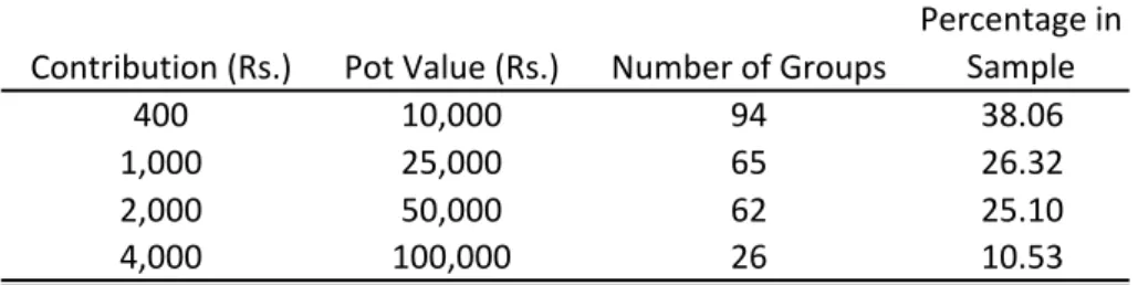
…nancial …rm. The data we use is from the internal records of an established Rosca organizer in the southern Indian state of Tamil Nadu.3 Our sample consists of all Rosca groups of

25month duration that were started in 2001: There were 247such Roscas started in2001

at four di¤erent contribution levels. Of these, the most common were those with a Rs. 400

monthly contribution and pot size of 25 400 = Rs. 10;000: We shall refer to the four di¤erent contribution levels (Rs. 400;1000;2000and 4000)as the denominations of Roscas in our sample.

In these bidding Roscas participants do not have social ties in contrast with the

person-alized Roscas studied elsewhere. The …rm that organizes the Roscas takes on the default risk. If a participant fails to make a contribution, the organizer will contribute funds on

his/her behalf. In this way, a round 18 borrower who fails to contribute in round 19 will not reduce the pot available to the other Rosca participants in round 19: In exchange the organizer receives a commission of6percent of the pot in each round. The Rosca organizer is also a special Rosca member who receives the entire …rst pot (at a zero bid) and makes contributions thereafter.

Every Rosca participant (other than the …rst and last winner) acts as both a borrower and a saver. For instance, the round 18 winner contributes for 17 months, takes a loan,

3_{Bidding Roscas are a signi…cant source of …nance in South India, where they are called chit funds.} Deposits in regulated bidding Roscas were12:5%of bank credit in the state of Tamil Nadu and25%of bank credit in the state of Kerala in the1990s, and have been growing rapidly (Vaidyanathan and Shriram,2000). There is also a substantial unregulated chit fund sector.

and then repays for the remaining 8 months of the Rosca. In what follows, however, we shall refer to the observations in our sample as Rosca borrowers to focus attention on

their repayment risk. The round18 borrower will have a lower repayment burden (sum of contributions due net of dividends from rounds19 to25)than, say, a round5 borrower.

Each observation in our sample refers to a borrower, i.e. the winner of a Rosca auction, in one of the 25 month Roscas that were started in 2001. We exclude Rosca winners in the …rst round and in the last two rounds (rounds24and 25)from our sample of borrowers since they have no repayment risk. Clearly the …rst round winner, the organizer, cannot

default on itself. The last round winner has no repayment burden (no future contributions due). The penultimate round winner has one repayment due but in practice this repayment

is deducted from the sum awarded.

Descriptive statistics for the 5434Rosca borrowers in our sample are in Table 2. The winning bid is 16:2 percent of the pot on average for these borrowers representing the fraction of the pot that the borrower is willing to forego to other participants in order to

borrow. The repayment burden or the total undiscounted outstanding repayments is46:7

percent of the pot on average. Precisely half the borrowers win pots in the second half of

the Rosca (i.e. on or after round13): The dummy variable late round indicates whether a Rosca borrower took a loan in the second half.

Defaults refer to overdues at the maturity of the loan (at the end of the Rosca). 61:4

percent of the borrowers had non-zero overdues – and this dummy variable measure is

referred to as default incidence in what follows. The default rate for each Rosca borrower is calculated as the amount outstanding at the end of the Rosca as a fraction of the repayment

burden. The mean default rate in our sample is10:3 percent (Table2).4

4_{We are interested in defaults (or missed contributions) for Rosca participants after they have won the}

pot. In some cases Rosca participants may drop out before winning the pot because they fail to make

Cosigners and Enforcement

As we have mentioned above, the …rm that organizes the Roscas takes on the risk of default. Rather than asking for physical collateral, the organizer requires auction winners to provide

cosigners before releasing the loans. Cosigners are required to be salaried employees with a minimum monthly income that depends on the Rosca denomination5. This is because

the organizer has a legally enforceable claim against their future income as collateral for the loan.

The loan o¢ cer who is an employee of the …rm that organizes the Roscas, typically has

some discretion in deciding on the number of cosigners required for each loan. In the middle round of each Rosca, however, the cosigner requirement is subject to a guideline issued

publicly by the head o¢ ce of the …rm that organizes the Roscas to all Rosca participants. This guideline stipulates a relaxation of the cosigner requirement in the middle round. It

states that Rosca borrowers will be required three cosigners for winners of auctions up to the middle round of a Rosca, but only two cosigners for winners of later auctions. The

rationale is that later borrowers have fewer contributions due and hence are lower risks than earlier borrowers. Loan o¢ cers told us that they do not view this guideline as

hard-and-fast. Instead, they see it as a "rule of thumb" that allows them to relax the cosigner requirement for borrowers in the second half of the Rosca relative to borrowers in the …rst

half.

We use three measures of the cosigner requirement to adequately capture the guidelines

issued to loan o¢ cers: the number of cosigners, the incidence of one or more cosigners, and the incidence of three or more cosigners. The average number of cosigners attached

to a loan in our sample is 0:717 with considerable variation (Table 2): 38 percent of the borrowers have one or more cosigners – and 10:5 percent had three or more cosigners. If the guideline was followed to the letter then exactly half the borrowers would have three or

5_{We did not have access to cosigner salaries – a variable which would have given us a better measure of} the "total" collateral pledged by cosigners. We return to this issue when we interpret our results in Section

more cosigners. In section 4 we shall show that the guideline is indeed followed in spirit for a subgroup of borrowers, i.e. the cosigner requirement is relaxed for round13borrowers relative to round 12borrowers.

The loan o¢ cer may also verify the auction winner’s income before releasing the loan.

For instance, a self-employed person will be asked for tax returns or bank statements while a salaried employee will be asked for an earning record. This veri…cation occurs in 29:4

percent of the cases (see Table 2): Veri…cation is a form of costly screening on the part of the loan o¢ cer – because it takes time and e¤ort. In e¤ect, loan o¢ cers can push a

person who has won the pot but is of dubious repayment quality to later rounds by such screening.6

Our …eld conversations with loan o¢ cers indicate that they use a variety of character-istics of the borrower to decide on the number of cosigners required and whether or not to

verify the borrower’s occupation. For instance, the winning bid is sometimes seen as an indication of the repayment prospects. A Rosca participant who has a history of making

contributions on time (in the months before he wins the auction) is looked on favorably. Moreover, the loan o¢ cer may have access to information on the borrower through social

networks. The researcher may observe some of these characteristics (e.g. the winning bids) but not others, such as the history of on-time contributions and informal unrecorded

opinions that the loan o¢ cer has gathered about the borrower.

Occupation veri…cation is an indicator of the loan o¢ cer’s soft information on a

bor-rower’s likelihood of default that is not directly observed by the researcher. From Table

2;it is clear that the occupation-veri…ed borrowers are treated quite di¤erently from those whose occupation is not veri…ed. The number of cosigners required of occupation-veri…ed borrowers is three times as high – and similar orders of magnitude apply to the incidence

6

If the income veri…cation process turns up questionable information, the loan o¢ cer may ask for ad-ditional cosigners. In the data we only observe the eventual number of cosigners that was required – we do not observe if there was an upward revision in the cosigner requirement. If the winner of the pot is unable to provide su¢ cient cosigners, then the pot is re-auctioned at a subsequent Rosca meeting. These re-auctions happen infrequently and are not recorded explicitly as re-auctions in the dataset.

of at least one or at least three cosigners. There is little di¤erence in repayment perfor-mance between these two subsamples, however. This could re‡ect the e¤ectiveness of the

additional cosigner requirement on those borrowers perceived to be riskier.

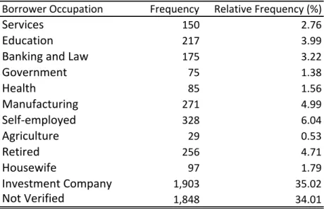
For those borrowers whose occupation is veri…ed, the di¤erent sectors of the economy

in which they are employed are described in Table 3: Self-employed borrowers are the single largest subgroup. Of those whose occupation is not veri…ed, approximately half are

investment companies. We will conduct all subsequent analysis separately for the veri…ed and non-veri…ed borrowers to allow for the possibility that the relaxation in the cosigner

requirement a¤ects the two groups di¤erently.

The defaults we measure re‡ect payments made by the borrower to the Rosca organizer –

and some of these may indeed be …nancial help that the borrower has received from cosigners –but not payments collected directly from the cosigners by the organizer. To understand

why this is so, it is useful to describe the long and costly collection process.7 When a borrower misses an installment, then the organizer sends a legal notice to the borrower

(after5months), another legal notice to borrower and cosigners (after6 months) and takes them to court (at 12 months if the amount is still overdue). The court begins to collect money from the cosigners approximately27months after the missed installment, and remits collection proceeds to the Rosca organizer around4years after the missed installment. The court also collects a12percent per year interest penalty on overdues. Our …eld interviews indicate that the Rosca organizer pushes through with this long costly collection process to

make its collateral threat credible.

Loan o¢ cers con…rmed that they never collect money directly from cosigners through

the long legal process, but only receive funds collected from cosigners through the court at the very end of the four-year process. Our measure of default is based on overdues

at the end of a Rosca. The earliest possible borrower (in February 2001) may indeed have missed repayments in March 2001, twenty-two months before the end of the Rosca.

7

Visaria (2006) …nds that legal reforms that improve loan collection in India have substantial e¤ects on repayment and interest rates.

But it is impossible for the organizer to have collected repayments from cosigners within those twenty-two months (since it takes at least four years). We are thus assured that our

default measure is based only on repayment by the borrower herself, not on money collected from the cosigners. This feature will allow us to distinguish whether cosigners promote

repayment or are simply an ex-post hedging device.

3

Empirical Strategy

Identification

Our empirical strategy is based on the rule of thumb that allows loan o¢ cers to relax the

cosigner requirement for borrowers in the middle of a Rosca. The identifying assumption is that loan terms such as the winning bid and the repayment burden change continuously

from round to round but the cosigner requirement changes discontinuously.

To illustrate, consider a 25 round Rosca in which the loan o¢ cer is allowed to ask for fewer cosigners in round13relative to round12: Our empirical approach will be to compare the default rates for round 13 borrowers with those of round 12 borrowers holding other loan terms constant. In other words, our test is whether round 13 loans are more likely to default compared with observationally identical round 12 loans. Our null hypothesis is that cosigners do not induce repayment by borrowers and so round13borrowers are just as likely to default as round12 borrowers holding other loan terms constant. Notice that the lender may indeed collect funds directly from cosigners through the legal process — and that possibility is consistent with our null hypothesis.

We should note one important issue of interpretation at the outset. Even if we …nd that relaxing the cosigner requirement reduces repayment in round 13 relative to round 12;we will not be able to distinguish why this might have occurred. In other words, an increase

in defaults could arise if the reduction in cosigners either (a) gave round 13 borrowers incentives to make riskier project choices or (b) gave riskier types the incentive to wait

cosigners to borrowers in round13relative to round12. Our null hypothesis is simply that cosigners are ine¤ective in simultaneously (a) preventing moral hazard, (b) screening bad

risks, and (c) providing insurance. So if we reject the null, we can conclude that cosigners are e¤ective in one or more of these three channels but cannot distinguish which one.

In this section, we …rst show why identi…cation is di¢ cult in the absence of exogenous variation in the cosigner requirement. We then discuss how the relaxation in the cosigner

requirement allows us to test if there is a causal relationship between the number of cosigners and defaults.

We start with some notation. In any Rosca loan, the debt incurred equals the sum of net repayments due from the Rosca winner who receives the pot at date t. Denote this

repayment burden byRt. Let the default rate, i.e. the fraction ofRtthat is unpaid at the end of the Rosca be denotedyt: Let btbe the winning bid at which the pot is obtained in

roundt. The winning bid is a measure of the price of capital.

In what follows we shall be careful about what dimensions of the borrower type are

(not) observed by the researcher and by the lender. We shall de…ne three measuresxt; zt and tof information about the riskiness of the roundtborrower that may/not be observed

by the lender or the researcher. The variablext represents publicly observed information. For instance, the lender and the researcher both observe the Rosca denomination and the

loan terms, bt and Rt; borrowers may reveal their riskiness by taking unattractive loan terms. The variablezt denotes the riskiness of the roundtborrower observed by the lender

and not by the researcher (i.e. the "soft information" described in the introduction). For instance, the lender may have local information on borrowers – or may have some sense

of their reliability by whether or not their previous contributions to the Rosca have been timely. Let t be the riskiness unobserved by both the lender and researcher, i.e. t

represents information that is truly private. For convenience, this information structure is summarized in the following table.

Observed by Lender Observed by Researcher

xt Yes Yes

zt Yes No

t No No

The lender’s choice of how many cosignersctto require of the borrower will depend on

all the information observed by the lender:

ct=c(t; Rt; bt; xt; zt) +vt; (1) where vt is a random error term with mean zero. For instance, the number of cosigners

required is likely to be nondecreasing in the debtRt, in the price that the borrower is willing to pay bt; and in the borrower’s riskiness zt: In general, a default yt will depend on the

loan terms, on the cosigners required and on the risk characteristics of the borrower both observed and unobserved by the lender:

yt=y(t; Rt; bt; ct; xt; zt; t) +ut; (2) whereE(utjt; Rt; bt; ct; xt; zt; t) = 0:

Our null hypothesis is that cosigners are ine¤ective at reducing defaults by the bor-rower. Since we measure defaults as payments collected from the borrower and not from

the cosigners, cosigners may be very useful as a source of funds for the lender, even when our null is true.

Consider the regression relating defaults and the cosigner requirement:

yt=Dy(t; y) + ct+a1Rt+a2bt+a3xt+ut; (3) where y is a vector of parameters,Dy is a (continuous) polynomial intcapturing the e¤ect of ton y. When we estimate (3) by OLS, the estimation su¤ers from an omitted variable problem: zt is not in the set of explanatory variables. So, under the null of ine¤ective

cosigning (which implies @_@c = 0), we would estimate > 0 if @c_@z > 0. In other words, cosigners are positively correlated with default rates because riskier borrowers are asked for

more cosigners than safer ones are and the riskinesszis unobserved by the researcher. The null hypothesis –that cosigners do not induce borrowers to repay –may be true despite the

positive estimate of :

Our approach to solve this problem is to exploit the discontinuity in the cosigner

assign-ment rule at the middle round (the institutional details were discussed in section 2): We maintain the assumption that the functions in (2) and (1) are continuous in all arguments.

Let the dummy variable latet denote rounds after the middle with the relaxed cosigner requirement, i.e. all roundst 13:We may then write the cosigner requirement as:

ct=c(t; Rt; bt; xt; zt; latet) +vt (4) Notice, moreover, that, conditional on ct,yt is not a function of latet as only the cosigner

rule changes discontinuously at the middle round.

We will test if there is a trend break in the cosigner requirement in the middle round

by estimating

ct=D(t; c) + latet+d1Rt+d2bt+d3xt+vt: (5) The OLS estimate of in (5) will capture the sum of two e¤ects: …rst the direct e¤ect of

latet on ct and, second, the indirect e¤ect of selection on zt:

b= c late+ @c @z z late (6)

A relaxation in the cosigner requirement would imply _latec < 0: If observably riskier borrowers wait until the cosigner relaxation to borrow, then _latez >0;and since the lender is likely to ask observably riskier borrowers for more cosigners, _@z@c >0; this indirect e¤ect will be positive. If the indirect e¤ect around the middle round is su¢ ciently strong, then

we may estimate = 0. In what follows, we show that for a certain subset of riskier borrowers, this is indeed what happens.

We will test if there is a corresponding trend break in defaults in the middle round by estimating:

yt=D(t; y) + late+a1Rt+a2bt+a3xt+ut; (7) The OLS estimate of in (7) will capture the sum of two e¤ects:

b= @y @c c late + @y @(z+ ) (z+ ) late (8)

Under the null hypothesis there are no moral hazard/insurance or selection e¤ects, i.e @y_@c = 0

and (z_late+ ) = 0. So the null is <0and = 0.

As deviations from our null hypothesis, we can think of several possibilities. If cosigners

reduced defaults by preventing moral hazard or by providing insurance, then @y_@c <0 and so the e¤ect of a relaxation in the cosigner requirement _latec < 0 would be to increase defaults in the middle round. If cosigners prevented defaults by attracting safer borrowers, then riskier borrowers would wait till after the middle round, (z_late+ ) >0;and since riskier borrowers are more likely to default _@(z@y_{+ )} >0;this would increase defaults in the middle round as well. In both cases then, we’d expectb>0:

Our empirical strategy may resemble regression discontinuity methods — but there is one important di¤erence. If the discontinuity in the number of cosigners was unanticipated,

then we would expect no selection on either or z around the middle round. Borrowers who took loans at similar terms just before and just after the median round would be "as

good as randomly assigned." We could then estimate the treatment e¤ect of cosigners on repayment (through preventing moral hazard or providing insurance) by using the latet

dummy as an instrument for the number of cosigners in regression (3). But in practice the relaxation in the cosigner requirement in the middle round is public information. We

therefore cannot rule out the possibility that riskier types will delay borrowing till just after the middle round. This form of selection may result in an upward trend break in defaults

– and arguably is an e¤ect of cosigners that we wish to capture.8 So we do not use the instrumental variable technique (or equivalently fuzzy regression discontinuity methods; see

8

In related research we …nd evidence that adverse selection is indeed a concern in these markets (Klonner and Rai, 2007).

Imbens and Lemieux, 2008) to isolate the treatment e¤ect of cosigners on defaults. Instead we shall interpret the coe¢ cient in regression (7) as the combined treatment and selection

e¤ect of cosigners on defaults provided <0:

One way in which loan o¢ cers may respond to the relaxation allowed in the number

of cosigners in the middle round of Roscas is by asking for each of the fewer cosigners to pledge more salary as collateral. As we mentioned in Section 2, the salary information on

cosigners was not available from the Rosca organizer – and so we have no way of directly testing whether there was such a substitution (from quantity to total salary of cosigners).

That said, asking for more salary per cosigner after the middle round and provided that a higher cosigner salary causes higher repayment by the borrower, our estimates of the causal

e¤ect in (7) would be biased downwards. So if anything, our estimated causal e¤ects are lower bounds.

Implementation

As we discussed in section 2 our sample consists of247Roscas of 25month durations with four di¤erent denominations. To implement speci…cation (3), which relates defaults to the cosigner requirement, we shall estimate the following:

ykit= kt+ ckit+a1Rkit+a2bkit+a3xkit+ukit (9) where ykit is the default measure for the borrower in round t of Rosca i of denomination

k; ckit is the cosigners required, Rkit is the repayment burden, bkit is the winning bid and

the controls xit are dummies for the 18 branch locations of the Rosca organize and 12 dummies for occupational categories (described in Table 3). These controls are included in all subsequent regressions as well.

Next, to investigate the causal link between cosigners and defaults in speci…cations (5)

and (7), we will estimate the following equation for the cosigners required,

ckit= S X

wheretdenotes the round andidenotes the Rosca group,kdenotes the Rosca denomination and S is the order of the polynomial. In other words, we allow for a di¤erent polynomial

function of degree S for each of the four denominations.

In our setting the treatment assignment depends on a discrete variable (the round in

which the loan was taken). Since the cosigner relaxation occurs in round 13 (compared with round 12), it is impossible to compare default rates for borrowers just above and just below the threshold round. If, in contrast, the treatment-determining variable was continuous, there would be observations arbitrarily close to the threshold available at least

as the sample size grows large. From those, the precise shape of the regression function around the threshold (and thus the discontinuity itself) could be estimated consistently by

nonparametric methods. In our discrete case, however, the discontinuity in default rates has to be estimated by assuming a parametric form for the regression function. Any particular

parametric form is only an approximation of the true regression function, however. Even as the number of observations becomes large, the regression function around the discontinuity

will be estimated with an error.

Lee and Card(2008)model these speci…cation errors as random and suggest a procedure to select the appropriate parametrization, i.e. the order of the polynomial in (10). We implement their procedure as follows. To determine the degree of the polynomial which is

appropriate, S, we conduct a likelihood ratio test of (10) against

ckit= kt+d1Rkit+d2bkit+d3xkit+ukit:

As we use rounds2to23of each Rosca, the resulting chi-square statistic has22 4 (4S+ 1) = 87 4S degrees of freedom. We then choose the smallest value ofS that fails to reject our likelihood ratio speci…cation test at the10 per cent level.

We use the same procedure to determine the order of the polynomial for the default equation,

ykit= S X s=0

ksts+ latet+a1Rkit+a2bkit+a3xkit+ukit: (11) Lee and Card (2008) also show that statistical inference will account for the

speci…ca-tion errors in parametrizaspeci…ca-tion by clustering the standard errors by the treatment assignment variable. We therefore cluster the standard errors obtained from (10) and (11) by t to

account for potential remaining speci…cation error of the polynomial vis-a-vis the unob-served, "true" form of D(t; ) in (5) and (7). Finally, we estimate all equations, including those with dichotomous or censored dependent variables, by OLS because the theory on regression discontinuity with speci…cation error does not readily extend to probit and tobit

models.

4

Results

In this section we present our main empirical …ndings. Loans that have a higher cosigner

requirement initially are more likely to go into default ex post. Despite this positive correlation between cosigners and defaults, however, there is a negative causal link. We

…nd that there is a reduction in cosigners in the middle round for those borrowers whose occupation is not veri…ed –and this reduction is associated with an increase in defaults for

those borrowers around the middle round.

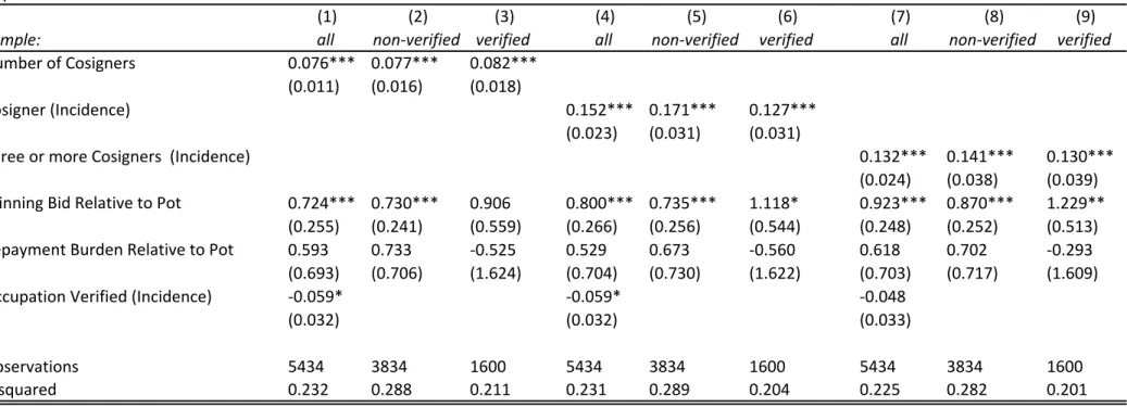
We …rst investigate the reduced-form relationship between the number of cosigners

at-tached to a loan and defaults based on speci…cation (9) in Tables 4and 5. The incidence of defaults is the dependent variable in Table 4; while the default rate is the dependent variable in Table 5: For all three measures of the cosigner requirement – and for both the occupation-veri…ed and the non-veri…ed subsamples – there is a strong and signi…cant

positive relationship between cosigners required and defaults. For instance, the point esti-mate of 0:076 in column 1 of Table 4 implies an increase in default probability of roughly one-eighth for each additional cosigner attached to the loan. Put di¤erently, doubling the number of cosigners will on average increase the incidence of defaults by 5 percent. An analogous pattern arises when default rate is the dependent variable (Table5). The magni-tude of this positive correlation between defaults and cosigners does not di¤er signi…cantly

across subgroups in our sample.

middle round causes a discontinuous increase in defaults in the middle round. Recall from section 3 that we expect a trend break in the cosigner requirement, <0 in speci…cation (10), if there is a reduction in the number of cosigners as speci…ed by the Rosca guidelines –and an increase in defaults, >0 in speci…cation (11), as a consequence.

Is there a trend break in cosigners required? The OLS estimates in Table 6 are based on speci…cation (10) for the pooled sample and for the occupation-veri…ed and non-veri…ed

subsamples for each of the three cosigner measures. The estimated coe¢ cient onlateit is negative and signi…cant for those borrowers who are perceived to be safer (occupation not

veri…ed). The trend break in the cosigner requirement for the non-veri…ed subsample is substantial: the point estimate of 0:163in column2, for instance, is more than a third of the average number of cosigners for this subsample (0:426from Table2): Similar orders of magnitude de…ne the downward trend break for the incidence of one or more cosigners and

for the incidence of three or more cosigners around the middle round for this subsample.9 There is no signi…cant e¤ect for the riskier borrowers (occupation veri…ed) nor for the pooled

sample. Recall from section 3, that we might expect the lender not to relax the cosigner requirement for riskier borrowers to prevent them from waiting to take loans in round 13:

Table 6 also reveals other determinants of the cosigner requirement. Occupation-veri…ed borrowers are asked to pledge roughly a third more cosigners than the average borrower

(column 1): Higher winning bids are associated with higher cosigner requirements: a ten percentage point increase in the winning bid results in 0:36 more cosigners required on average (column 1). The winning bid appears to be a much stronger signal to the lender

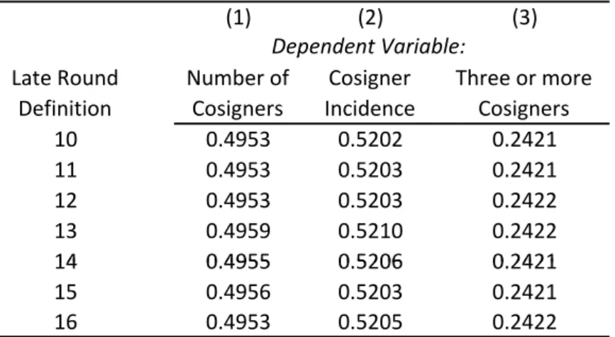
9_{To check whether the thirteenth round of a Rosca is the appropriate break point, we also estimate}

equation (10) for the subsample of non-veri…ed borrowers with alternative speci…cations of thelate-dummy. In particular, we use alternative breaks occuring in the 10th, 11th, 12th, 14th, 15th and 16th round, respec-tively, and calculate the resultingR2_{-statistics. In each of these speci…cations, we use the same polynomial} orders as in columns 2, 5 and 8 of Table 6. The results are in Table A1. For the number of cosigners and the cosigner incidence, theR2-statistic is maximized for a trend break in round 13 and for our third cosigner measure, the 13th round break is still a weak maximizer of the R2_{-criterion. We take this as empirical} support for our identifying assumption that loan o¢ cers apply the the company’s published cosigner rule in the form of a trend break at the middle round (round13)of a Rosca.

for borrowers who are deemed riskier (the point estimate of the coe¢ cient on winning bids in column3 is more than twice the point estimate in column 2).

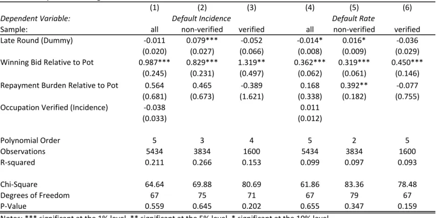
Is there a trend break in defaults? The OLS estimates in Table 7 are based on speci-…cation (11). There is a signi…cant upward jump in default incidence for the non-veri…ed

borrowers but not for the occupation-veri…ed borrowers. Put di¤erently, the estimated coe¢ cient onlateit is negative and signi…cant for those borrowers who are perceived to be

safer and the e¤ect is large: the point estimate of0:079is one eighth of the average default incidence for nonveri…ed borrowers. Tables 6 and 7together show that a reduction in the number of cosigners of a little less than a third results in an increase in the incidence of default of a little more than ten percent. This is a substantial causal e¤ect of cosigners

on defaults of borrowers perceived to be safer. (We cannot of course tell what the e¤ect of cosigners was on those borrowers whose occupation was veri…ed because they were

per-ceived to be riskier.) The results using the default rate measure are less conclusive possibly because there is less variation in this measure relative to default incidence.

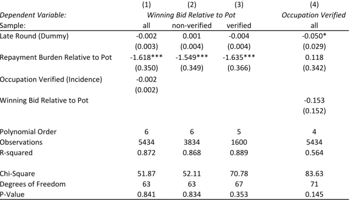
In Table 8 we ask if there is a discontinuous change in the winning bids around the middle round. If cosigners are costly (in terms of their monitoring or selectivity), then

riskier borrowers may be willing to pay a premium in round 13 for a relaxation in the cosigner requirement – implying a upward trend break in winning bids around the middle

round. On the other hand, those una¤ected by the cosigner relaxation would have an incentive arbitrage away any discontinuous di¤erences in winning bids. Occupation-veri…ed

borrowers who have little incentive to wait till round13 would bid up the price of a loan in round12. The estimates in columns1 3of Table 8are suggestive of the latter story.

We also …nd in column4that there is a relaxation in occupation (and income) veri…cation after the middle round. This is consistent with our earlier evidence (Table 6)that such borrowers perceived by the loan o¢ cer to be riskier do not enjoy a relaxation in the cosigner requirement –and hence have little incentive to wait till round13. Borrowers perceived to be safer would rather wait for the cosigner relaxation in round13than take loans in round

the lender’s perceived riskiness of borrowers. In sum, it is consistent to observe both a discontinuous decrease in riskiness (and hence occupation veri…cation) but no discontinuous

change in the winning bids.

Finally, note that the polynomial order for each regression reported in Tables6;7and 8

are determined by the likelihood ratio test described in Section 3, and standard errors are clustered by round.

5

Conclusion

In this paper we investigate the use of cosigners as collateral using data from South India. We show that the number of cosigners is positively correlated with defaults – presumably

because borrowers who are high default risks are asked for more cosigners. This is very similar to the positive correlation …nding in the empirical collateral literature. We go further

to investigate whether there is a causal link between the number of cosigners required on a loan and the subsequent default probability. We use a rule-of-thumb relaxation in the

number of cosigners required on shorter duration loans to isolate this causal e¤ect. This relaxation is orthogonal to any soft information about the borrower privately observed by

the loan o¢ cer –and hence allows us to isolate the e¤ect of reducing the number of cosigners on defaults.

Our …ndings are broadly consistent with models in which ex-ante riskier borrowers are asked for more cosigners and cosigners reduce defaults ex-post. One such model that has

both the positive correlation and the negative causation between collateral and defaults is by Boot, Thakor and Udell (1991). In their model the collateral is provided by borrowers

– but the same results would apply if collateral were provided by cosigners instead. Bor-rowers di¤er in terms of observed riskiness and are subject to moral hazard. Lenders ask

observably riskier borrowers for more collateral (positive correlation) – yet collateral also has an incentive e¤ect (negative causal e¤ect). Simpler models which just have a positive

correlation between cosigners and defaults but no causal link – or a negative causal link but no correlation – are not consistent with what we …nd. Models in which cosigners are

merely a source of funds for the lender ex-post are also inconsistent with our results. Finally, our paper points to the usefulness of cosigners –but we cannot with the available

data distinguish between the channels through which cosigners operate. In other words, do cosigners select safer types of borrowers – or induce safer project choices – or do they

insure borrowers against bad luck? We leave these interesting issues for future research.

References

[1] Ahlin, C. and R. Townsend, 2007: Using repayment data to test across models of joint liability lending. Economic Journal, 117: F11-51

[2] Baker, A. B.,1977. Community and Growth: Muddling Through with Russian Credit Cooperatives. Journal of Economic History 37, 139-160.

[3] Banerjee, A., T. Besley and T. Guinnane, 1994. Thy Neighbor’s Keeper: The Design of a Credit Cooperative with Theory and a Test. Quarterly Journal of Economics 109, 491-515.

[4] Banerjee, A. 2003: “Contracting Constraints, Credit Markets and Economic Devel-opment”in Dewatripont, M., L. Hansen and S. Turnovsky eds. Advances in Economic Theory and Econometrics: Theory and Applications, Theory and Applications, Eight

World Congress of the Econometric Society, Cambridge University Press, 1-46.

[5] Berger, A.N. and G.F. Udell, 1990. Collateral, loan quality, and bank risk. Journal of Monetary Economics 25, 21–42.

[6] Berger, A. N. and G. Udell, 1998. The Economics of Small Business Finance: The

Roles of Private Equity and Debt Markets in the Financial Growth Cycle, Journal of Banking and Finance 22, 613-673.

[7] Besley, T., S. Coate and G. Loury,1993:The Economics of Rotating Savings and Credit Associations. American Economic Review 83, 792-810.

[8] Besanko, D. and A.V. Thakor, 1987. Collateral and rationing: sorting equilibria in monopolistic and competitive credit markets. International Economic Review 28, 671–

689.

[9] Bond, P. and A.S. Rai, 2008: Cosigned or Group Loans. Journal of Development Economics. 85: 58-80.

[10] Boot, A.W.A., Thakor, A.V., Udell, G.F., 1991. Secured lending and default risk:

equilibrium analysis, policy implications and empirical results. Economic Journal 101, 458–472.

[11] Gine, X. and D. Karlan,2008: Peer Monitoring and Enforcement: Long Term Evidence from Microcredit Lending Groups with and without Group Liability. Working Paper.

[12] Guinnane, T. W.,1994:A Failed Institutional Transplant: Rai¤eisen’s Credit Cooper-atives in Ireland, 1894-1914, Explorations in Economic History 31:1, 38-61.

[13] Imbens, G.W. and T. Lemieux, 2008: Regression Discontinuity Designs: A Guide to Practice. Journal of Econometrics 142: 615-635.

[14] Jiménez, G.,V. Salas and J. Saurina, 2006: Determinants of collateral, Journal of Fi-nancial Economics 81: 255–281.

[15] Karlan, D. 2007: Social Connections and Group Banking Economic Journal, 117: F52-F84

[16] Klonner, S., A.S. Rai 2007: Adverse Selection in Credit Markets: Evidence from a Policy Experiment. Working Paper.

[17] Lee, D.S. and D. Card, 2008: Regression Discontinuity Inference with Speci…cation Error. Journal of Econometrics 142: 655-674.

[18] Newton, L.,2000. Trust and Virtue in Banking: the Assessment of Borrowers by Bank Managements at the Turn of the Twentieth Century. Financial History Review 7, 177-199.

[19] Phillips, R.J. and D. Mushinski,2001. The Role of Morris Plan Lending Institutions in Expanding Consumer Micro-Credit in The United States. Working Paper, Department

of Economics, Colorado State University.

[20] Petersen, M. and R.G. Rajan, 1994. The bene…ts of lending relationships, Journal of Finance 49, 3–37.

[21] Pozzolo, Z., 2004. The Role of Guarantees in Bank Lending. Discussion Paper No. 528,

Banca D’Italia.

[22] Rai, A. and T. Sjöström, 2004. Is Grameen Lending E¢ cient? Repayment Incentives and Insurance in Village Economies. Review of Economic Studies 71, 217-234.

[23] Townsend, R.1997: “Microenterprise and Macropolicy”in Kreps, D. and K. Wallis eds. Advances in Economics and Econometrics: Theory and Applications, Seventh World Congress of the Econometric Society, Cambridge University Press, II:160-209.

[24] Uzzi, B. and R. Lancaster, 2003. Relational embeddedness and learning: The case of bank loan managers and their clients. Management Science 49, 383-399.

[25] Visaria, S. 2006: Legal Reform and Loan Repayment: The Microeconomic Impact of Debt Recovery Tribunals in India. Working Paper, Boston University.

[26] Vaidyanathan, R. and K. Sriram, 2000. The Non-Banking Financial Sector. Indian Institute of Management, Bangalore. mimeo.

[27] Wydick, B. 1999. Can Social Cohesion Be Harnessed to Repair Market Failures? Evi-dence from Group Lending in Guatemala. Economic Journal, 109: 2015–75.

Table 1. Rosca Characteristics

Contribution (Rs.) Pot Value (Rs.) Number of Groups

Percentage in  Sample 400 10,000 94 38.06 1,000 25,000 65 26.32 2,000 50,000 62 25.10 4,000 100,000 26 10.53

Table 2. Descriptive Statistics

Sample: All Occupation not verified Occupation verified

Mean Std. Dev. Min Max Mean Std. Dev. Min Max Mean Std. Dev. Min Max Winning Bid Relative to Pot 0.162 0.092 0.050 0.300 0.158 0.089 0.050 0.300 0.171 0.097 0.050 0.300 Repayment Burden Relative to Pot 0.467 0.225 0.074 0.885 0.465 0.230 0.077 0.885 0.472 0.215 0.074 0.860

Late Round (Incidence) 0.500 0.500 0 1 0.504 0.500 0 1 0.491 0.500 0 1

Borrower Occupation Verified by Lender (Incidence) 0.294 0.456 0 1 0.000 0.000 0 0 1.000 0.000 1 1

Number of Cosigners 0.717 1.057 0 6 0.426 0.873 0 5 1.414 1.132 0 6

Cosigner (Incidence) 0.380 0.485 0 1 0.233 0.423 0 1 0.730 0.444 0 1

Three or more Cosigners  (Incidence) 0.105 0.306 0 1 0.057 0.232 0 1 0.219 0.414 0 1

Default (Incidence) 0.614 0.487 0 1 0.606 0.489 0 1 0.633 0.482 0 1

Default Rate 0.103 0.152 0 1 0.090 0.141 0 1 0.133 0.173 0 1

Observations 5434 3834 1600

Notes: Repayment Burden is the sum of net contributions (required contributions less dividends) due from a Rosca winner in round t in rounds  t+1, t+2...T, where T is the last month of the Rosca. Default rate refers to amount outstanding relative to liability at the termination of the Rosca.

Table 3. Occupational Characteristics of Borrowers

Borrower Occupation Frequency Relative Frequency (%)

Services

Education

Banking

and

Law

Government

Health

Manufacturing

Self

‐

employed

Agriculture

Retired

Housewife

Investment

Company

Not

Verified

Table 4. Regression Analysis of Default Incidence Dependent Variable: Default Incidence

(1) (2) (3) (4) (5) (6) (7) (8) (9)

Sample: all non‐verified verified all non‐verified verified all non‐verified verified

Number of Cosigners 0.076*** 0.077*** 0.082*** (0.011) (0.016) (0.018)

Cosigner (Incidence) 0.152*** 0.171*** 0.127***

(0.023) (0.031) (0.031)

Three or more Cosigners  (Incidence) 0.132*** 0.141*** 0.130***

(0.024) (0.038) (0.039) Winning Bid Relative to Pot 0.724*** 0.730*** 0.906 0.800*** 0.735*** 1.118* 0.923*** 0.870*** 1.229**

(0.255) (0.241) (0.559) (0.266) (0.256) (0.544) (0.248) (0.252) (0.513)

Repayment Burden Relative to Pot 0.593 0.733 ‐0.525 0.529 0.673 ‐0.560 0.618 0.702 ‐0.293

(0.693) (0.706) (1.624) (0.704) (0.730) (1.622) (0.703) (0.717) (1.609)

Occupation Verified (Incidence) ‐0.059* ‐0.059* ‐0.048

(0.032) (0.032) (0.033)

Observations 5434 3834 1600 5434 3834 1600 5434 3834 1600

R‐squared 0.232 0.288 0.211 0.231 0.289 0.204 0.225 0.282 0.201

Standard errors in parentheses.

All specifications include dummies for 22 Rosca rounds, 12 occupation categories, 4 Rosca denominations, and 18 branch locations. Notes: *** significant at the 1% level, ** significant at the 5% level, * significant at the 10% level

Table 5. Regression Analysis of Default Rate Dependent Variable: Default Rate

(1) (2) (3) (4) (5) (6) (7) (8) (9)

Sample: all non‐verified verified all non‐verified verified all non‐verified verified

Number of Cosigners 0.030*** 0.031*** 0.036*** (0.005) (0.007) (0.008)

Cosigner (Incidence) 0.053*** 0.057*** 0.051***

(0.011) (0.015) (0.014)

Three or more Cosigners  (Incidence) 0.060*** 0.069*** 0.066***

(0.011) (0.016) (0.014) Winning Bid Relative to Pot 0.259*** 0.292*** 0.277 0.299*** 0.307*** 0.377** 0.334*** 0.345*** 0.412**

(0.062) (0.063) (0.170) (0.063) (0.066) (0.164) (0.063) (0.067) (0.152)

Repayment Burden Relative to Pot 0.178 0.389 ‐0.167 0.155 0.363 ‐0.174 0.191 0.382 ‐0.064

(0.340) (0.243) (0.741) (0.349) (0.245) (0.784) (0.335) (0.241) (0.751)

Occupation Verified (Incidence) 0.003 0.004 0.007

(0.011) (0.011) (0.012)

Observations 5434 3834 1600 5434 3834 1600 5434 3834 1600

R‐squared 0.128 0.134 0.160 0.122 0.130 0.147 0.119 0.125 0.149

Notes: *** significant at the 1% level, ** significant at the 5% level, * significant at the 10% level. Standard errors in parentheses.

Table 6. Analysis of the Lender's Cosigner Rule

(1) (2) (3) (4) (5) (6) (7) (8) (9)

Dependent Variable: Number of Cosigners Cosigner Incidence Three or more Cosigners (Incidence)

Sample: all non‐verified verified all non‐verified verified all non‐verified verified

Late Round (Dummy) ‐0.105 ‐0.163*** ‐0.129 ‐0.058* ‐0.062*** ‐0.057 0.003 ‐0.027** 0.039

(0.065) (0.052) (0.140) (0.030) (0.017) (0.069) (0.022) (0.010) (0.048)

Winning Bid Relative to Pot 3.632*** 2.434*** 5.064*** 1.336*** 1.068*** 1.713*** 0.601*** 0.347** 0.731***

(0.385) (0.398) (0.483) (0.197) (0.190) (0.301) (0.138) (0.132) (0.176)

Repayment Burden Relative to Pot ‐0.247 ‐1.199 3.076 0.337 ‐0.163 1.997*** ‐0.310 ‐0.447 ‐0.134

(0.835) (0.930) (1.912) (0.323) (0.305) (0.597) (0.313) (0.358) (0.740)

Occupation Verified (Incidence) 0.228*** 0.115*** 0.046***

(0.034) (0.017) (0.016) Polynomial Order 4 8 4 4 5 4 10 9 13 Observations 5434 3834 1600 5434 3834 1600 5434 3834 1600 R‐squared 0.569 0.496 0.549 0.554 0.521 0.297 0.331 0.242 0.457 Chi‐Square 68.81 68.14 85.05 81.76 78.64 77.80 59.07 53.74 38.27 Degrees of Freedom 71 55 71 71 67 71 47 51 35 P‐Value 0.164 0.110 0.122 0.180 0.156 0.271 0.111 0.370 0.323

Standard errors, clustered by Rosca round, in parentheses.

All specifications include dummies for 12 occupation categories, 4 Rosca denominations, and 18 branch locations. Notes: *** significant at the 1% level, ** significant at the 5% level, * significant at the 10% level

Table 7.  Analysis of the Cosigner Rule and Defaults.

(1) (2) (3) (4) (5) (6)

Dependent Variable: Default Incidence Default Rate

Sample: all non‐verified verified all non‐verified verified

Late Round (Dummy) ‐0.011 0.079*** ‐0.052 ‐0.014* 0.016* ‐0.036

(0.020) (0.027) (0.066) (0.008) (0.009) (0.029)

Winning Bid Relative to Pot 0.987*** 0.829*** 1.319** 0.362*** 0.319*** 0.450***

(0.245) (0.231) (0.497) (0.062) (0.061) (0.146)

Repayment Burden Relative to Pot 0.564 0.465 ‐0.389 0.168 0.392** ‐0.077

(0.681) (0.673) (1.621) (0.338) (0.182) (0.755)

Occupation Verified (Incidence) ‐0.038 0.011

(0.033) (0.012) Polynomial Order 5 3 4 5 2 5 Observations 5434 3834 1600 5434 3834 1600 R‐squared 0.211 0.266 0.153 0.099 0.097 0.093 Chi‐Square 64.64 69.88 80.69 61.86 83.36 78.48 Degrees of Freedom 67 75 71 67 79 67 P‐Value 0.559 0.645 0.202 0.655 0.347 0.159

Standard errors, clustered by Rosca round, in parentheses.

All specifications include dummies for 12 occupation categories, 4 Rosca denominations, and 18 branch locations. Notes: *** significant at the 1% level, ** significant at the 5% level, * significant at the 10% level

Table 8.  Cosigner Rule, Winning Bids and Borrower Screening.

(1) (2) (3) (4)

Dependent Variable: Winning Bid Relative to Pot Occupation Verified

Sample: all non‐verified verified all

Late Round (Dummy) ‐0.002 0.001 ‐0.004 ‐0.050*

(0.003) (0.004) (0.004) (0.029)

Repayment Burden Relative to Pot ‐1.618*** ‐1.549*** ‐1.635*** 0.118

(0.350) (0.349) (0.366) (0.342)

Occupation Verified (Incidence) ‐0.002 (0.002)

Winning Bid Relative to Pot ‐0.153

(0.152) Polynomial Order 6 6 5 4 Observations 5434 3834 1600 5434 R‐squared 0.872 0.868 0.889 0.564 Chi‐Square 51.87 52.11 70.78 83.63 Degrees of Freedom 63 63 67 71 P‐Value 0.841 0.834 0.353 0.145

Standard errors, clustered by Rosca round, in parentheses.

All specifications include dummies for 12 occupation categories, 4 Rosca denominations, and 18 branch locations. Notes: *** significant at the 1% level, ** significant at the 5% level, * significant at the 10% level

Table A1. Goodness of Fit of Alternative Late Round Definitions (1) (2) (3) Dependent Variable:p Late Round  Definition Number of  Cosigners Cosigner  Incidence Three or more  Cosigners 10 0.4953 0.5202 0.2421 11 0.4953 0.5203 0.2421 12 0.4953 0.5203 0.2422 13 0.4959 0.5210 0.2422 14 0 4955 0 5206 0 2421 14 0.4955 0.5206 0.2421 15 0.4956 0.5203 0.2421 16 0.4953 0.5205 0.2422

Notes: each cell displays the R‐Squared statistic from a regression 

with only non‐verified borrowers. In each regression

the Late Round dummy is equal to zero for rounds earlier than the value in the "Late Round Definition" column, and equal to one otherwise. Columns 1, 2 and 3 of this table correspond to columns 2, 5 and 8 of Table 6, respectively.