This is a peer-reviewed, post-print (final draft post-refereeing) version of the following published document:
Olper, A. and Raimondi, V. and Cavicchioli, D. and Vigani, Mauro (2014) Do CAP payments reduce farm labour migration? A panel data analysis
across EU regions. European Review of Agricultural Economics, 41 (5). pp. 843-873. ISSN 0165-1587
Official URL: http://dx.doi.org/10.1093/erae/jbu002 DOI: http://dx.doi.org/10.1093/erae/jbu002
EPrint URI: http://eprints.glos.ac.uk/id/eprint/2886 Disclaimer
The University of Gloucestershire has obtained warranties from all depositors as to their title in the material deposited and as to their right to deposit such material.
The University of Gloucestershire makes no representation or warranties of commercial utility, title, or fitness for a particular purpose or any other warranty, express or implied in respect of any material deposited. The University of Gloucestershire makes no representation that the use of the materials will not infringe any patent, copyright, trademark or other property or proprietary rights.
The University of Gloucestershire accepts no liability for any infringement of intellectual property rights in any material deposited but will remove such material from public view pending investigation in the event of an allegation of any such infringement.
This is a peer-reviewed, post-print (final draft post-refereeing) version of the following published document:
Olper, A. and Raimondi, V. and Cavicchioli,
D. and Vigani, Mauro (2014).
Do CAP payments
reduce farm labour migration? A panel data analysis
across EU regions.
European Review of Agricultural
Economics, 41 (5), 843-873. ISSN 0165-1587
Published in European Review of Agricultural Economics, and available online at:
http://erae.oxfordjournals.org/content/41/5/843
We recommend you cite the published (post-print) version.
The URL for the published version is http://dx.doi.org/10.1093/erae/jbu002
Disclaimer
The University of Gloucestershire has obtained warranties from all depositors as to their title in the material deposited and as to their right to deposit such material.
The University of Gloucestershire makes no representation or warranties of commercial utility, title, or fitness for a particular purpose or any other warranty, express or implied in respect of any material deposited.
The University of Gloucestershire makes no representation that the use of the materials will not infringe any patent, copyright, trademark or other property or proprietary rights.
The University of Gloucestershire accepts no liability for any infringement of intellectual property rights in any material deposited but will remove such material from public view pending investigation in the event of an allegation of any such infringement.
1
Do CAP Payments Reduce Farm Labour Migration?
A Panel Data Analysis Across EU Regions
Version: October 2013 Abstract
This paper deals with the determinants of out-farm migration across the EU regions focusing on the role played by CAP payments. We add to the existing literature in three main directions. First, our analysis has broad coverage (150 EU regions over the 1990-2009 period); second, we work on the entire portfolio of CAP instruments; third, we rely on modern panel data methods. Results show that standard drivers, like the relative income and the relative labour share, are important determinants of out-farm migration. Overall, CAP payments significantly contributed to maintain job in agriculture, though the magnitude of the economic effect has been quite moderate and heterogeneous across policy instruments. Pillar I subsidies exerted an effect more than two times greater than that of Pillar II payments. JEL codes: Q12, Q18, O13, J21, J43, J60.
Keywords: Out-farm Migration, Labour Markets, CAP Payments, Panel Data Analysis.
1. Introduction
Over the last fifty years European Union (EU) countries have experienced important adjustments in the agricultural labour market, showing an impressive out-farm migration of the labour force.1 Although in the last decades we assisted to a certain slowdown of the rate of out-farm migration, it remains positive in almost all the Regions of the EU-15 countries (see Figure 1). These stylized facts are at odds with more than €50 billion of income subsidies per year spent by the Common Agricultural Policy (CAP).
1 In this paper, by the term “out-farm migration” we mean labour exit from agriculture, irrespective of whether
this process happens through a simple exit from the sector, or a genuine process of labour reallocation from agriculture to non-agriculture sector.
2 The creation and maintenance of jobs in agriculture and in rural areas has been a traditional CAP target, an objective recently restated and emphasized by several EU official documents (e.g. European Commission, 2010; European Parliament, 2010).2 However, the effectiveness of subsidies in maintaining the labour force into the agricultural sector is actually unclear and the empirical evidence is still largely inconclusive. In the literature there are papers that find a negative impact of subsidies on out-farm migration (e.g. Breustedt and Glauben, 2007; D’Antoni and Mishra, 2010), others that find no effect (e.g. Barkley, 1990; Glauben et al. 2006; Petrick and Zier, 2012), and even papers that find a positive effect of subsidies on out-farm migration (e.g. Dewbre and Mishra, 2007; Petrick and Zier, 2011).
One possible reason for these counterintuitive effects is that agricultural subsidies are quite ineffective as income support policy, especially because of the imperfections in both input and output markets.3 In fact, many indirect channels have been emphasized through which farm subsidies may affect agricultural employment. For example, Barkley (1990) stressed that an indirect impact of subsidies may have occurred through increased land values.4 Indeed, land value appreciation slows down the rate of labour migration out of agriculture. Differently, Goetz and Debertin (1996) showed that capital-labour substitution effects, induced by farm subsidies, in the long-run may translate in a reduction of labour utilization. This effect may account for the positive relation between farm subsidies and out-farm migration. More recently, Berlinschi et al. (2011) found evidence of another indirect channel, the effect of subsidies on the educational level of farmers’ children and the resulting impact on long-term labour supply.
These and other indirect effects of farm subsidies clearly deserve attention to better understand the key mechanisms responsible for the puzzling outcomes on agricultural
2 The European Commission reflection about the future of the CAP “The CAP Toward 2020” (EC,
COM(2010) 672) explicitly addressed agricultural and rural labour issues in several sections of the document. Labour and rural area employment issues are also well represented in the recent European Parliament document on CAP reforms “On the Future of the CAP after 2013” (EP 439.972).
3 For example, an important OECD (2001) study emphasized that only 20% of all agricultural support policies
resulted in net farm income growth in the OECD countries, the bulk of the aid being dissipated to others, like the owners of production factors.
4 From this perspective, studies from the US often showed that landowners capture a substantial share of
subsidies (e.g. Goodwin et al., 2005; Kirwan, 2009; Lence and Mishra, 2003). However, the evidence from the EU is mixed, with recent papers showing that decoupled subsidies are only marginally capitalized into land values (Ciaian et al. 2011; Michalek et al. 2011; Ciaian and Kancs, 2012).
3 labour. However, in this paper we argue that when the direct effects of farm subsidies are properly and consistently estimated, at least in the context of the EU regions investigated here, on average, the farm support programs have had a negative effect on the out-farm migration. Thus, CAP subsidies have made their contribution to maintain job in agriculture. The empirical literature on the effects of agricultural subsidies on farm labour reflects two main different theoretical approaches.5 The first looks at agricultural household models to analyze the impact of subsidies on the allocation of household labour (Lee, 1965; Becker, 1965). In these models farm income support may affect farmers’ labour allocation decisions in a number of ways: increasing the marginal value of farm labour; increasing household wealth; reducing income variability. The second approach focuses on the entry and exit processes from one sector to another, using models of occupational choice that have their roots in the Todaro (1969) and Harris and Todaro (1970) two-sector model.
Within this class of models farm subsidies affect farmers’ labour allocation decisions
mainly through their effect on farm income relative to non-farm income activities.
These two different theoretical approaches are reflected in empirical works that can be roughly divided in two categories, studies at farm-household level based on farm-level data, and studies on the farm labour (re)allocation at aggregate (country or regional) level. In the first group, the use of micro-data allows to address the individual adjustment behavior in response to changes in factors affecting the household utility, such as different revenues sources. Within this stream of literature we can find papers based on cross-section analysis (Mishra and Goodwin, 1997; El-Osta et al., 2004), panel data studies (e.g. Pietola
et al., 2003; Gullstrand and Tezic, 2008) and, more recently, semi-parametric approaches (e.g. Pufahl and Weiss, 2009; Esposti, 2011a).6 Although farm-household studies present
5 A branch of literature also used computable general equilibrium (CGE) models to analyze the effects of the
CAP, and a small part of this literature provides estimates of direct and indirect effects of the CAP on agricultural employment. The majority of this works analyze specific rural-urban areas, for example, Greece in Psaltopoulos et al. (2006); Scotland and Greece in Balamou et al. (2008); and Czech Republic and Greece in Psaltopoulos et al. (2011). See, Shutes (2012) for an application to the EU27 labour markets.
6 Recently, there has been an increasing tendency to use semi-parametric methods (e.g. Pufahl and Weiss,
2009; Esposti, 2011a; Salvioni and Sciulli, 2011; Ciaian et al. 2011). These quasi-experimental methods have several advantages, but they also have drawbacks. For example, when applied to the Pillar I subsidies a quasi-horizontal measure finding suitable counterfactuals (controls) tends to be a challenge (see Esposti 2011a; 2011b). Moreover, the implicit assumption is that the treatment affects only farms been treated, disregarding the possibility that the policy exerts an indirect effect trough adjustments in factors markets (see Pufahl and Weiss, 2009).
4 several advantages, especially due to the richness of micro-data information, they also have limitations. First, it is not always clear to what extent such results, mostly based on survey data, are representative of the entire population. Second, and perhaps more importantly for our purpose, the impact of macroeconomic and geographical conditions, as well as of agricultural policies, cannot be analyzed in greater detail because such factors are usually constant across all farmers in a specific region, and the time dimension of these studies is typically very short (see Glauben et al. 2006).
The analysis at the aggregate level is, in principle, less data constrained, enhanced by panel data methods and providing results with broader coverage. The process of labour migration from one sector to another is assessed by controlling for structural variables such as country or regional relative income, unemployment, population densities, and institutional and policy variables. The econometric approaches for the aggregate studies range from cross-sectional (Breustedt and Glauben, 2007; Hennessy and Rehman, 2008), to time-series analyses (Barkley, 1990; D’Antoni and Mishra, 2010) and to panel data methods (Mundlak, 1979; Larson and Mundlak 1997; Petrick and Zier, 2011; 2012).7
Analysis concerning the EU have mainly investigated the effects of national public support policies, others than CAP payments, on out-farm migration at the single-country level (e.g. Pietola et al., 2003; Goodwin and Holt, 2002; Benjamin and Kimhi, 2006; Glauben et al., 2006), while only a few studies investigated the effects of the CAP subsidies. For both household and aggregate level empirical studies, actual evidence other than inconclusive in term of the direction of the policy effect, is often confined to specific countries or regions (Pufahl and Weiss, 2009; Hennessy and Rehman, 2008; Gullstrand and Tezic, 2008), mainly as a consequence of data limitation at the EU regional level. Most of the authors used a cross-sectional approach (Breustedt and Glauben, 2007; Hennessy and Rehman, 2008; Van Herck, 2009), while panel data analysis concerned only single countries and/or specific policies, such as Objective 1 or agri-environmental measures (Gullstrand and Tezic, 2008; Pufahl and Weiss, 2009; Salvioni and Sciulli, 2011). Within
7 At the macro level, so far no studies have investigated the labour effect of farm subsidies using
semi-parametric methods. In this regard, a potential promising method is that used by Becker et al. (2010), who applied a regression-discontinuity design, exploiting the discrete jump in the probability of EU transfer receipt at 75% threshold, for the identification of the causal effects of Objective 1 treatment on growth and employment.
5 this literature, the works of Petrick and Zier (2011 and 2012) represent two relevant exceptions. They used difference-in-difference and dynamic panel models, respectively, and exploit the entire portfolio of CAP payments showing from weak positive to no employment effects of CAP subsidies. However, their results focused on just three East German regions, are hardly extendable to the EU as a whole.
To sum up, actual evidence concerning the effect of CAP payments on out-farm migration is not only quite inconclusive but it also suffers several drawbacks. First, the evidence comes mostly from cross-sectional inference. Second, it is often focused on country or regional case studies whose findings are difficult to generalize to other countries and regions with wide differences in development, labour market institutions and farming structures. Third, it rarely takes into account the entire portfolio of CAP payments. Last, but not least, no particular effort has been done to account for potential problems of endogeneity bias of CAP payments.
The main objective of this paper is to offer a contribution that moves in that direction. Specifically, the paper investigates the effect of CAP payments on inter-sectoral labour reallocation, extending earlier studies in three main directions. First, our analysis has broad coverage, considering 150 EU regions over the period from 1990 to 2009. Second, the effects of CAP instruments are analyzed focusing on both Pillar I payments (coupled and decoupled subsidies) and on several Pillar II rural development measures. Third, we rely on modern panel data methods, estimating both static and dynamic out-farm migration equations in order to account for several identification issues like unobserved heterogeneity, dynamics and endogeneity. Finally, we deliver a back-of-the-envelope calculation of the net benefits of the CAP in terms of job maintenance in agriculture.8
The remainder of the paper is organized as follows. Section 2 summarizes the conceptual framework from which we motivate the empirical strategy to investigate the effect of CAP subsidies on agricultural labour, developed in Section 3. Section 4 describes the data and how we measure the CAP payments at the EU regional level. Section 5 presents and discusses the results and, finally, Section 6 concludes.
8 For a recent interesting contribution that measured job creation and job destruction in the EU agriculture,
6
2. Conceptual framework and hypotheses
The paper is empirical in nature. However, to motivate our work we rely on the theory of occupational choice and labour migration decision, which has its roots in the Todaro (1969) and Harris and Todaro (1970) two-sectors model, subsequently developed further by Mundlak (1978) and Barkley (1990).
2.1 Out-farm migration equation
Consider a two sectors economy – agriculture (a) and non-agriculture (n) – where there is no room for uncertainty, capital market restrictions, and adjustment costs (see Breustedt and Glauben, 2007). Individuals choose between working in the agricultural or in the non-agricultural sector, by comparing their expected discounted lifetime utility in the two sectors, with consumption equal to income. The utility derived from one occupation, � , � , , is a function of the expected income (Y), the time spent working (L), plus exogenous shifters (Z), with �� �⁄ > .
Migration from one sector to the other will occur when the labour market is in disequilibrium, namely when there are differences between the return to labour in the two sectors. When the income level in non-farm occupation is higher than those in the farm sector, farmers are expected to move away from agriculture.9 However, even though non-farm income labour return may be higher than those associated with non-farming, such difference may be discounted by the probability ( ) of finding a job in the industrial sector. This probability is affected by macroeconomic conditions, like unemployment rate and the relative size of the sectoral labour forces, as well as labour market regulations.
Out-farm migration will occur when the expected lifetime utility in the non-farm sector – net of the costs � associated with changing job – exceeds expected lifetime utility in farming. Moreover, economic and structural conditions in the agricultural sector, like the structure of the family farm, and personal attributes, such as age, education and gender, are also expected to affect the migration rate out of agriculture.
Within this framework, the overall net out-farm migration (�) can be considered a function of the arguments of the utility functions in the two sectors, � = , �, , , � .
9 To simplify the discussion above we are assuming that all the agricultural labour force consists of farm
7 Thus, it includes the income, the labour force, other personal characteristics of the farm population ( ) like the age structure (g), the probability to find a job, and the costs of migration.
Next, defining the relative income between non-agriculture and the agricultural sector by � = ⁄ �, the model predicts that �� � �⁄ > , namely the net out-farm migration increase as the relative income increase. Thus, other things been equal, to the extent to which farm subsidies (s) will contribute to shrink relative farm income, they will negatively affect out-farm migration, namely �� �⁄ < .The identification of this direct effect of farm subsidies on farm out-migration represent one of the main objective of the present study, and together with other potential direct and indirect effects of farm subsidies, will be discussed properly in the next section.
Out-farm migration is also a function of the size of the labour force in the origin, ��, and in the destinations, � . Other things being equal, the larger the non-agricultural labour market, the easier it should be obtaining a job there. However, because most migrations are out from agriculture, out-farm migration will increase with the size of the labour force in agriculture (Larson and Mundlak, 1997). Thus, the (combined) net effect of the labour forces at the origin and destination is, a priori, of an uncertain sign. Moreover, the model also predicts that �� �⁄ < , �� ��⁄ < and �� �⁄ < , namely the out-farm migration is decreasing in the age of potential migrants, the costs of migration, and in the probability to find a job in the non-agricultural sector.
We are aware that the parsimonious migration equation summarized above disregards several other potential determinants of farm labour decisions.10 However, this is the result of two main considerations. First, when working with aggregated regional data, many of these other determinants are simply unobservable. Second, our focus is on policy variables that affect the income of farmers and the demand for labour. Thus, other (unobservable) determinants of out-farm migration will be treated as a standard omitted-variable problem at the empirical level.
10 For example, the literature on off-farm labour decisions, highlighted other potential determinants of farmers’ choice, like risk and uncertainty (see Mishra and Goodwin, 1997), part-time work (see Goetz and Debertin, 2001), labour adjustment costs (e.g. Pietola and Myers, 2000; Petrick and Zier, 2012), human capital, access to credit, and so on (see Tocco et al. 2012, for an in-depth discussion).
8 2.2 CAP payments and out-farm migration
Given the logic of our framework, CAP subsidies may affect the net farm migration through their (direct) effects on farm income and on the demand for (farm) labour.11
Consider first coupled direct payments (CDP) like those introduced by the Mac Sharry reform. The income effect of coupled subsidies depends largely on the input supply and output demand elasticities (see Michalek et al. 2011). With inelastic demand and supply, we have a higher price response, implying that subsidies may be leaked from farms to other market participants, by reducing the price paid by consumers and/or increasing the prices received by input suppliers. The opposite applies in case of elastic demand and supply, where the price response to subsidies will be small and farmers should gain the lion share of subsidies. Furthermore, when subsidies are linked to land, given the low elasticity of the supply of land, a significant part of the gain could be capitalized into land rent. Thus, overall, the income effect of CDP tend to be an empirical question. Recent evidence on the EU countries seems to support the claim that from 60% to 95% of CDP are gained by farmers (Michalek et al. 2011). If this is the case, then we should expect a negative effect of CDP on the out-farm migration, ceteris paribus. In addition, to the extent to which CDP are linked to specific production activities (i.e. dairy production), the induced positive output effect of CDP will require additional labour if this is necessary to maintain these production activities (Petrick and Zier, 2012).
Moving to rural development payments (RDP) they include an heterogenous array of payments targeting different farm activities. The heterogeneity of the RDP makes it difficult to derive their aggregated impact on farm income and labour demand. To simplify the discussion, we focus on three different types of RDP: compensatory payments to farmers in Less Favored Areas (LFA), investments (capital) aids, and agri-environmental payments. LFA Payments, being linked to land, will have an ambiguous income effect similar to that of CDP. However, LFA payments could have positive labour effects as far as they are linked to specific agricultural activities that does not admit cheaper inputs in
11 Guyomard et al. (2004) rank farm income subsidies considering also their farm labour effects. Main results
showed that decoupled subsidies with mandatory to production have the highest positive effect in retaining labour in agriculture, followed by coupled output subsidies, land subsidies and decoupled subsidies without mandatory to production, respectively. However, this rank is sensitive to the (uncertain) values of the underline elasticities, and is obtained under quite restrictive assumptions.
9 substitution of labour. Investment aids involve capital inputs and capital markets with higher price elasticity. This implies lower leakage of investment aids to non-farming market participants, and thus stronger income effects (Michalek et al. 2011). However, to the extent to which the new capital and labour are substitutes, their effect should reduce labour demand. Finally, agri-environmental payments are linked to specific agricultural outputs which (can) generate positive externalities – i.e. protection of a certain landscape or reduction of soil erosion – or mitigate negative ones – i.e. organic farming, reduction of fertilizer and pesticide use (Pufahl and Weiss, 2009). Moreover, as highlighted by Petrick and Zier (2012), many of these production activities are often more labour-intensive than the traditional ones, so they can increase the demand of labour.
Concerning decoupled single-farm payment (SFP) introduced by the Fischler reform, its labour effect has been studied mainly in term of off-farm labour participation. From this viewpoint the effect tends to be ambiguous (Serra et al. 2005). Indeed, on one hand, we can expect a reduction of the relative return to (farm) labour, and thus economic theory would suggest that the probability of farmers participating in off-farm activities should increase. However, as decoupled payments are also a source of wealth for the farm household, the budget constraint would be relaxed and could reduce the need or desire for off-farm income (Dewbre and Mishra, 2007; Hennessy and Rehaman, 2008).
Summarizing, from this short discussion it emerges that the out-farm migration effects of CAP subsidies may switch from negative to moderately positive depending on the particular policy scheme considered. Thus, at an empirical level it appears of vital importance to study the potential differentiated effects of each CAP payment.
3. Econometric approach and data
In the empirical model the net migration rate is assumed to be a linear function of the arguments of the utility function. In order to simplify the discussion on the econometric identification of CAP payments, in what follow we focus on only the subsidies and the relative income term ri, relegating all other potential determinants in a vector of covariates
X.
10 Our main goal is to isolate the effect of CAP payments on the rate of out-farm migration. Within the framework of the conceptual model summarized above, the effect of CAP subsidies s on out-farm migration will depend primarily on their income effect. Let ̂� be the relative income between non-agricultural and the agricultural sector, net of any effect induced by CAP payments. The rate of farm out-migration of the EU region i at time t can be represented by the following benchmark equation:
(1) �� = + ̂�� − + � − + � − + �� where � and are parameters to be estimated, is a vector including all other observable factors like the relative labour share, the unemployment rate and other regional and farmers characteristics, and �� is the error term. The model predictions suggest that, if ̂� and have a direct and independent effect on the migration rate �, then we should expect that
> and < , respectively.
Our main concern in estimating equation (1) is the possible endogeneity bias especially due to omitted variables and measurement errors. Starting from the omitted variables bias, as discussed in the previous section, there exist many other possible determinants of the migration rate that are difficult to observe at the regional level. If these omitted determinants are correlated with the subsidy , then the estimated policy effect will be biased. Thus, the assumption about the error term is critical for our identification hypotheses. We address this issue in different ways.
First, we assume that the error term, �� = + ��+ � , comprises time fixed-effects common to all regions, , time-invariant regional fixed effects, ��, and an identically and independently distributed time-varying component, � . Given our concern on omitted variables bias, the basic assumption is that the fixed effects �� are correlated with the other right-hand-side variables. Moreover, we also assume that the cross-sectional unit are independent from each other, namely there is no spatial correlation. Under these hypotheses the correct estimator of (1) is the standard fixed effects, or within estimator. The inclusion of fixed effects controls for (time invariant) observable and unobservable differences in the unit of observations, like the stock of human capital, the age structure of the farm population, or the share of land under property. These are all factors that can affect the farmer’s decision to migrate, but that change quite slowly over time.
11 Second, with fixed effects included, our key identification assumption relies on the hypothesis that the policy variable, � , is not simultaneously determined with the regional rate of out-farm migration, �� . Different arguments may justify this assumption. In fact, because we work at the EU regional level, it appears plausible to assume that Pillar I payments are exogenous to migration, given that these policies are decided at the EU level. In principle, this assumption may be more questionable when Pillar II payments are considered as the policy-making process is also under the responsibility of the EU regional institutions (Petrick and Zier, 2011). However, the overall amount of Pillar II expenditures is predetermined through a bargaining process at the EU and national level.12 Thus, in our basic (static) model we treat the policy variables as exogenous. To be more precise, as it is
plausible to assume that the farmer’s choice to exit at time t is affected by the level of CAP payments at time t 1, in equation (1) the term � , as well as the other independent variables, are always included as lagged by one year, thus treated as predetermined variables.
A final concern in estimating equation (1) is related to possible measurement errors (especially) in the dependent variable. As properly discussed in the data section, there are reasons to believe that this can be indeed the case. According to Wooldridge (2001, 71-72) if the measurement errors of the dependent variable and the residual are uncorrelated, then this leads to larger asymptotic variances and lower t-statistics, thus working against the possibility of finding significant effects. However, the question is whether the size of measurement errors in the out-farm migration rate is systematically related to our key variables of interest. If this is the case, then their estimated coefficients will be biased. In our specific setting, this could be a problem, for example, if countries and regions with higher income have more accurate labour statistics than lower income ones. In fact, there is some evidence of a positive relationship between the level of subsidies and the per-capita
12 Indeed the degree of freedom of regional governments to allocate Pillar II funds, affects only the
equilibrium between different Pillar II measures (and axis), but not their total amount. Clearly this does not imply that some form of ‘compensation rule’, between Pillar I and Pillar II policies, cannot work here. However, to the extent to which this compensation is decided at the EU level should not affect expenditure at the regional level, ceteris paribus.
12 income (e.g. Shucksmith et al 2005).13 Thus, while it is not a priori obvious, this possibility cannot be ruled out.
To tackle this problem we move to instrumental variables estimator, using the Generalized Method of Moment (GMM). Specifically, the Arellano and Bond (1991) first difference dynamic GMM estimator (DIFF-GMM) has been used. This estimator transforms the model into a two-step procedure based on first difference to eliminate the fixed effects, as a first step. In a second step, the lagged difference of the dependent variable, that is endogenous by construction, is instrumented by its t –2, t –3, and longer lags using lagged levels.
Formally, our DIFF-GMM dynamic panel model can be written as follows:
(2) ∆�� = ∆�� − + ∆ �̂� − + ∆ � − + ∆ � − + + � − � − , where ∆ ≡ �� − �� − . An important feature of the DIFF-GMM estimator is the possibility of treating any right-hand side variable suspected to be endogenous (see Bond et al. 2001)
– like the CAP subsidies, � – in a similar way of the lagged dependent variable, by using the respective t – 2, t– 3, and longer lags as an instruments. The validity of a particular assumption can then be tested using standard generalized methods of moment tests of over-identifying restrictions.
A further advantage of using the GMM estimator is the possibility to properly account for dynamic issues that are important in studying labour adjustment processes, as recently showed by some authors. For example, D’Antoni and Mishra (2010) showed that moving from a static to a dynamic autoregressive specification matters for their final results. Similarly, Petrick and Zier (2012) showed that farm labour adjustment exhibits a strong path dependency.
3.2 Data
We start from an initial database of about 160 regions. However, some regions are lost due to the lack of data, while others two are dropped, resulting in implausible values for some
13 In our dataset, the pair-wise correlation between the level of development (real GDP per capita) and CAP
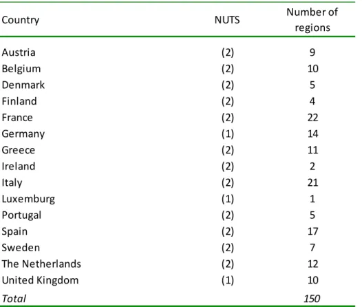
13 covariates.14 The final sample used for the empirical analysis covered 150 regions of the EU-15 countries, observed over the period 1990-2009. Table 1 shows the number of regions used for each country, according to the Nomenclature of Statistical Units (NUTS) and distinguishing between the NUTS1 and NUTS2. The choice to utilize both NUTS1 and NUTS2 was imposed by the necessity to match data from different sources. Indeed the
‘Farm Accountancy Data Network’ (FADN) regional classification does not always match
the NUTS2 level definition.
Dependent variable
Previous empirical applications computed the rate of out-farm migration simply as the growth rate in agricultural employment from one year to the next, disregarding the dynamics in the total labour force (see Barkley, 1990; D’Antoni and Mishra 2010). This approach can be a reasonable approximation when the exercise is conducted within a single country. However, working across the EU regions disregarding differences in total labour force dynamics can introduce a systematic bias in the inter-sectoral labour migration estimates.
To reduce this source of bias, we follow Larson and Mundlak (1997), assuming that, without migration, labour in agriculture and non-agriculture would grow at the same rate as the total labour force. Deviation from this rate is attributed to migration. Formally, the rate of out-farm migration is estimated using the following relation:
(3) � = [�� − + � − �� ] �⁄ � − ,
where � = � − � − ⁄�− is the growth rate of the total labour force.
Yet using (3) to estimate out-farm migration is not immune to potential shortcomings. A first drawback lies in the fact that it does not take into account part-time farming, an important characteristic of the EU agriculture. A second issue is that, to calculate
14 The dropped regions are Greater London (UK) and Ovre Norrland (Sweden). The first is a small urban
region with a population density of almost 5,000 inhab/kmsq (20 times the mean density of all other regions), and relative labour close to 500 (15 times the rest of EU regions). Ovre Norrland is a wide and poorly populated region located in the northern of Sweden where total CAP payments from FADN range between 1.1 and 3 times the farm valued added (more than 5 times what observed in the rest of EU regions). Given these extreme values they exert strong influence on the estimated coefficients and, especially, on the R-square of the regression, that increase from 0.25 to 0.53, after their removal. Note, however, that all the results reported in the paper are robust to the inclusion of these additional regions.
14 migration, we should use data on labour from census data. Unfortunately such data are only available every ten years. Thus, we were forced to use employment data to measure annual migration at the EU regional level.15 This variable is a good proxy of out-farm migration rate only if the (un)employment, the participation/activity rates and the age structure tend to be equal across sectors. But this is hardly the case as, for instance, the age structure differ significantly between agriculture and non-agricultural sector and such difference is likely to vary over time. So, it is implicit in the dependent variable definition that it is measured with error, a problem that cannot be controlled by simply introducing appropriate covariates.16 Thus, it will be important to test for the possible endogeneity induced by measurement errors, as discussed in the previous section.
The basic employment data used to measure the out-farm migration rate comes from
the Cambridge Econometric’s Regional Database based on Eurostat. During the observed period (1990-2009) the average rate of out-farm migration across the EU-15 regions has been about 2.5% per annum. This average value masks substantial heterogeneity both over time and, especially, across regions. The out-farm migration rate has been equal to 3.0% in the 1990-1999 period, going down to 2.1% in the 2000-2009. Interesting, the lower out-farm migration of the second decade is largely attributable to a value close to zero in 2008 and even slightly negative in 2009, probably as an effect of the 2008 commodities price spike, and of the 2009 global crisis.
Across regions, the net farm migration rate shows great variation (see Figure 1). In the observed period the migration rate is even negative for some UK regions, like North East (1.9%), London (1.7%), and Yorkshire (0.4%) as well as the Région de Bruxelles (3.8%). On the contrary, the strongest migration rate can be found especially in regions belonging to southern countries like the Principado de Asturia (7.2%), Galizia (6.6) and Comunidad Valenciana (5.2%) in Spain, Algarve (5.1%) in Portugal or Emilia Romagna (3.9%) and Campania (3.7%) in Italy. However, there are also several northern regions with an out-farm migration rate significantly higher than the sample mean, like those of Vastsverige (5.0%) in Sweden, Flevoland (4.4%) in Netherland and Vorarlberg (4.2%) in
15 Note, however, that previous papers faced the same issue (see Barkley, 1990; Larson and Mundlak, 2003; D’Antoni and Mishra 2010).
15 Austria. Thus, consistent with the expectation, there is a negative relationship between the level of development and the rate of out-farm migration, as less developed regions are still in structural transformation. However, this negative relation is quite weak.
Policy data
Given our main objective, how we measure the policy variables at regional level is a critical issue. Previous studies followed two main approaches: measuring a regionalized producer subsidy equivalent (PSE) as in Tarditi and Zanias (2001), Anders et al. (2004) and, more recently, Hansen and Herrmann (2012); using the Farm Accountancy Data Network as in Shucksmith et al. (2005), and by combining the same source with Eurostat Regio-New Cronos database, assuring to the former also a time variation, as in Esposti (2007).
In theory, the last approach is the most suited to our analysis where econometric identification is based on the within-region variation in CAP payments. Unfortunately it has two main shortcomings. First, Eurostat does not provide time series data at the regional level for all EU countries. Second, and more importantly, Eurostat data is based on agriculture sectoral series, hence they do not incorporate decoupled subsidies after 2005. Thus, their use would reduce the time coverage of the analysis, and would preclude the possibility of investigating the possible differentiated effect between coupled and decoupled payments, as well as the effect of Pillar II subsidies.
To overcome these issues, we adopted a new strategy measuring CAP payments starting from the FADN data at the regional level. For every region covered by the FADN,
the amount of payments received by the ‘average farm’ is available for each year over the period 1990-2009. The extent to which the average farm is representative of the farm population, the computation of the ratio between such farm CAP payments and the respective farm net income (inclusive of subsidies) offers then the possibility of computing a consistent regional level of farm protection due to different CAP policy measures.
Note that this approach is fully consistent with previous empirical exercises conducted on the US farm out-migration (see Barkley, 1990; D’Antoni and Mishra, 2010), where the effect of government payments is indeed identify by using the ratio between farm subsidies and the farm value added at an aggregated (country) level.
A key advantage of our approach is the possibility of disentangling the CAP total payments into their different components, distinguishing between coupled and decoupled
16 Pillar I payments, as well as agri-environmental payments, less favoured areas (LFA),
investment aids and a residual category called ‘other’ subsidies of Pillar II.17 Note that some of the latter payments were introduced before Agenda 2000, thus the “Pillar II” expression could be not fully correct. Nevertheless, we chose to use it to clearly and easily distinguish between CAP market subsidies and CAP structural policies.
Finally, it is important to emphasize that our policy variables capture only the subsidies component, but not the market “price support” component, of total CAP transfers. Because the market price support component was still in place though at a decreasing rate during the observed period, we cannot disregard its effect on farm migration.18 However, we want to stress that in our framework, the price component of CAP protection is controlled through the relative income term, ri. Indeed, to the extent to which the price support component of the CAP has an effect on agricultural income, it will act by reducing the agricultural relative income. Note that this is an important advantage of our framework with respect to papers working at more disaggregated territorial level, where, given the lack of data on farm income, they fail to control directly for both the relative income and the market price component of the CAP, thus introducing a potential bias in the estimation of the CAP subsidies effect on out-farm migration.
Other covariates
The inter-sectoral income differential is measured by the ratio of income in non-agriculture to that in agriculture (ri). Income is measured as per worker Gross Value Added (GVA) at constant and basic prices. For non-agriculture sector we used the difference between total GVA and GVA in agriculture, as well as for non-agricultural employment.19 The data for
17Pillar I includes: ‘total subsidies on crops’, ‘total subsidies on livestock’ and ‘decoupled payments’. Pillar II includes: ‘total support for rural development’ and ‘subsidies on investments’. Note however that, the sum of the components of Pillar II policies (agri-environmental payments, LFA payments, investment aids and
the residual category ‘other’ subsidies) it is slightly lower than the ‘aggregate’ Pillar II subsidies. This data incongruence is probably due to some reporting errors in the Pillar II subsidy components.
18 In fact, although the price policy component of the CAP has been largely dismantled after the Fischler
reform, price support still play a not marginal role in total CAP as an effect of tariffs protection at the border. For example, in 2009, 25% of the OECD total producer support estimates going to agriculture was indeed accounted for by market price support in the EU.
19 Harris-Todaro type models suggest wages as a measure of (relative) labour returns. However, many papers
investigating out-farm migration found that more robust results are obtained when relative income or productivity, instead of relative wages, are used. Mundlak (1979) and Larson and Mundlak (1997) justify this findings arguing that, for a long-run decision that involves expectations, such as the migration out of agriculture, income is considered a more informative measure of the future prospects than wages, since wages
17
GVAs and employment are from the Cambridge Econometric’s Regional Database. Note that, to identify the true effects of CAP payments on out-farm migration, we need to include not just the term ri, but its counterpart ̂�, that is net of the income effect induced by CAP payments. Otherwise, we are introducing in the equation a double counting that will bias downward (in absolute value) the CAP subsidy effect.
In principle, one can simply subtract from the agricultural value added at basic price the CAP subsidy component. However, this approach is not only difficult to implement with existing data, but it implicitly assumes that the transfer efficiency of CAP payments is 100%, an assumption not supported by the evidences (see OECD, 2001; Michalek et al.
2012). For this reason we measured the relative income net of CAP subsidies, ̂�, by simply regressing the CAP payments on the relative income variable, and then keeping the residuals from that regression.
The other control variables included in the vectors X are the following. First, following Larson and Mundlak (1997), we include the relative labour force calculated as the ratio of employments in the non-agricultural sector to that in agricultural sector. On one hand, the relative labour captures the absorption capacity of non-agricultural sectors. On the other hand, given the direction of structural change with economic development, having a high level of (relative) agricultural employment means more potential migrants out from the farm sector. Second, to control for search costs and the probability to find a job in the non-agricultural sector, we include the overall rate of unemployment, and a measure of population density, calculated as the total population over regional area in Km2. This variable accounts for several market conditions, in particular product and land markets (Glauben et al. 2006). Furthermore, it represents a rough proxy of the average ‘distance’ from urban areas. Third, we include a variable that measures the amount of farm family workers. The underline idea is that a higher number of family members working on the farm lower the exit rate (Breustedt and Glauben, 2007).
In addition, we also include a variable measuring country differences in labour market institutions, which is increasing with the rigidities of labour entry and exit. Specifically, we use the OECD employment protection indicator called “EP_v1” (see OECD, 2010).
are not the only component of farmer's income. They also note that measurement problems with wage data provide another reason to use relative income rather than relative wages.
18 This index is the average of 6 different sub-indices of “regular” and “temporary” contracts with a scale from 0 (less restriction) to 6 (most restrictions). The intuition is that higher labour rigidities should increase the costs of out-farm migration. Finally, to capture the reform’s effects not due to the level of payments, a dummy variable for Pillar I decoupled subsidies was included, taking the value of one in 2005-2009 and zero otherwise.
Information on population, regional area, unemployment rate, and total and sectoral
employment, comes from the Cambridge Econometric’s Regional Database. Differently,
information on farm family workers comes from FADN, while the labour institutions rigidity index is based on OECD data. Summary statistics of the variables explained above are reported in Table 2.
4. Econometric results
4.1 Static fixed effects modelTable 3 reports benchmark fixed effects estimates of equation (1), where we include different sets of variables to check for the robustness of the results.20 The estimated standard errors are clustered at the regional level, to account for heteroscedasticity and autocorrelation of unknown form.21 Augmented Dickey Fuller (ADF) tests were used to determine whether the variables were stationary. Results of the Maddala and Wu (1999) Fisher combination test and of the Im et al. (2003) test for unbalanced panel allowed us to reject the hypothesis that the variables were non-stationary (p-value < 0.01), with the exception of relative labour and unemployment rate.22 However, these variables become stationary in first difference. Thus, they were introduced in first difference in the static fixed effects specification, and as such they capture short-run effects.
In all specifications total CAP subsidies enter with a negative and strongly significant coefficient (p-value < 0.01) suggesting that, overall, CAP payments played a role in
20 We also tested several possible non-linearities in the relation between CAP payments and out-farm
migration, by adding interaction effects and square terms. However, these non-linearities turn out to be systematically insignificant. These additional results can be obtained from the authors upon request.
21 We test for spatial correlation with the Pesaran’ (2004) CD and Frees’ (2004) tests. While some (weak)
spatial correlation exists in the cross-sectional units, the robust clustered standard errors used in the regressions are virtually identical to those proposed by Driscoll-Kraay, that account for the presence of cross-sectional dependence.
22 The tests were carried out in Stata, by using the command xtunitroot and xtunitroot ips (both without trend),
respectively. To save space we do not report this additional ADF tests. However, they can be obtained from the authors upon request.
19 keeping labour force into agriculture, ceteris paribus. As expected, the CAP subsidies coefficient increases of about 30% passing from column 1 to column 2, where the relative
income term is ‘depurated’ of the double counting discussed above, then its magnitude
remains fairly stable across specifications.
In line with the labour migration model, the relative income between non-farm and farm sector exerts a positive and significant effect on the level of farm out-migration (p -value < 0.01). The estimated elasticity is about 1.1, thus smaller than the one estimated by Barkley (1990) for the US (equal to 4.5). This lower estimated elasticity suggests that at the EU regional level, farm out-migration is less responsive to income differences. Changes in the relative labour force were also strongly significant and positive. Thus, with positive difference in the labour force ratio from one period to the next, farm workers can be increasingly absorbed into the non-agricultural sector, resulting in greater migration of
labour from agriculture, a result close to the findings of D’Antoni and Mishra (2010). Regression 3 adds a battery of other covariates. Population density enters with the expected positive coefficient, but it is never statistically different form zero. Variation in unemployment display a positive coefficient, that is contrary to the common intuition, but it is never significant. Among the other covariates, farm family workers and the restrictiveness of labour protection institutions have the expected negative sign but are not significant. Instead, we find a strong negative effect of the Fischler reform dummy. We will return later to the interpretation of this effect.
In regressions from column 4 to 9, the effect of different CAP subsidies are investigated in great detail. First, column 4 splits the CAP subsidies into Pillar I and II payments. The estimated coefficient of Pillar I turn out to be negative and significant (p -value < 0.05), differently the effect of Pillar II payment is positive, although insignificant. The last result come to some surprise, as both anecdotal considerations and some previous empirical evidence (Pufahl and Weiss, 2009; Petrick and Zier, 2011) point in an opposite direction.
However, a closer inspection of the results in column 4 suggests the presence of some inconsistencies. Indeed, if the true effect of Pillar II subsidies is really positive, then it is difficult to understand why in regressions 3 the coefficient of total CAP payments is estimated with higher precision than when the coefficients of Pillar I and II are splitted. In
20 fact, whether problems of aggregation bias in CAP subsidies are at work, they should go exactly in an opposite direction, suggesting that the reason of these inconsistencies are elsewhere, and probably linked to collinearity problems. We will return shortly to this problem.
Column 5 further splits the CAP payments in each of the components considered. The coupled and decoupled payments of Pillar I exert significantly negative effects on out-farm migration as before. Differently, the effects of rural policy are strongly heterogeneous, being positive and significant for the agri-environmental and investment aids, and negative for LFA and other subsidies, though the coefficient of the last variable is insignificant. While the effects of investment aids and LFA payments make sense with respect to the common intuition (see the discussion in section 2), the same cannot be said about the positive effect of agri-environmental payments as such kind of subsidies should induce, at least in theory, more labour-intensive activities than the traditional ones.
To investigate whether multicollinearity is the reason of these counterintuitive results, we noted that the correlation coefficient between Pillar I and Pillar II subsidies (equal to 0.62) is not too high, although it is largely due to agri-environmental subsidies where it further rises to 0.67. However, the correlation of the estimated coefficients (not the variables) is 0.90, indicating possible collinearity problems. We checked more formally for collinearity using the variance inflation index (VIF).23 This test gives a clear indication that collinearity could be a problem and, in line with the counterintuitive evidence discussed above, suggests that the collinearity concern involves, almost exclusively, agri-environmental subsidies and Pillar I measures.
Thus, in columns 6-9, we re-run regressions including Pillar I and Pillar II subsidies separately. However, to reduce the potential omitted variables bias coming from these specifications, we measured our relative income term net of subsidies, just retaining in it the omitted specific policy variables. More precisely, in regression (6) the relative income
23 Allison (1999) suggests that problems can arise when VIF is higher than 2.5. In our regressions, when the
policy variables are entered separately as in regressions (6) and (8) of Table 3, the VIF is equal to 2.7 and 2.2 for Pillar I and Pillar II subsidies, respectively. By contrast, when they are entered simultaneously as in regression (4), the VIF of the two variables increases to 7.9 and 6.1, respectively. This implies that the Pillar I and Pillar II standard errors increase of about 2.6 times (root squared of VIF). In addition, when all the four Pillar II measures are introduced together, the collinearity concern involves, almost exclusively, agri-environmental subsidies, whose VIF strongly increases passing from 1.57 (regression 9) to 6.28 (regression 5).
21 is netted only by Pillar I subsidies, but not from the (omitted) subsidies of the Pillar II, and similarly for regressions 7-9. This is a second-best solution, but it gives us the possibility to have a better sense of the “true” policy effects.
First, considering Pillar I payments, not surprisingly the estimated policy effect is negative and significant, both in isolation (column 6), and when the effect between coupled and decoupled subsidies is splitted (column 7). Interestingly, now the magnitude of the estimated coefficients in absolute value decreases of about 25%-40%, and are estimated with great precision (p-values < 0.01). Second, when Pillar II subsidies are included in isolation (column 8), also this group of measures, taken as a whole, points to a strongly significant negative effect. However, once again this masks heterogeneity across instruments. Splitting Pillar II policies, we find that the effect of agro-environmental measures now switch to negative, being statistically significant at the 10% level. “Other payments” is again negative but not significant, while LFA maintains its negative and strongly significant effect. Finally, investment aids, consistently with the expectations, display a positive effect on farm out-migration. Broadly speaking, the results of Pillar II measures are more in line with the findings of Petrick and Zier (2011).
Summarizing, the results point to a robust negative out-farm migration effect of overall CAP subsidies, and of both coupled and decoupled Pillar I payments. The out-farm migration effect of Pillar II payments are, instead, less clear. On the one hand we find a significantly negative effect of LFA payments and a positive one for investment aids, a result quite robust across specifications. On the other hand, the effect of Pillar II payments as a whole category, and that of agri-environmental payments in particular, the most representative policy in term of money spent, are sensitive to the specifications. From these results one can raise a general issue of identificability of the CAP effects, suggesting that the separability between Pillar I and II effects appears problematic at this level of (regional) aggregation. One reason for this issue appears attributable to the strong overlapping between agri-environmental and Pillar I subsidies at the regional level. However, there is evidence that this it is not the only reason; otherwise would be difficult to understand why the estimated effect of agri-environmental subsidies remain weak also when the Pillar I
22 subsidies are dropped from the regression. Thus further work is needed to better understand the link between agri-environmental measures and farm labour.24
4.2 Dynamic panel model
Table 4 introduces dynamics into the specification, by estimating an autoregressive model using the DIFF-GMM estimator.25 The dynamic specifications are identical as in columns 6 to 9 of Table 3. However, now the policy variables are also treated as endogenous, using the t –2, t –3 and longer lags levels, as instruments. This strategy should shed further light on the robustness of our findings to measurement errors and other forms of endogeneity. Moreover, by instrumenting the policy variables we further reduce the omitted variable bias due to the difficulty of including simultaneously Pillar I and Pillar II payments.
Standard tests to check for the consistency of the DIFF-GMM estimator (see Roodman, 2009) are reported at the bottom of Table 4. The Arellano-Bond test for autocorrelation indicates the presence of first order serial correlation but does not detect second-order autocorrelation. Hence, under this circumstance the OLS estimator is inconsistent, while the use of a dynamic GMM specification is correct. Moreover, the standard Hansen tests for the suitability of the instruments confirm that our set of instruments is valid.
The coefficient of the lagged dependent variable is significant and negative, although its magnitude is quite low (around 0.08). A negative autocorrelation coefficient means that if the migration rate at time t –1 is high, then it will be slightly lower at time t, a result consistent with the adjustment process under study.
The results of the DIFF-GMM estimator present some important differences with respect to the static model of Table 3. First, here the relative labour ratio affects negatively the migration rate and it is strongly significant. Although the specification is different from
24 A possible interpretation of the weak effect of agri-environmental payments on farm labour, can be found
in the results of Nilsson and Johansson (2013) and Kilian et al. (2012) on land values in Sweden and Germany, respectively. These authors showed that agri-environmental payments are negatively correlated with land prices. Thus, if land value is an important determinant of farm out-migration decision, as argued by Barkley (1990), then our results are not so surprising.
25 Because it is reasonable to assume that a reduction in CAP payments at time t will produce an effect at
time t + n, we also experimented with an autoregressive distributed lag model, by adding CAP payments with lags higher than 1. However, for both total subsidies and Pillar I and II subsidies, lags higher than 1 are systematically insignificants.
23 the static model, and thus not fully comparable, the result is consistent with the idea that the larger is the labour force in agriculture relative to the non-agricultural sector, the more farm out-migrants can be expected, namely regions tend to converge to a similar level of relative labour ratio. Second, and in line with the a priori expectation, in the dynamic model the unemployment rate negatively affects the rate of out-farm migration and is almost always significant at the 5% level. Third, in line with the intuition, the population density is now positive and strongly significant.
Moving to the policy variables, their estimated coefficients are always negative and, for the most part, statistically significant giving broad confirmation of the static results. Starting from total CAP subsidies, the magnitude of the estimated coefficient is nearly identical to the static model (–0.0129 vs. –0.0127) when the variable is treated as exogenous (column 1). However, it increases in absolute value to –0.0168 (p-value < 0.01) when the policy variable is treated as endogenous (column 2). Hence, even if measurement errors in the dependent variable can be a potential problem, if anything, their net effect would point to a reduction rather than to an overestimation of the absolute magnitude of the policy effect on farm out-migration.
Columns 3 to 6 consider Pillar I policies. The magnitude of the estimated coefficients is, once again, closed to the static model, and it increases slightly when the variable is treated as endogenous (column 4). However, when we split the effect between coupled and decoupled subsidies (columns 5-6), the latter is no longer significantly different from zero when treated as endogenous (column 6). Thus, the evidence of a negative out-farm migration effect of decoupled payments is weak in this dynamic specification.26
The picture of the effects on the out-farm migration changes significantly when we consider Pillar II policies (columns 7 to 10). In this case the absolute magnitude of the estimated coefficients for Pillar II subsidies shows a slight increase on passing from the static to the dynamic specification (–0.021 vs. –0.025), or when the policy variable is endogenized (see column 8). When we split the effect of Pillar II policies in its components, the direction of the effect is always similar to those of the static model, but only investment
26 Note however that, given the data structure, this result is not so surprising. In fact, for 2005 and 2006, the
t – 2 instruments for decoupled subsidies are zero. Thus, the identification relies only on the last three years observations.
24 aids remain always significant at the 5% level. Differently, agri-environmental payments are significantly negative only when the variable is treated as endogenous, and LFA payments are significantly negative only when they are considered as exogenous. Thus, overall, the effects of Pillar II payments are less robust and quite sensitive to the specification.
Finally, the Fischler reform dummy is once again negative and significant in all the specifications.”This result is puzzling. In fact, first of all it is contrary to the findings of Petrick and Zier (2012) who found evidence that the introduction of decoupling in 2005 led to labour shedding in three East German Landers. By contrast, our results point to a
decrease of farmer’s decision to exit agriculture, although the estimated elasticity of decoupling subsidies is lower than that of coupled ones (see below). A possible reason for this counterintuitive result can lie in the commodities price spike of 2007 and 2008. Indeed, commodity prices started to rise slowly already in 2005-2006, thus with a partial overlapping with the Fischler reform effect.
4.3 Magnitude of the estimated effects
So far, we have not yet properly discussed the magnitude of the estimated policy coefficients. A consistent comparison between the out-farm migration effects of different CAP policies can be made on the basis of their respective elasticities (Table 5).27 Several interesting patterns emerged. First, a 1% increase in total CAP payments decreases out-farm migration by about 0.172% when the effect is estimated using the static fixed effects model, such value rises to 0.190% and 0.246% when dynamics and endogeneity are accounted for. Thus, the magnitude of the overall economic effect is rather moderate, but it increases when dynamics and endogeneity are taken into account.
This average effect cancels out relevant differences across CAP instruments. The long-run elasticity of Pillar I payments, equal to about 0.274% when dynamics and endogeneity are considered (see columns 3), is indeed about 2.7 times higher in absolute value than the elasticity of Pillar II policies. Within Pillar I, the coupled payments display a higher
27 The elasticities are estimated at the sample mean using the following formula: �ln �ln =
̅
��
̅��, where ̅�
and �̅� are, respectively, the sample mean of the specific CAP subsidy and of farm out-migration, while is the estimated marginal effect of the CAP subsidies. For the long-run elasticity, the coefficient is divided by one minus the coefficient of the lagged dependent variable.
25 absolute elasticity than decoupled payments, while across Pillar II instruments, investment aids display the higher absolute elasticity to out-farm migration. Thus from the value of the above elasticities, one can conclude that if the labour effect of CAP payments is ranked high in the policy agenda, then the most effective policy tools to reach this objective should be coupled payments, followed by decoupled payments, ceteris paribus.
Another way of interpreting the economic magnitude of our findings, is through a back-of-the-envelope calculation. According to the parameter estimates in column (1) of Table 5, a marginal increase in the explanatory variable “total CAP payments” lower the dependent variable by 0.0129 points. Using the average CAP subsidy value across the panel (that is 0.331, see Table 2) and multiplying it for the parameter estimates (0.0129) we obtain 0.0046, that is the reducing average effect of CAP subsidies in terms of out-farm migration. Multiplying such value for the average stock of agricultural workers (6.436 millions/year), we can obtain a rough estimate of the flow of out-farm migration prevented by CAP payments, which are around 27,000 agricultural workers per year. To render such value in percentage consider that, without subsidies, the annual out-farm migration rate would increase from the actual 0.0255 to 0.0295. The effect of CAP payments, then, reduces the rate of farm labour migration by around 14.3%, thus not an irrelevant number.28 Finally, taking into account the confidence interval around that point estimate, the percentage reduction of the rate of out-farm migration attributable to the CAP subsidies is still positive, ranging from a minimum of about 6% to a maximum of 20%. A conservative view is thus to interpret this calculation saying that CAP subsidies might generate a reduction of out-farm migration, although the effect can be rather moderate.
6. Concluding remarks
Understanding the effect of CAP policies is important as a deeper comprehension of their incidence would allow the design of better policies. This paper contributes in this direction by studying how different CAP subsidies affected out-farm migration across 150 EU regions over the 1990-2009 period. Within the standard neoclassic two sectors model,
28 There are several caveats behind this calculation. For example, about the consequences, we are assuming
that the effect is fairly homogeneous across regions. However, relaxing this assumption would be beyond the scope of our analysis