The Effects of Additive Outliers and Measurement Errors when Testing for Structural Breaks in Variance

Estudos e Documentos de Trabalho

Working Papers

11 | 2010

THE EFFECTS OF ADDITIVE OUTLIERS AND MEASUREMENT ERRORS WHEN TESTING FOR STRUCTURAL BREAKS IN VARIANCE

Paulo M. M. Rodrigues Antonio Rubia

June 2010

The analyses, opinions and fi ndings of these papers represent the views of the authors, they are not necessarily those of the Banco de Portugal or the Eurosystem.

Please address correspondence to

Paulo M. M. Rodrigues Economics and Research Department

Banco de Portugal, Av. Almirante Reis no. 71, 1150-012 Lisboa, Portugal; Tel.: 351 21 313 0831, [email protected]

BANCO DE PORTUGAL

Edition

Economics and Research Department Av. Almirante Reis, 71-6th

1150-012 Lisboa www.bportugal.pt

Pre-press and Distribution

Administrative Services Department Documentation, Editing and Museum Division Editing and Publishing Unit

Av. Almirante Reis, 71-2nd

1150-012 Lisboa

Printing

Administrative Services Department Logistics Division Lisbon, June 2010 Number of copies 170 ISBN 978-989-678-029-6 ISSN 0870-0117 Legal Deposit no. 3664/83

The E¤ects of Additive Outliers and Measurement

Errors when Testing for Structural Breaks in

Variance

Paulo M.M. Rodrigues

y

Banco de Portugal

Universidade Nova de Lisboa and CASEE

Antonio Rubia

z

Department of Financial Economics University of Alicante

Abstract

This paper discusses the asymptotic and …nite-sample properties of CUSUM-based tests for detecting structural breaks in volatility in the presence of stochastic conta-mination, such as additive outliers or measurement errors. This analysis is particu-larly relevant for …nancial data, on which these tests are commonly used to detect variance breaks. In particular, we focus on the tests by Inclán and Tiao [IT] (1994) and Kokoszka and Leipus [KL] (1998, 2000), which have been intensively used in the applied literature. Our results are extensible to related procedures. We show that the asymptotic distribution of the IT test can largely be a¤ected by sample conta-mination, whereas the distribution of the KL test remains invariant. Furthermore, the break-point estimator of the KL test renders consistent estimates. In spite of the good large-sample properties of this test, large additive outliers tend to generate power distortions or wrong break-date estimates in small samples.

JEL Classi…cation: C12, C15, C52

Keywords: additive outliers, variance homogeneity, CUSUM-type tests

We thank Javier Gómez-Biscarri, Uwe Hassler, Enrique Sentana, and seminar participants at the Humboldt University of Berlin, and conference participants of the 31th SAE Conference (Oviedo), XIV Finance Forum (Castellón) and the 2nd Congress of the Italian Empirical Economics and Econometrics Society (Rimini) for comments and suggestions. Any remaining error is our own responsibility. Financial support from POCTI/ FEDER (grant ref. PTDC/ECO/64595/2006) and the Spanish Deparment of Education and Science (grant ref. ECO2008-02599/ECON) is gratefully acknowledged.

y_{Banco de Portugal, Economics and Research Department, Av. Almirante Reis, 71-6th ‡oor, 1150-012}

Lisbon, Portugal (e-mail: [email protected]).

z_{University of Alicante, Campus de San Vicente, CP 03080, Spain. Tel/Fax. (34) 965 90 36 21.}

1

Introduction

There is much evidence that economic time-series are non-stationary when observed over long periods of time. Policy-regime shifts and exogenous factors may generate parame-ter instability in the underlying generating process, often leading to abrupt changes in time series dynamics. Recent literature in Financial Economics has addressed variance homogeneity, …nding strong evidence of instability; see,e.g., McConnell and Perez-Quirós (2000), Sensier and van Dijk (2004) and references therein. This topic is particularly important in …nancial markets because the second-order moment is central to Financial theory and its empirical applications.

The most popular statistical methods speci…cally designed to detect breaks in volatil-ity are CUSUM-type tests. Into this category fall, among others, the tests by Pagan and Schwertz (1990), Inclán and Tiao (1994), Kokoszka and Leipus (2000), Chen, Choi and Zhou (2005), and Deng and Perron (2008a, 2008b). The ability of the CUSUM tests to identify structural changes depends critically on the empirical realism of the underlying assumptions. The most remarkable features of …nancial data include the existence of time-varying volatility patterns, and a tendency to generate abnormally large observations that cause similar e¤ects as additive outliers.1 _{Andreou and Ghysels (2002) illustrate the}

per-vasive e¤ect of persistent volatility on CUSUM tests experimentally. However, distortions that may arise from extreme observations, or other forms of stochastic contamination, have, to the best of our knowledge, not been addressed yet in the literature.

In this paper, we formally discuss the e¤ects that sample contamination has on the asymptotic properties of CUSUM-type tests for detecting change points in variance and characterize the …nite sample behavior by means of Monte Carlo simulations. Our theo-retical discussion follows in a general framework in which additive outliers and/or mea-surement errors are treated as particular cases aiming to analyze the e¤ects on i) the asymptotic distribution, ii) the consistency of the turning point estimator, and iii) the small-sample performance of CUSUM tests. Owing to their empirical relevance, special focus is placed on two well-known tests, but it should be stressed that the main conclusions are directly extensible to most testing procedures which are based on this framework. In particular, we study the parametric test suggested by Inclán and Tiao [IT] (1994), and the non-parametric generalization proposed by Kokoszka and Leipus [KL] (2000). These tests have been extensively applied on …nancial data; see, among others, Aggarwal, Inclán and Leal (1999), Andreou and Ghysels (2002, 2004), and Cuñado, Gómez-Biscarri and Pérez de Gracia (2006).

The results of our analysis can be summarized as follows. First, the IT test is not asymptotically invariant under stochastic contamination. It is biased towards serious overrejection – even in large samples – owing to the use of conservative critical values. In contrast, the non-parametric correction of the KL test ensures invariance and renders consistent estimates of the break-date. Our analysis reveals patterns which would be hard to explain in the absence of a formal theoretical analysis. For instance, the distribution of the IT test is more sensitive to a small likelihood of outliers than to a large probability of them, which is exactly the relevant case for empirical applications. Similarly, the asymptotic robustness of the KL test is not obvious a priori, since additive outliers may 1_{Outliers are discordant observations that seem to be far beyond the process that rules most}

obser-vations. In …nancial markets, outliers are linked to rare shocks not related to the trading process, or abnormal ‡ows of information arrivals. A well-known example is the market crash in October 19, 1987.

introduce asymptotic bias in least-squares based methods. In spite of the correct large-sample properties, using Monte Carlo analysis we observe that the KL test may su¤er important power distortions in …nite-samples when extreme outliers are present, which provide simple and straightforward reasons to explain the contradictory …ndings whenever the IT and KL tests are simultaneously applied (see, for instance, the analysis in Cuñado

et al., 2006, on data from emerging markets). Neglected outliers tend to bias the IT test

towards …nding a large number of breaks, whereas the KL test exhibits low power and tends to …nd few or no breaks at all.

The rest of the paper is organized as follows. Section 2 brie‡y outlines the test statistics which are analyzed in this paper. Section 3 derives the asymptotic properties under sample contamination, and provides a set of su¢ cient conditions to justify the results. Section 4 reports Monte Carlo results, which illustrate the small-sample behaviour of these tests and discusses the performance of the procedures in addressing variance homogeneity for US monthly stock returns. Section 5 summarizes and concludes. Finally, a technical appendix collects the proofs of the theoretical results presented in the paper.

2

Testing for structural breaks in variance

Assume that _frtgT_t=1 is the realization of a (zero-mean) stochastic process that veri…es some restrictions which will be discussed later. The null hypothesis, H0 : V ar(rt) = 2 with 2 constant over the entire sample, is tested against the alternative of single or multiple breaks of unknown location. The usual testing procedure infers the most likely break-position endogenously through cumulative sums of squared observations; r2

t;as they provide an unbiased estimate of the unconditional variance. The key statistic is

DT (k) = " _k X t=1 r_t2= T X t=1 r2_t ! k=T # ; k= 1; :::; T; (1)

which can be viewed as an approximate likelihood ratio under some conditions. Under the alternative of a single break, the estimator of the break-date, say bk;is determined as

argmaxkjDT (k)j. Whether this estimate is signi…cant or not is then addressed through a test statistic based on DT(k) whose asymptotic distribution can be characterized as the

supremum of a standard Brownian Bridge (SSBB henceforth) under suitable restrictions.

2.1

The Inclán and Tiao [IT] test

The IT test is a natural extension of CUSUM-type tests in regression models for the detection of shifts in variance, de…ned as

IT =pT =2arg max

1 k T j

DT(k)j: (2)

Inclán and Tiao (1994) show that if,rt iidN(0;1); thenIT converges weakly to SSBB as T _{! 1}. The IT test is initially intended to estimate the location of a single break as

b

k = arg max1 k T jDT (k)j: However, a more general procedure based on the successive computation of(2)and the corresponding break-date estimation to gain power against the alternative hypothesis of multiple breaks can be considered. In particular, Inclán and Tiao

(1994) suggest the so-called Iterative Cumulative Sum of Squares (ICSS) method, which embeds the basic algorithm into an iterative scheme based on successive computations of

(2)on di¤erent segments of the series, which are consecutively determined after a possible change point is detected.

2.2

The Kokoszka and Leipus [KL] test

The KL test statistic is de…ned as a suitably re-normalized version ofDT (k); namely,

KL=T 1=2_Mc_4;T1=2arg max 1 k T j GT (k)j (3) with GT(k) Pk_t=1rt2 k T PT t=1r 2

t and Mc4;T being a consistent estimator of the long-run variance of r_t2 E(r_t2); i.e., the limit of _T1EhP1_t=1(r_t2 E(r_t2))2i; say _M4 < 1: Since GT (k) = DT (k)

PT t=1r

2

t; and noting that b 2 T 1PT_t=1r2_t; it follows that KL= s 2_b4 c M4;T IT: (4)

The main purpose of the KL test is to weaken the Gaussian iid restriction of the IT test by using a model-free setting. Under fairly general conditions which do not hinge upon the particular distribution of the data, _M4 can be estimated consistently using non-parametric techniques. Thus, the asymptotic distribution of the KL test is SSBB. The break-point estimator is de…ned as bk = arg max1 k T jGT(k)j; which is equivalent toarg max1 k T jDT (k)j:Therefore, as in the IT test, the KL test can also be embedded into the same ICSS algorithm to gain power against multiple breaks.

3

Asymptotic theory

Consider …rst a data generating process [DGP] in which the main signal is perturbed with a stochastic contamination process that generates additive outliers and/or measurement errors, characterized under suitable restrictions. The objective is to de…ne a process with similar statistical properties as those commonly found in …nancial and other economic time-series and to keep the assumptions to a minimum possible.

Assumption A1. The observable data, _frt; t 1g; is generated from

rt= +"t+ t+Bt[ + vt] (5)

where is some …nite constant, "t is the regular component and tand Zt Bt[ + vt];

are di¤erent sources of stochastic contamination.

Assumption A2. The stochastic contamination components _f t; Ztgobserve the

follow-ing properties:

i) The measurement-error generator _{f t}; t 1_g is independent of "t and Zt, and t

iid 0; 2 _{for some …nite 0: Also, E(}

j tj4+ )<1 for some >0:

ii)The additive-outlier generator _fZt; t 1g;is independent of "tand t;with Btbeing a

vt iid(0;1) such that E(jvtj4+ ) < 1 for some > 0; 0 p < 1, 0 < < 1; and

0< <₁:

Assumption A3. The regular component _f"t; t 1g observes the following properties:

i) E("t) = 0; E("2t) = 2" <1.

ii) suptE(j"tj4+ )<1 for some 0:

iii) "t is strong mixing with mixing numbers mj satisfying P_j1₌₁ms=j (s 2) < 1 for some

s >4; and limT!1 E h T 1₍P_["2 t 2"]) 2i M" 4, with 0<M"4 <1:

Assumption A3’. Let _Ft be the -…eld generated by f"t; Zt; t; "t 1; Zt 1; :::g: Then

f"t;Ftg1t=1is a strictly stationary and ergodic martingale di¤erence process and E(j"tj4+ )<

1 for some 0:

Assumption A4. "t is independent of f t; Ztg:

Some comments follow. Assumption A1 sets the basic DGP, in which measurement errors (ME) and/or additive outliers (AO) lead to the impossibility of observing the true signal"t.2 In the …nancial literature,Zt is usually referred to as a (discrete-time) stochas-tic jump process. In the econometric literature, a number of papers have focused on the e¤ects of AOs through restricted forms of this general speci…cation; see,e.g., Franses and Haldrup (1994), van Dijk, Franses and Lucas (1999) and Vogelsang (1999). Assumption A2 assumes that AOs are generated independently of the regular component, which seems accurate for …nancial returns, as it captures extreme events which are unrelated to the normal trading process but which nevertheless are able to in‡uence the observable series. Similarly, the ME component is assumed to be exogenous, which does not seem a particu-larly restrictive condition in practice. Since _tandZt are bounded in probability,"tis not perturbed by arbitrarily large values.3 Condition A3 is fairly general and standard in the literature. It allows for …nite-order ARMA structures and/or several time-varying volatil-ity processes, such as stationary GARCH-type and stochastic volatilvolatil-ity models. Condition A3’may be su¢ cient when the series are uncorrelated but not independent, as is mostly the case in …nancial time-series. Finally, A4 is a maintained assumption in related studies, such as Franses and Haldrup (1994) and van Dijk et al. (1999). Its practical purpose is to allow us to analyze the e¤ects of stochastic contamination in a model-free framework. We shall comment on the e¤ects of weakening this assumption later on.

3.1

Asymptotic distribution of the test statistics

In this section, the asymptotic distributions of the IT and KL test statistics under additive outliers and/or measurement errors are formally derived. We denote ‘₎’ as the weak convergence of probability measures in D[0;1], ‘_!p ’as convergence in probability, W( )

represents a standard Wiener process on ₂[0;1]; W ( ) =W( ) rW(1)is a standard Brownian Bridge,[ ] is the integer function, and tr( ) denotes the trace of a matrix.

2_{It is widely accepted that AOs are part of the return’s generating process. Non-synchronous and}

thin-trading may generate measurement errors, particularly, in data recorded from emerging markets.

3_{Alternatively, a more extreme (but somewhat less general) form of contamination in which outliers}

are allowed to be arbitrarily large could be considered as well. The analysis of the performance of the CUSUM tests, and the formalization of robusti…ed alternatives, constitute interesting topics for future research. We thank an anonymous referee for bringing this issue to our attention.

Lemma 3.1. De…ne the random vector t = "2t; Zt2; 2

t;2"tZt;2"t t;2 tZt

0

and assume

A1-A4 hold true. Then, as T _{! 1}, p1

T

P[T ]

t=1 ( t E( t)))

1=2_{W( )in D[0;1]}6 and

uniformly in ₂[0;1]; where W( ) is a multivariate standard Wiener process with

co-variance matrix =_f!iig; !11=M"4; !22=p 4 2+ 4 v4 + 2 2 (3 + v 3) 2 ; !33 = 4 2; !44 = 4 2"p 2 + 2 ; !55 = 4 2" 2; !66 = 4 2" 2; and !ij = 0 for i6=j; where E("2 t) = 2"; vj =E v j t , j =E v j t :

Lemma 3.2. Denote ~rt =rt bT, where bT is a

p

T-consistent estimator of . Under the

conditions of Lemma 3.1, as T _{! 1};it can be established that (i)p1

T P[T ] t=1 [~r 2 t E(r2t)]) M14=2W( ) ;(ii)p1_T PT t=1[~r 2 t E(r2t)]) M 1=2 4 W(1)and (iii) T1 PT t=1r~ 2 t p ! 2 "+p 2₊ 2 ₊ 2_{;for any r} 2[0;1]; where _M4 V ar(rt2 E(rt2)) =tr( ):

Lemmas 3.1 and 3.2 state the convergence of the functionals involved in the IT and KL tests and clarify the dependence on the main driving parameter (see the technical appendix for details). The following theorem presents the asymptotic distribution of the tests.

Theorem 3.1. Let the IT and KL test statistics be de…ned as in (2) and (3),respectively,

and let _Mc4;T be a consistent estimator of the long-run variance M4. T hen, under the

conditions of Lemma 3.1 and as T _{! 1};

IT ₎ M 1=2 4 p 2 2 "+p 2 +p 2+ 2 sup 2[0;1]j W ( )_j (6) KL ₎ sup 2[0;1]j W ( )_j:

Corollary 3.1. If only additive outliers contaminate the sample, then Theorem 3.1

triv-ially holds with = ₄ = 0;whereas if only measurement errors are present, i.e., p =0,

then Theorem 3.1 trivially holds by setting all parameters related to the AOs equal to zero.

The proofs of Theorem 3.1 and its corollary follow directly from Lemmas 3.1 and 3.2 and the continuous mapping theorem (see the appendix). Theorem 3.1 states formally one of the theoretical results of this paper, and has important implications for empirical purposes. The asymptotic distribution of the IT test is not invariant and it turns out to be heavily in‡uenced by the characteristics of the contamination process, since this introduces non-Gaussian features, such as excess kurtosis. The critical values from the correct asymptotic distribution will be larger whenever tr( ) > 2E(r2

t) 2

, and smaller otherwise. Since, the characteristics of the contaminating process are not observable, the IT test becomes infeasible under outlying observations and/or measurement errors. In sharp contrast, the KL test is scaled with a non-parametric HAC-type estimator of the long-run variance that succeeds in making the procedure robust to contamination, ensuring its convergence to the SSBB. Vogelsang (1999) …nds similar results in the di¤erent context of unit root testing, suggesting the use of the Phillips-Perron test procedure (which builds on the autoregressive spectral density estimation of the long-run variance parameter) to deal with AOs.

Remark 3.1: The diagonality of the asymptotic covariance matrix which characterizes

measurable function of"t, sayV1("t);and lagged values of a functionV2(Zt; t), provided conditions A3 or A3’are still ful…lled. Relevant examples of_V1 andV2 in this context are quadratic and absolute-value functions, given that the volatility process may be a¤ected by lagged outliers. De…ne t= t E( t)and let = limT!1 T1E

PT t=1 t

PT

t=1 0t : If A4 is replaced by the assumption that is a …nite positive de…nite matrix such that

= 0_{, then it follows as T ! 1 that p}1

T

P[T ]

t=1 t ) W( ); with this result

generalizing Lemma 3.1 in an obvious way. The diagonal elements of are those

of ; whereas the (non-zero) o¤-diagonal elements of this matrix depend speci…cally on the covariance structure related to _V1 and V2, and hence are model-dependent. It also follows that p1

T P[T ] t=1 [~r 2 t E(rt2)] ) 10 W( ); and T1 PT t=1r~ 2 t p ! 10E( t 0t)1;

with 1 being a conformable vector of ones. As in Theorem 3.1, it can be shown that

IT _{) V1;V2}sup _2[0;1]jW ( )_j; with _V1;V2 = p10 ₁ p_{2 (1}0_E(

t 0t)1) 1

; and again

KL ₎sup _2[0;1]jW ( )_j: This issue will be analyzed more carefully in the Monte Carlo section.

3.2

Consistency of the change-point estimator

We now discuss the ability of the tests to consistently estimate the location of an unknown turning point under the alternative hypothesis. We initially assume that only a single break a¤ects the dynamics of the regular component "t, as there is no practical sense in considering breaks in the contaminating structure. It is also necessary to make additional assumptions to characterize the nature of the structural break and introduce further notation. Denote ; 0< <1; as the break fraction, such that a shift occurs at time

k + 1; k = [T ]; and let "1t =f"tg_tk₌₁ and "2t =f"tgT_{t=k +1} be the pre- and post-break sub-samples such that E("2_1t) = 2_1" and E("2_2t) = 2_1"+ > 0: The break is of (…nite) magnitude and may be originated in the conditional or unconditional variance of the regular series. In both cases, the shift in the variance of "t leads to a shift of the same magnitude in the variance of rt, i.e., =Var rt;t [T ] Var rt;t>[T ] : This property allows testing for changes in the unobservable component "t using the observed series

rt instead, but introduces ine¢ ciency. Note that both the IT and KL test procedures yield the same break-fraction estimation, namely _b = T 1arg max1 k T jDT (k)j. Our interest is to analyze if_b!p under the set of assumptions considered and the following additional condition.

Assumption A5. The sequence _f"tg1_t=1 veri…es i) suptE("4t) < 1 for all t, and ii) Cov "2_t; "2_j =O jt jj for all 1 t; j T and some 0 <1:

Condition A5 is embedded in A3 or A3’ when there are no breaks. With i) we rule out shifts which dramatically change the statistical properties of the process as considered under the null, such as parameter instability leading to diverging moments up to the fourth order. Condition ii) restricts the covariance structure of the time-series. Although "t is not stationary under parameter instability, we still require that the covariance between distant observations decays towards zero at a suitable rate. Note that ii) holds trivially for independent series, as well as for short-memory series. More importantly, ii) may be weakened considerably, as consistency can be proven under the more general condition

limT!1T 2 PT t=1 Pt jCov " 2

and allows for di¤erent rates of decay in the covariances. Convergence in probability for the estimator_b is provided as a theorem below.

Theorem 3.2. Consider _frtgT_t=1 as de…ned in A1 such that A2 and A4 hold true. Assume

that the unconditional variance of the regular component shifts from 2" to 2" + > 0;

0 < _{j j} < ₁; at some time k = [T ] for some ₂ (0;1) such that A5 holds true.

Let _b = T 1_{arg max}

1 k T jDT (k)j. Then, for an arbitrary >0 and some constant C

it follows that

Pr (_{jb j}> ) C

2 2p_T (7)

and, therefore, _b!p as the sample size is allowed to diverge.

Remark 3.2: Consistency holds for any estimator based onarg max1 k T jDT (k)j:If we

allow for cross-dependences, as in Remark 3.1, then_b!p holds generally if suptE("4t)<

1 and limT!1T 2PTt=1

Pt

jCov r 2

t; rj2 = 0.

The proof of consistency uses the Hájek-Rénji inequality in Kokoszka and Leipus, (2000), see the appendix for details. For a …xed shift ; the bias _{jb j} can be shown to be Op(T 1) and, therefore, b is super-consistent, a standard result in this literature. Consistency guarantees that the KL test not only uses the correct critical values, but also that these are applied on the correct location when the sample grows unbounded. Furthermore, Theorem 3.2 provides insight on how the representative characteristics of the DGP a¤ect the bias. In particular, the degree of serial dependence, the time of the break, and the excess of variability generated by the contaminating process increase the size of

C and will make it more di¢ cult to locate the break-position correctly in …nite samples (see appendix for further details). On the other hand, the sample size and the magnitude of the shift help to reduce the bias. This statistical tension completely disappears when

T _{! 1}; but (7) indicates the sources of small sample distortions for …nite T. This issue will be studied in greater detail in the Monte Carlo section below.

The extension of the single-break analysis towards the detection of multiple changes in variance is usually done through the ICSS algorithm suggested by IT; see Chenet al. (2005). The procedure starts by applying the single break-point detection over the entire sample. If a break is detected, the whole sample is divided into two subsamples, and the testing procedure is applied again in each subsample. The process is repeated until no changes are detected, yielding an estimate of the number of breaks, say m_b. Since, from Theorems 3.1 and 3.2 the KL test consistently estimates and identi…es a single break-point, the ICSS algorithm based on this test will also consistently estimate the unknown number of breaks, say m; in the multiple break context. We provide this result as a proposition below (the proof follows along the lines in Bai, 1998, and is therefore omitted to save space).

Proposition 3.1: Suppose that the conditions in Theorem 3.2 hold true and that there

is a number m < T of shifts in the unconditional variance of the regular process. In

particular, assume that for any j = 1; :::; m, the variance shifts from 2" to 2"+ j >0;

j jj < 1; at time kj = T j ; j 2 (0;1); such that kj kj 1 (k0 0) includes a

non-trivial set of observations, and A5 holds true. Let m_b be the number of breaks inferred

4

Finite-sample analysis

4.1

Monte Carlo analysis

Given its relevance, and in order to save space, in this analysis we center our attention on additive outlier e¤ects and focus only on the single-break case. Several experiments are considered to study possible small-sample size departures related to outliers when the regular component is A) an iid process, and B)exhibits time-varying volatility patterns. In addition, C) we also address the consistency of turning point estimation in small-samples.

A) Empirical size: additive outliers and independent observations.

We …rst assume that the regular component"tis iid to isolate the e¤ects of outliers. We generate simulated paths forrt="t+Bt[ + vt]; "t= t;with t andvt iidN(0;1): The discrete variable _Bt= ( 1;1;0) with the grid of probabilities p=f0;0:01; :::;0:50g; and increments of 0:01is used. We set _{2 f}0:5;1; :::;5_g;and increments of 0:5;covering a wide set of values including many relevant ones for empirical purposes. We initially set

= = 1:The sample size isT = 1000and we repeat the simulation process 25000 times for any combination of the analyzed values. The IT and the KL tests are computed using the simulated series, and the corresponding statistics compared to the 95% percentile from the SSBB (i.e., 1.36). The rejection rates of the null hypothesis are depicted in Figures 1 and 2.

[Insert Figures 1, 2 about here]

As discussed in the theoretical section, the distribution of the IT test is strongly a¤ected by the parameters that characterize the dynamics of the outlier process. We observe that extreme values lead to large size departures, specially for large, infrequent values (small pand large ), which is precisely the type of process that is to be expected in real …nancial data. These values generate large excess kurtosis and lead the IT test to over-reject.4 Although not reported here, in order to save space, the distortion in size ampli…es as increases (given that kurtosis depends on this parameter as well). In contrast, the KL test shows a ‡at, uniform distribution for the empirical rate of rejection which does not depend on nuisance parameters.

B) Empirical size: additive outliers and time-varying volatility.

We now turn our attention to the case in which the regular component exhibits time-varying volatility patterns. Owing to its empirical relevance, we assume that "t follows a GARCH(1,1) model, such as

rt = t t+Zt; t iidN(0;1) (8) 2 t = !+ 2 t 1+ 2 t 1;

as a function of the variable t: In the context of outliers, there are two possible speci…-cations, depending on whether they a¤ect the level of the series (level outliers), or a¤ect both the level and the variance (volatility outliers). In the …rst case, 2

t is independent of 4_{Relatively large values ofplead to undersized tests. This may seem surprising, but from the analysis}

of Theorem 3.1 we note that large values ofplead totr( )<2E r2

t

2

, hence undersizing the test. Such a degree of heterogeneity, however, is unlikely observed in practice.

Zt; and therefore we set t= t t "t. Thus, observed returns result from the convolu-tion of a jump-process and a standard GARCH model. This is the case explicitly studied in the theoretical section, and the DGP considered in most empirical applications. Alter-natively, if 2

t is also perturbed by AOs, then t = rt and the GARCH model includes jumps, a far more complex type of non-linear volatility process. We shall analyze both possibilities in our simulations.

First, consider the level-outlier case with AOs a¤ecting only the conditional mean.

We normalize the unconditional variance to unity by setting ! = (1 ); and set

di¤erent values for ( ; ). In particular, we consider the same DGPs as in Andreou and Ghysels (2002) - a low persistent ( = 0:10; = 0:50) [GARCH1] and a high-persistent GARCH model ( = 0:10; = 0:80) [GARCH2] - to make comparisons with their results. Simulations are performed as in experiment A), with the long-run variance being computed, for the KL test using a Newey-West estimator with Bartlett kernel and a deterministic bandwidth selection procedure. The empirical rates of rejection are shown in Figures 3, 4 and 5.

[Insert Figure 3;4;5 about here]

Figure 3 con…rms the theoretical results for the IT test presented in the previous sec-tion.5 _{Since GARCH-type dependence originates excess kurtosis, time-varying volatility}

su¢ ces to bias the IT test even if p = 0. When p > 0, rare extreme events (low p and large ) considerably increase total kurtosis, leading to even larger size distortions.

Figures 4 and 5 show the empirical size of the KL test given GARCH1 and GARCH2 errors, respectively. The most striking feature is related to the e¤ect generated by di¤erent degrees of persistence in volatility, and not by the presence of outliers. Remarkably, in the absence of outliers, the KL test su¤ers from important small-sample size distortions for large values of + :This feature was already reported in the simulations in Andreou and Ghysels (2002) and, therefore, cannot be attributed solely to outliers. This is actually a …nite-sample distortion related to the fact that the HAC estimator of the long-run variance su¤ers large small-sample bias in strongly persistent data. Further simulations (not reported here) show that this bias worsens for smaller samples. The existence of AOs does not worsen the behavior of the KL test with respect to the case p = 0 and, therefore, the major distortions observed are solely attributable to dependence patterns in volatility.

When outliers a¤ect both the conditional mean and variance, i.e., setting 2

t = ! +

r_t2 ₁+ 2_{t 1} in (8); the departures from the nominal size of the IT test are even larger than before. For instance, in the case of the GARCH2 model we do not observe empirical sizes inferior to 50% (results are available upon request). Excess kurtosis inrtis now even greater as a result of the positive correlation between "2_t and the lagged values of Z_t2. In the case of the KL test, the existence of outliers does not have negative e¤ects on the empirical size.

C) Finite-sample properties: consistency of the break-point estimator

As in related studies (see Chen et al. 2005), the last experiment aims to evaluate the average size of the estimation bias (_b ), and the corresponding standard error of the break-point estimate (i.e., e¢ ciency) in …nite samples. We set the turning-point fractions 5_{For the IT test, the results for the GARCH1 model are qualitatively similar to those from GARCH2.}

=_f0:25;0:50;075_g and normalize to unity the pre-break unconditional variance para-meter, 1 = 1:In addition, we consider several values for ;and perform simulations with a DGP in which the regular component is iid, or follows GARCH1 or GARCH2 errors. For the sake of conciseness, we summarize the results of this experiment for several values of ( ; p); = 1; a relatively large shift = 0:50; and for the three forms of dependence in "t in Table 1, showing the average value of b and its standard error in a sample of

T = 1000.

[Insert Table 1 about here]

The CUSUM principle consistently detects structural breaks, since increasingT and/or the magnitude of the shift reduces the estimation bias and the standard error of _b. How-ever, as expected the properties of _b prove sensitive to the characteristics of outliers in …nite samples, particularly, the size of : Large values of this parameter bias _b towards 1/2 (as in the no break case), and considerably increase the standard error of the es-timates. Extreme additive outliers may generate large biases in …nite samples, even if they occur with small probability. The reason is that the additional variability generated by multiple outliers can mask the true position of the variance shift, and bias the least-squares estimates. As a result, although the IT test will tend to …nd spurious breaks from using over-conservative critical values, the KL test may be biased towards non-detection because the correct critical values may be applied on wrongly estimated turning-points, thereby rejecting the null.

We analyze this e¤ect through further experimentation. We only discuss the main results without presenting tables in order to save space. Consider the most favorable case for the KL test in which"tis iid, and assume that a large single shift increases the uncondi-tional variance from 1 to 1.5 in a sample of1000observations, with =_f0:25;0:50;0:75_g. In the absence of outliers, the average value of_bis always in the neighborhood of the true , and the probability of rejecting the false null is nearly 100% for a 5% nominal size. In sharp contrast, if the series is randomly contaminated with large, infrequent AOs (e.g., setting = 5 and p = 0:10) the average value of _b is biased towards the middle of the sample,E(_b) = _f0:41;0:51;0:41_gand, even more importantly, the probability of rejecting the false null dramatically collapses to_f21:1%;41:2%;25:7%_g. Even though these biases are entirely attributable to …nite-sample e¤ects, and will eventually vanish as the sample size diverges, the experiment highlights the direction and extent of the small sample bias of the KL test.

4.2

Empirical application: variance stability in the US market

It is interesting to analyze empirical data in the light of our theoretical and experimental analysis. In particular, we apply the IT and KL statistics to test for variance homogeneity on monthly returns from the US market from March 1885 to December 2001 available from William G. Schwert’s website. We have a large number of observations (1398) spanning a period in which it is widely acknowledged that the US stock market experienced, at least, a period of abnormally high volatility during the Great Depression (GD), which the tests should be able to detect. Note that serial dependence in volatility is considerably weakened at the monthly frequency, so we do not expect large distortions in the size of the tests due to persistence in conditional variance. Furthermore, monthly returns time-series exhibit a large degree of leptokurtosis and non-normality owing to extreme values, which are expected to generate distortions according to our previous analysis. In addition to

October 1987, the most in‡uential observations are related to episodes of international crisis, World War I and II, and the energy crisis of 1973. Overall, the sample provides us with a perfect ground to analyze the empirical performance of the tests.

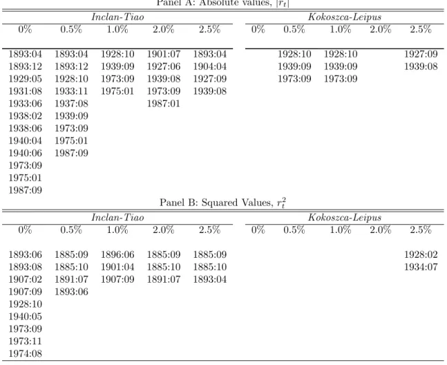
We compute the IT and KL tests on squared- and absolute-valued series. Although both transformations track the dynamics of the second-order moment, the information conveyed by those transformations is not necessarily the same, and as a result, the inferred number of breaks, and even their estimated location, may signi…cantly vary from using one proxy or the other; see Andreou and Ghysels (2002) and Cuñado et al. (2006). Since in‡uential outliers are expected to have a detrimental impact on the ability of the tests, we apply a trimming procedure to exclude the largest observations and check the robustness of any preliminary conclusion. Many papers in applied …nance control for outliers by …ltering top percentiles, observations that lie beyond some pre-determined level, or simply by removing speci…c observations, such as October 1987. Along with the non-trimming fraction (0%), we also apply conservative trimming fractions ranging from 0.5% (thus …ltering only 7 observations) to 2.5% (35 observations) to remove most extreme observations. If conclusions change dramatically after removing a few observations, then preliminary conclusions may be spurious and purely driven by outliers.

[Insert Table 2 about here]

The estimated break-locations are reported in Table 2. As expected from our previous analysis, the IT test tends to identify a relatively large number of breaks when applied on the original series, whereas the KL test tends to …nd signi…cantly smaller numbers. Similar evidence is observed, for instance, in Cuñado et al. (2006). More speci…cally, the IT test on absolute-valued (squared) returns …nds up to 12(9) breaks at a 5% nominal level, whereas the KL test cannot reject the null hypothesis in any of those series.6 _Likely

owing to the pervasive e¤ects of outliers, the IT test seems to identify short-lived structural breaks (e.g., 1940.04-1940.06), and outliers (e.g., the 1987 crash) as structural breaks. The KL test is unable to detect breaks around the GD.

The spuriousness of these results is evident after controlling for outliers, since the main conclusions dramatically change after …ltering just a small set of observations. It su¢ ces to remove the most in‡uential 0.5% to dramatically reduce the number of breaks found by the IT test (the IT test on _jrtj only …nds breaks around the beginning and end of the GD and the end of the 19th century) and to allow the KL test on _jrtj to detect the GD instability. This empirical exercise perfectly illustrates the main conclusions discussed theoretically and analytically in the previous sections.

5

Conclusions

In this paper, the size properties of CUSUM-type tests for detecting structural breaks in variance when the series of interest include some of the most relevant features that charac-terize …nancial data were analysed. Our special focus has been on additive outliers, which prove able to generate large size distortions in these tests. The most sensitive procedure is

6_{When applying the tests onjr}

tjandr2t with no previous …ltering, the …rst potential break dates found

are 1940:05 and 1940:06, respectively. In the case of the IT test, both dates are identi…ed as break-points, so that the ICSS algorithm continues. The KL test, on the other hand, fails to reject the null, and therefore the iterative procedure stops. These results remain valid even when using a 10% nominal level.

the one by Inclán and Tiao (1994), which should be applied with considerable caution on …nancial data. On the other hand, the procedure by Kokoszka and Leipus (2000) exhibits much better behaviour, at least under the conditions considered in this paper. In particu-lar, the asymptotic distribution of the test statistic is the standard one, and the estimator of the break point is consistent. However, in …nite-samples large size distortions due to the presence of outliers may be observed. As in the case of strongly-persistent volatility patterns, certain characteristics of the empirical data generating process in …nancial time series may cause major distortions in the small-sample performance of CUSUM-type tests. Consequently, a question of empirical relevance is what to do with extreme anom-alous observations. Bai (1998) proposed the use of robust procedures in the context of regressions with structural changes and additive outliers. In this spirit Fiteni (2004) has recently proposed the use of bounded-in‡uence estimators. These methods may outper-form least-squares based estimators under possible contaminated distributions, as they are speci…cally designed to be used even under arbitrarily large outliers. Since the stan-dard CUSUM test for detecting structural breaks in variance build on least-squares (or maximum likelihood) estimates , the use of bounded-in‡uence estimators may provide fur-ther improvements of the small-sample performance of this approach. The …ndings and general discussion in our paper support the empirical pursuit of this interesting question in future research.

A

Appendix

Proof of Lemma 3.1.

We consider = 0 in A1 for simplicity but without loss of generality. Let IT; =

P[T ]

t=1 [ t E( t)] and denote the j-th entry of this vector as Ij; . Under A2 and A4, the covariance matrix ofIT; ; ; is diagonal because theIj; terms are uncorrelated, and

I1; ; I4; and I5; satisfy a functional central limit theorem (FCLT) for mixing sequences (martingale di¤erences) under A3 (A3’), while I4; ; I5; and I6; verify directly the FCLT from Donsker’s lemma under A2, c.f. White (2000) and Deng and Perron (2008a). Hence,

1

p

TIj; )

p_!

jjW( );where !jj is the j-th element of the main diagonal in : It follows from the Gaussian properties of the Wiener process that p1

TIT; )

1=2_{W(r); where}

W(r) is a 6-dimensional Wiener process. Since r2

t = 10 t; with 1 a vector of ones in R6, and E(r_t2) = 10E( t); then P[T ] t=1 r 2 t E(rt2) = P6

j=1Ij; : The Cramer-Rao device completes the proof.

Proof of Lemma 3.2. Since p1 T P[T ] t=1 [~r 2 t E(rt2)] = p1_T P[T ]

t=1 10[ t E( t)] +op(1); it follows that the limit distribution of the functional converges weakly to the distribution of 10W( ) = W( ), a standard Wiener process, with scalar variance 10 _{1 =tr( ): This yields the required}

result. Part (ii) of the lemma is immediate for = 1, and part (iii) follows, similar to Lemma 3.1, from applying the weak law of large numbers; see White (2000).

Observe thatDT (k)can be rewritten asCT (T) 1 [CT (k) (k=T)CT (T)] = CT (T) 1 GT (k)+ op(1) where CT (k) = Pk_t=1rt2. Therefore, p1_TDT (k) = h CT(T) T i 1h 1 p TGT (k) i +op(1). From i) and ii) of Lemma 3.2 it follows that p1

T CT (k) k

T CT(T) )

p

M4W ( )

where from Lemma 3.2iii), CT(T)

T p

!V ar(rt) = 2"+p

2 ₊ 2 ₊ 2_{:From this result and} the continuos mapping theorem, it follows that

arg max 1 k T r T 2jDT (k)j ) M14=2 p 2 2 "+p 2_+p 2₊ 2 sup 2[0;1]j W ( )_j:

For the KL test, assume that_Mc4;T is a consistent estimator ofM4. Standard HAC-type estimators render this property under the set of assumptions discussed. From Lemma 3.2 and the continuous mapping theorem it follows straightforwardly that,

arg max1 k T jGT (k)j p T_Mc4;T = arg max1 k T CT (k) k T CT (T) p T_Mc4;T ) sup 2[0;1]j W ( )_j:

This completes the proof. Proof of Theorem 3.2.

Note that we can writebk= arg max1 k T k(T_T k) 1_kPk_t=1r2t 1 T k PT t=k+1r 2 t arg max1 k T jRk;Tj, whereRk;T is de…ned implicitly. Next, noteE(Rk;T) = (1 )1k k + (1 )1k>k ;

and E(Rk ;T) = (1 ), so jE(Rk ;T)j jE(Rk)j = j j( ) (1 )1k k +

j j ( )1k>k with1( ) being an indicator function. HencejE(Rk ;T)j jE(Rk)j

j j j jmin_f ;1 _g:Setting =_b;it can be shown that_{j j j bj}min_f ;1 _g

2 max 1 k TjRk;T E(Rk;T)j or, equivalently, jb j 1 Targ max1 k T 4Pk_t=1jr2 t E(r2t)j j jmin_f ;1 _g:

Next, denote k;T =T 1arg max1 k T Pk_t=1jrt2 E(r2t)j: For some >0; and Theorem 4.1 in Kokoszka and Leipus (2000), it follows that

Pr ( k;T > ) 2 2_T2 T 1 X t=0 v u u tV ar r2 t+1 t X i;j=1 Cov r2 i; r2j + 1 2_T2 T 1 X t=0 V ar r2_t+1 :

Under A2 and A4, Cov "2

i; "2j =O jt jj ; so Cov r2i; r2j has …nite upper bounds that decay exponentially. Also, Cov r2

i; rj2 = Cov "2i; "2j +V ar(Zi)1i=j + V ar( i)1i=j: For i = j; 0 Cov r2

i; r2j ; with C1 +V ar(Zi) +V ar( i) < 1; for some constant 0 < C₁ sup_tE("4_t); from Cauchy-Schwartz’s inequality. Note for i ₆= j,

Cov r2

i; r2j = Cov "2i; "2j and, therefore, 0 Cov ri2; rj2 C1 ji jj with 0 < 1 ruling the correlation pattern as a function of the speci…c model. Since0 Cov r2

i; r2j

ji jj _{uniformly for 1 i; j T; and denoting} 2

sup = max1<t<TV ar("2t); we have

Pr ( k;T > ) 2Kp1_T + 2 sup 2_T K2 2p_T; where K1 = 4 3 q 2

K2 > K1 >0: Finally, Pr (_{jb j}> ) Pr k;T > j j min_f ;1 _g 4 16K2 2 2_{(minf ;1 g)}2p_T = C 2 2p_T: This completes the proof.

References

[1] Aggarwal R, Inclán C, Leal R. 1999. Volatility in emerging stock markets. Journal

of Financial and Quantitative Analysis 34: 33-55.

[2] Andreou E, Ghysels E. 2002. Detecting multiple breaks dynamics.Journal of Applied

Econometrics 17: 579-600.

[3] Andreou E, Ghysels E. 2004. The impact of sampling frequency and volatility esti-mators and change-point test. Journal of Financial Econometrics 2: 290-318. [4] Bai J. 1998. Estimation of multiple-regime regressions with least absolutes deviation.

Journal of Statistical Planning 74: 103-134.

[5] Chen G, Choi Y, Zhou Z. 2005. Nonparametric estimation of structural change points in volatility models for time series.Journal of Econometrics 16: 79-114.

[6] Cuñado J, Gómez-Biscarri J, Pérez F. 2006. Changes in the dynamic behavior of emerging market volatility: Revisiting the e¤ects of …nancial liberalization.Emerging

Markets Review 7: 261-278.

[7] Deng A, Perron P. 2008a. The limit distribution of the Cusum of squares test under general mixing conditions.Econometric Theory 24: 809-822.

[8] Deng A, Perron P. 2008b. A non-local perspective on the power properties of the CUSUM and CUSUM of squares tests for structural change.Journal of Econometrics

142: 212-240.

[9] Franses PH, Haldrup H. 1994. The e¤ects of additive outliers on tests of unit Roots and cointegration. Journal of Business and Economic Statistics 12: 471-478.

[10] Fiteni I. 2004. -estimators of regression models with structural change of unknown location. Journal of Econometrics 119: 19-44.

[11] Inclán C, Tiao CJ. 1994. Use of cumulative sums of squares for retrospective detection of changes of variance. Journal of the American Statiscal Association 89: 913-923. [12] Kokoszka P, Leipus R. 2000. Change-point estimation in ARCH models. Bernoulli

[13] McConnell M, Perez-Quirós G. 2000. Output ‡uctuations in the United States: what has changed since the early 1980s? American Economic Review 90: 1464-76.

[14] Pagan AR, Schwert GW. 1990. Testing for covariance stationarity in stock market data. Economics Letters 33, 165-170.

[15] Sensier M, and van Dijk D. 2004. Testing for volatility changes in US macroeconomic time series, Review of Economics and Statistics 86: 833-839.

[16] van Dijk D, Franses PH, Lucas A. 1999. Testing for ARCH in the presence of additive outliers.Journal of Applied Econometrics 14: 539-562.

[17] Vogelsang T. 1999. Two simple procedures for testing for a unit root when there are additive outliers. Journal of Time Series Analysis 20: 237–52.

A

Figures

Figure 1. Empirical size of the Inclán-Tiao test (5% nominal size) with

outlier-contaminated data. 0 0.1 0.2 0.3 0.4 0.5 0 2 4 6 0 0.2 0.4 0.6 0.8 p IT test,_δ =1 λ E m pi ri c al s iz e, 5% nom inal

Note: The DGP isrt = t+Dt[ + vt]; t; vt iidN (0;1),Dt=f 1;0gwith

probabili-ties_fp=2;1 p_g:The results are based on 15,000 simulations forT = 1000and = 1. The test statistic is compared to the critical values from SSBB under the null of variance homogeneity. The experimental proportion of rejections are displayed on the vertical axis.

Figure 2. Empirical size of the Kokoszka-Leipus test (5% nominal size) with outlier-contaminated data. 0 0.1 0.2 0.3 0.4 0.5 0 2 4 6 0.025 0.03 0.035 0.04 0.045 0.05 p KL test,δ =1 λ E m pi ri c al s iz e, 5% nom inal

Note: The DGP is rt = t+Dt[ + vt]; t; vt iidN (0;1), Dt = f 1;0g with

proba-bilities _fp=2;1 p_g: The long-run variance ofr2

t E(rt2)is computed using the Newey-West

estimator with Bartlett kernel and bandwidth h =

h

4 (100=T)2=9

i

: The results are based on 15,000 simulations forT = 1000and = 1. The test statistic is compared to the critical values from SSBB under the null of variance homogeneity. The experimental proportion of rejections are displayed on the vertical axis.

Figure 3. Empirical size of the Inclán-Tiao test (5% nominal size) with GARCH

[GARCH2] errors and outliers.

0 0.1 0.2 0.3 0.4 0.5 ₀ 1 2 3 4 5 0 0.2 0.4 0.6 0.8 1 λ IT test,δ =1 p E m pi ri c al s iz e, 5% nom inal

Note: See caption under Figure 1, but considering in this case that the conditional volatility 2_t follows a GARCH(1,1) process with parameters( ; ) = (0:1;0:8):

Figure 4. Empirical size of the Kokoszka-Leipus test (5% nominal size) with GARCH errors [GARCH1] and outliers.

0 0.1 0.2 0.3 0.4 0.5 0 1 2 3 4 5 0.04 0.045 0.05 0.055 0.06 0.065 λ KL test,δ =1 p E m pi ri c al s iz e, 5% nom inal

Note: See caption under Figure 2, but considering in this case that the conditional volatility 2_t follows a GARCH(1,1) process with parameters( ; ) = (0:1;0:5):

Figure 5. Empirical size of the Kokoszka-Leipus test (5% nominal size) with GARCH

errors [GARCH2] and outliers.

0 0.1 0.2 0.3 0.4 0 1 2 3 4 5 0 0.1 0.2 0.3 0.4 λ KL test,δ =1 p E m pi ri c al s iz e, 5% nom inal

Note: See caption under Figure 2, but considering in this case that the conditional volatility 2_t follows a GARCH(1,1) process with parameters( ; ) = (0:1;0:8):

A

T

a

b

le

s

T A B L E 1 . A v er a g e es ti m a ti o n ( E ( b )) a n d st a n d a rd er ro r (s .e . x 1 0 0 ) o f b b a se d o n r 2 :t ii d GA R CH1 G AR CH2 0.2 5 0 .50 0.75 0 .25 0.50 0. 75 0.25 0. 50 0.75 ( ; p ) E ( b ) s.e. E ( b ) s.e. E ( b ) s.e. E ( b ) s.e. E ( b ) s.e. E ( b ) s.e. E ( b ) s.e. E ( b ) s.e. E ( b ) s.e. (0 ; 0) 0.2 89 0.05 0.50 9 0. 02 0. 745 0.02 0.30 6 0. 07 0. 514 0.03 0.742 0.0 3 0. 358 0 .12 0.530 0.06 0.7 28 0. 08 (0 ; 0 ; 10) 0.2 93 0.06 0.50 9 0. 02 0. 743 0.03 0.30 9 0. 08 0. 515 0.03 0.740 0.0 4 0. 361 0 .12 0.530 0.06 0.7 28 0. 08 (0 ; 0 : 25) 0.2 97 0.07 0.51 0 0. 02 0. 739 0.04 0.31 2 0. 08 0. 515 0.03 0.736 0.0 4 0. 362 0 .13 0.530 0.06 0.7 24 0. 09 (0 ; 0 : 50) 0.3 04 0.08 0.51 2 0. 03 0. 734 0.04 0.31 9 0. 09 0. 519 0.04 0.733 0.0 5 0. 367 0 .13 0.530 0.06 0.7 20 0. 09 (1 ; 0) 0.2 89 0.05 0.50 9 0. 02 0. 745 0.02 0.30 7 0. 07 0. 514 0.03 0.742 0.0 3 0. 358 0 .12 0.530 0.05 0.7 30 0. 08 (1 ; 0 ; 10) 0.2 97 0.06 0.50 1 0. 02 0. 739 0.03 0.31 4 0. 08 0. 515 0.03 0.736 0.0 4 0. 361 0 .12 0.530 0.06 0.7 23 0. 09 (1 ; 0 : 25) 0.3 06 0.08 0.51 0 0. 03 0. 734 0.05 0.32 2 0. 09 0. 516 0.04 0.729 0.0 6 0. 367 0 .13 0.530 0.06 0.7 17 0. 10 (1 ; 0 : 50) 0.3 20 0.10 0.51 3 0. 04 0. 721 0.07 0.33 3 0. 11 0. 518 0.05 0.719 0.0 8 0. 375 0 .14 0.532 0.07 0.7 07 0. 11 (2 : 5 ; 0) 0.2 89 0.05 0.50 9 0. 02 0. 746 0.02 0.30 7 0. 08 0. 514 0.03 0.742 0.0 3 0. 357 0 .12 0.528 0.06 0.7 29 0. 08 (2 : 5 ; 0 ; 10) 0.3 20 0.10 0.51 0 0. 05 0. 714 0.08 0.33 3 0. 11 0. 515 0.05 0.710 0.0 9 0. 378 0 .14 0.531 0.08 0.7 01 0. 12 (2 : 5 ; 0 : 25) 0.3 51 0.14 0.51 4 0. 08 0. 683 0.12 0.36 7 0. 14 0. 517 0.08 0.682 0.1 3 0. 394 0 .16 0.529 0.10 0.6 70 0. 15 (2 : 5 ; 0 : 50) 0.3 91 0.17 0.51 8 0. 11 0. 655 0.16 0.39 6 0. 17 0. 524 0.11 0.656 0.1 6 0. 420 0 .17 0.536 0.12 0.6 47 0. 18 (5 ; 0) 0.2 89 0.06 0.50 9 0. 02 0. 746 0.02 0.30 7 0. 08 0. 514 0.03 0.742 0.0 3 0. 358 0 .12 0.530 0.06 0.7 29 0. 08 (5 ; 0 ; 10) 0.4 12 0.19 0.50 6 0. 14 0. 603 0.19 0.41 5 0. 19 0. 509 0.14 0.604 0.1 9 0. 431 0 .19 0.519 0.15 0.6 01 0. 20 (5 ; 0 : 25) 0.4 55 0.20 0.51 4 0. 17 0. 566 0.21 0.45 9 0. 20 0. 513 0.17 0.569 0.2 1 0. 465 0 .20 0.522 0.18 0.5 67 0. 21 (5 ; 0 : 50) 0.4 77 0.21 0.52 3 0. 18 0. 556 0.22 0.48 5 0. 21 0. 523 0.19 0.561 0.2 2 0. 488 0 .21 0.526 0.19 0.5 56 0. 22 Not e: Av erage v alue of the b re ak -f rac ti on estimato r b and stand a rd er ror (x100) , with b = k = T ; and bk: ma x1 k T P k t=1 r 2 t k = T P T t=1 r 2 t . The DG P is rt = t t + Bt [ + vt ] , with t ;v t iid N (0 ; 1) ; Bt = f 1 ; 1 ; 0 g with probab iliti es f p= 2 ;p= 2 ; 1 p g : F or t < [ T ] ; E ( t t ) = 1 and E ( t t ) = 1 : 5 otherwise. Th e v olati lit y pro cess t fo llo ws a n ii d se q u en ce, an d a GAR CH( 1,1) mo de l w ith para m eters ( ; ) = (0 : 1 ; 0 : 5) [G AR CH1], and ( ; ) = (0 : 1 ; 0 : 8) [G AR CH2].

TABLE 2. Testing for multiple change-points in the volatility of monthly US market index returns.

Panel A: Absolute values,_jrtj

Inclan-Tiao Kokoszca-Leipus 0% 0.5% 1.0% 2.0% 2.5% 0% 0.5% 1.0% 2.0% 2.5% 1893:04 1893:04 1928:10 1901:07 1893:04 1928:10 1928:10 1927:09 1893:12 1893:12 1939:09 1927:06 1904:04 1939:09 1939:09 1939:08 1929:05 1928:10 1973:09 1939:08 1927:09 1973:09 1973:09 1931:08 1933:11 1975:01 1973:09 1939:08 1933:06 1937:08 1987:01 1938:02 1939:09 1938:06 1973:09 1940:04 1975:01 1940:06 1987:09 1973:09 1975:01 1987:09

Panel B: Squared Values,r2t

Inclan-Tiao Kokoszca-Leipus 0% 0.5% 1.0% 2.0% 2.5% 0% 0.5% 1.0% 2.0% 2.5% 1893:06 1885:09 1896:06 1885:09 1885:09 1928:02 1893:08 1885:10 1901:04 1885:10 1885:10 1934:07 1907:02 1891:07 1907:09 1891:07 1893:04 1907:09 1893:06 1928:10 1940:05 1973:09 1973:11 1974:08

Note: The date of the break is estimated under the IT and KL test procedures at the 5% nominal signi…cance level and given the trimming fractions presented in the columns (0%, 0.5%, 1.0%, 2.0%, 2.5%). For instance, 0.5% indicates that the tests are applied after removal of the 0.5% most extreme observations in the sample.

WORKING PAPERS 2008

1/08 THE DETERMINANTS OF PORTUGUESE BANKS’ CAPITAL BUFFERS — Miguel Boucinha

2/08 DO RESERVATION WAGES REALLY DECLINE? SOME INTERNATIONAL EVIDENCE ON THE DETERMINANTS OF RESERVATION WAGES

— John T. Addison, Mário Centeno, Pedro Portugal

3/08 UNEMPLOYMENT BENEFITS AND RESERVATION WAGES: KEY ELASTICITIES FROM A STRIPPED-DOWN JOB SEARCH APPROACH

— John T. Addison, Mário Centeno, Pedro Portugal

4/08 THE EFFECTS OF LOW-COST COUNTRIES ON PORTUGUESE MANUFACTURING IMPORT PRICES — Fátima Cardoso, Paulo Soares Esteves

5/08 WHAT IS BEHIND THE RECENT EVOLUTION OF PORTUGUESE TERMS OF TRADE? — Fátima Cardoso, Paulo Soares Esteves

6/08 EVALUATING JOB SEARCH PROGRAMS FOR OLD AND YOUNG INDIVIDUALS: HETEROGENEOUS IMPACT ON UNEMPLOYMENT DURATION

— Luis Centeno, Mário Centeno, Álvaro A. Novo

7/08 FORECASTING USING TARGETED DIFFUSION INDEXES — Francisco Dias, Maximiano Pinheiro, António Rua

8/08 STATISTICAL ARBITRAGE WITH DEFAULT AND COLLATERAL — José Fajardo, Ana Lacerda

9/08 DETERMINING THE NUMBER OF FACTORS IN APPROXIMATE FACTOR MODELS WITH GLOBAL AND GROUP-SPECIFIC FACTORS

— Francisco Dias, Maximiano Pinheiro, António Rua

10/08 VERTICAL SPECIALIZATION ACROSS THE WORLD: A RELATIVE MEASURE — João Amador, Sónia Cabral

11/08 INTERNATIONAL FRAGMENTATION OF PRODUCTION IN THE PORTUGUESE ECONOMY: WHAT DO DIFFERENT MEASURES TELL US?

— João Amador, Sónia Cabral

12/08 IMPACT OF THE RECENT REFORM OF THE PORTUGUESE PUBLIC EMPLOYEES’ PENSION SYSTEM — Maria Manuel Campos, Manuel Coutinho Pereira

13/08 EMPIRICAL EVIDENCE ON THE BEHAVIOR AND STABILIZING ROLE OF FISCAL AND MONETARY POLICIES IN THE US

— Manuel Coutinho Pereira

14/08 IMPACT ON WELFARE OF COUNTRY HETEROGENEITY IN A CURRENCY UNION — Carla Soares

15/08 WAGE AND PRICE DYNAMICS IN PORTUGAL — Carlos Robalo Marques

16/08 IMPROVING COMPETITION IN THE NON-TRADABLE GOODS AND LABOUR MARKETS: THE PORTUGUESE CASE — Vanda Almeida, Gabriela Castro, Ricardo Mourinho Félix

17/08 PRODUCT AND DESTINATION MIX IN EXPORT MARKETS — João Amador, Luca David Opromolla

18/08 FORECASTING INVESTMENT: A FISHING CONTEST USING SURVEY DATA — José Ramos Maria, Sara Serra

19/08 APPROXIMATING AND FORECASTING MACROECONOMIC SIGNALS IN REAL-TIME — João Valle e Azevedo

20/08 A THEORY OF ENTRY AND EXIT INTO EXPORTS MARKETS — Alfonso A. Irarrazabal, Luca David Opromolla

21/08 ON THE UNCERTAINTY AND RISKS OF MACROECONOMIC FORECASTS: COMBINING JUDGEMENTS WITH SAMPLE AND MODEL INFORMATION

— Maximiano Pinheiro, Paulo Soares Esteves

22/08 ANALYSIS OF THE PREDICTORS OF DEFAULT FOR PORTUGUESE FIRMS — Ana I. Lacerda, Russ A. Moro

23/08 INFLATION EXPECTATIONS IN THE EURO AREA: ARE CONSUMERS RATIONAL? — Francisco Dias, Cláudia Duarte, António Rua

2009

1/09 AN ASSESSMENT OF COMPETITION IN THE PORTUGUESE BANKING SYSTEM IN THE 1991-2004 PERIOD — Miguel Boucinha, Nuno Ribeiro

2/09 FINITE SAMPLE PERFORMANCE OF FREQUENCY AND TIME DOMAIN TESTS FOR SEASONAL FRACTIONAL INTEGRATION

— Paulo M. M. Rodrigues, Antonio Rubia, João Valle e Azevedo

3/09 THE MONETARY TRANSMISSION MECHANISM FOR A SMALL OPEN ECONOMY IN A MONETARY UNION — Bernardino Adão

4/09 INTERNATIONAL COMOVEMENT OF STOCK MARKET RETURNS: A WAVELET ANALYSIS — António Rua, Luís C. Nunes

5/09 THE INTEREST RATE PASS-THROUGH OF THE PORTUGUESE BANKING SYSTEM: CHARACTERIZATION AND DETERMINANTS

— Paula Antão

6/09 ELUSIVE COUNTER-CYCLICALITY AND DELIBERATE OPPORTUNISM? FISCAL POLICY FROM PLANS TO FINAL OUTCOMES

— Álvaro M. Pina

7/09 LOCAL IDENTIFICATION IN DSGE MODELS — Nikolay Iskrev

8/09 CREDIT RISK AND CAPITAL REQUIREMENTS FOR THE PORTUGUESE BANKING SYSTEM — Paula Antão, Ana Lacerda

9/09 A SIMPLE FEASIBLE ALTERNATIVE PROCEDURE TO ESTIMATE MODELS WITH HIGH-DIMENSIONAL FIXED EFFECTS

— Paulo Guimarães, Pedro Portugal

10/09 REAL WAGES AND THE BUSINESS CYCLE: ACCOUNTING FOR WORKER AND FIRM HETEROGENEITY — Anabela Carneiro, Paulo Guimarães, Pedro Portugal

11/09 DOUBLE COVERAGE AND DEMAND FOR HEALTH CARE: EVIDENCE FROM QUANTILE REGRESSION — Sara Moreira, Pedro Pita Barros

12/09 THE NUMBER OF BANK RELATIONSHIPS, BORROWING COSTS AND BANK COMPETITION — Diana Bonfi m, Qinglei Dai, Francesco Franco

13/09 DYNAMIC FACTOR MODELS WITH JAGGED EDGE PANEL DATA: TAKING ON BOARD THE DYNAMICS OF THE IDIOSYNCRATIC COMPONENTS

— Maximiano Pinheiro, António Rua, Francisco Dias

14/09 BAYESIAN ESTIMATION OF A DSGE MODEL FOR THE PORTUGUESE ECONOMY — Vanda Almeida

15/09 THE DYNAMIC EFFECTS OF SHOCKS TO WAGES AND PRICES IN THE UNITED STATES AND THE EURO AREA — Rita Duarte, Carlos Robalo Marques

16/09 MONEY IS AN EXPERIENCE GOOD: COMPETITION AND TRUST IN THE PRIVATE PROVISION OF MONEY — Ramon Marimon, Juan Pablo Nicolini, Pedro Teles

17/09 MONETARY POLICY AND THE FINANCING OF FIRMS — Fiorella De Fiore, Pedro Teles, Oreste Tristani

18/09 HOW ARE FIRMS’ WAGES AND PRICES LINKED: SURVEY EVIDENCE IN EUROPE

— Martine Druant, Silvia Fabiani, Gabor Kezdi, Ana Lamo, Fernando Martins, Roberto Sabbatini

19/09 THE FLEXIBLE FOURIER FORM AND LOCAL GLS DE-TRENDED UNIT ROOT TESTS — Paulo M. M. Rodrigues, A. M. Robert Taylor

20/09 ON LM-TYPE TESTS FOR SEASONAL UNIT ROOTS IN THE PRESENCE OF A BREAK IN TREND — Luis C. Nunes, Paulo M. M. Rodrigues

21/09 A NEW MEASURE OF FISCAL SHOCKS BASED ON BUDGET FORECASTS AND ITS IMPLICATIONS — Manuel Coutinho Pereira

22/09 AN ASSESSMENT OF PORTUGUESE BANKS’ COSTS AND EFFICIENCY — Miguel Boucinha, Nuno Ribeiro, Thomas Weyman-Jones

23/09 ADDING VALUE TO BANK BRANCH PERFORMANCE EVALUATION USING COGNITIVE MAPS AND MCDA: A CASE STUDY

— Fernando A. F. Ferreira, Sérgio P. Santos, Paulo M. M. Rodrigues

24/09 THE CROSS SECTIONAL DYNAMICS OF HETEROGENOUS TRADE MODELS — Alfonso Irarrazabal, Luca David Opromolla

25/09 ARE ATM/POS DATA RELEVANT WHEN NOWCASTING PRIVATE CONSUMPTION? — Paulo Soares Esteves

26/09 BACK TO BASICS: DATA REVISIONS — Fatima Cardoso, Claudia Duarte

27/09 EVIDENCE FROM SURVEYS OF PRICE-SETTING MANAGERS: POLICY LESSONS AND DIRECTIONS FOR ONGOING RESEARCH

— Vítor Gaspar , Andrew Levin, Fernando Martins, Frank Smets

2010

1/10 MEASURING COMOVEMENT IN THE TIME-FREQUENCY SPACE — António Rua

2/10 EXPORTS, IMPORTS AND WAGES: EVIDENCE FROM MATCHED FIRM-WORKER-PRODUCT PANELS — Pedro S. Martins, Luca David Opromolla

3/10 NONSTATIONARY EXTREMES AND THE US BUSINESS CYCLE — Miguel de Carvalho, K. Feridun Turkman, António Rua

4/10 EXPECTATIONS-DRIVEN CYCLES IN THE HOUSING MARKET — Luisa Lambertini, Caterina Mendicino, Maria Teresa Punzi

5/10 COUNTERFACTUAL ANALYSIS OF BANK MERGERS

— Pedro P. Barros, Diana Bonfi m, Moshe Kim, Nuno C. Martins

6/10 THE EAGLE. A MODEL FOR POLICY ANALYSIS OF MACROECONOMIC INTERDEPENDENCE IN THE EURO AREA — S. Gomes, P. Jacquinot, M. Pisani

7/10 A WAVELET APPROACH FOR FACTOR-AUGMENTED FORECASTING — António Rua

8/10 EXTREMAL DEPENDENCE IN INTERNATIONAL OUTPUT GROWTH: TALES FROM THE TAILS — Miguel de Carvalho, António Rua

9/10 TRACKING THE US BUSINESS CYCLE WITH A SINGULAR SPECTRUM ANALYSIS — Miguel de Carvalho, Paulo C. Rodrigues, António Rua

10/10 A MULTIPLE CRITERIA FRAMEWORK TO EVALUATE BANK BRANCH POTENTIAL ATTRACTIVENESS — Fernando A. F. Ferreira, Ronald W. Spahr, Sérgio P. Santos, Paulo M. M. Rodrigues

11/10 THE EFFECTS OF ADDITIVE OUTLIERS AND MEASUREMENT ERRORS WHEN TESTING FOR STRUCTURAL BREAKS IN VARIANCE