Cloud Computing and Software Services: Theory and Technique
John Doe
Contents
1 Transparent Cross-Platform Access to Software Services Using GridSolve
and GridRPC 1
1.1 Introduction to RPC and Network Based Software Services . . . 2
1.2 The GridRPC API . . . 3
1.3 GridSolve: A GridRPC Implementation . . . 7
1.3.1 Overview and Architecture . . . 8
1.3.2 Transparency and Ease of Use . . . 9
1.3.3 Scheduling in GridSolve . . . 11
1.4 RPC Transparency Issues . . . 17
1.5 Summary . . . 22
Chapter 1
Transparent Cross-Platform Access to
Software Services Using GridSolve
and GridRPC
Keith Seymour
1, Asim YarKhan
1, and Jack Dongarra
1 2Distributed computing can be daunting even for experienced programmers. Although many projects have been created to facilitate developing distributed applications, they are often quite complex in themselves. While many scientific applications could benefit from distributed computing, the complexity of the programming models can be a high barrier to entry, especially since many of these applications are developed by domain scientists without extensive training in software development. Thus, we believe that the paramount design consideration of a distributed computing model should be ease of use. With this in mind, we will discuss GridRPC, which is a model for remote procedure call in the context of a computational Grid or other loosely coupled distributed computing environment. Then we will discuss GridSolve, an implementation of the GridRPC model.
1Department of Electrical Engineering and Computer Science, University of Tennessee, Knoxville, TN 37919 USA 2Computer Science and Mathematics Division, Oak Ridge National Laboratory, Oak Ridge, TN 37831 USA
1.1
Introduction to RPC and Network Based Software Services
RPC (Remote Procedure Call) refers to a mechanism that allows invoking a procedure on a remote machine as if the procedure was implemented locally. The invocation is typically carried out by means of a communications library and “stub” procedures . The library handles packing up the user’s data, sending it across the network to the remote machine, and unpacking it there. The process of packing the data into a standard format (especially important for cross-platform scenarios) is referred to asdata marshalling. Once the data has been transferred, the RPC system invokes the user’s procedure and passes the data to it. From that point, the user’s procedure takes control and executes until completion. Then the process is reversed to send the results back to the client machine. The “stub” procedures are used to enable linking the programs (since the actual procedure does not exist locally to be linked) and to initiate the RPC process via calls to the RPC library. This standard RPC process is depicted in Figure 1.1.
One of the earliest implementations of RPC was part of the Cedar project at Xerox Palo Alto Research Center [1], although the concept had been discussed for several years prior to the Xerox implementation [2]. Cedar used RPC to enable distributed computing primarily because of the ease-of-use inherent in the RPC paradigm. Procedure calls were considered a well-understood mechanism and provided clean and simple semantics. Around that time, RPC was also being investigated in the context of distributed operating systems. In a critique of RPC as a general communications model for arbitrary applications [3], it is argued (among other things) that since true transparency is impossible, it may be better to design a partially transparent mechanism. If the system is transparent to the point that the programmers really do not know if their calls will be executed locally or remotely, then there could be serious performance implications (e.g. if a sorting routine called a comparison procedure thousands of times unaware that it would be executed remotely). Most modern RPC-like systems are not aiming for that level of transparency, but the critique raises issues that are still relevant today. In this chapter, we will touch on these and other RPC transparency issues in the context of a Grid-based RPC implementation.
high-1.2. THE GRIDRPC API 3 performance computing is efficiency. If the user’s local machine is slow, but remote resources are fast, RPC can provide an overall reduction in execution time, even including the cost of data marshalling. However, traditional RPC only allows for synchronous calls. That is, once the procedure is invoked, the client program must sit idle until it completes, even if it had other useful computations it could be doing. The synchronous model also prevents submitting multiple parallel RPC requests, which could provide for even better overall per-formance. Another limitation of the traditional RPC model is that the mapping of RPC request to server is very simplistic, often requiring the use of a specific machine. Intelligent selection of servers could drastically improve the performance. Also the use of client-side stubs requires language-specific generators for all client language bindings. Furthermore, consider the implications of this compilation requirement on interactive computing environ-ments like Matlab or Octave. In those cases, the user cannot be expected to compile stubs just to make use of a remote procedure.
RPC remains a useful mechanism due to its elegance and simplicity, but the aforemen-tioned limitations have prompted several extensions to the model, including asynchronous calls, task parallel calls, real-time resource scheduling, fault tolerance, security, and stubless operation. We will be discussing GridRPC, a recent specification of an API for Grid-based RPC, as well as a complete implementation of this API within the GridSolve system.
1.2
The GridRPC API
As mentioned in the previous section, the difficulty of using most programming models is a hindrance to the widespread adoption of grid computing. One particular programming model that has proven to be viable is an RPC mechanism tailored for the grid, or “GridRPC”. Although at a very high level view the programming model provided by GridRPC is that of standard RPC plus asynchronous coarse-grained parallel tasking, in practice there are a variety of features that will largely hide the dynamicity, insecurity, and instability of the grid from the programmers. As such, GridRPC allows not only enabling individual applications to be distributed, but also can serve as the basis for even higher-level software substrates
such as distributed, scientific components on the grid.
The GridRPC API [4] represents ongoing work to standardize and implement a portable and simple remote procedure call mechanism for grid computing. This standardization effort is being pursued through the Open Grid Forum (previously Global Grid Forum) Research Group on Advanced Programming Models [5].
In this section, we informally describe the GridRPC model and the functions that comprise the API. A detailed listing of the GridRPC function prototypes can be found in the GridSolve Users’ Guide [6].
Function Handles and Session IDs Two fundamental objects in the GridRPC model are function handles and session IDs. The function handle represents a mapping from a function name to an instance of that function on a particular server. The GridRPC API does not dictate the mechanics of resource discovery since different underlying GridRPC implementations may use vastly different protocols. Once a particular function-to-server mapping has been established by initializing a function handle, all RPC calls using that function handle will be executed on the server specified in that binding. A session ID is an identifier representing a particular non-blocking RPC call. The session ID is used throughout the API to allow users to obtain the status of a previously submitted non-blocking call, to wait for a call to complete, to cancel a call, or to check the error code of a call.
Initializing and Finalizing Functions The initialize and finalize functions are similar to the MPI initialize and finalize calls. Client GridRPC calls before initialization or after finalization will fail.
• grpc initialize reads the configuration file and initializes the required modules. • grpc finalize releases any resources being used by GridRPC.
Remote Function Handle Management Functions Thefunction handle management
1.2. THE GRIDRPC API 5
• grpc function handle defaultcreates a new function handle using the default server.
This could be a pre-determined server name or it could be a server that is dynamically chosen by the resource discovery mechanisms of the underlying GridRPC implementa-tion, such as the GridSolve agent.
• grpc function handle init creates a new function handle with a server explicitly
specified by the user.
• grpc function handle destruct releases the memory associated with the specified
function handle.
• grpc get handle returns the function handle corresponding to the given session ID
(that is, corresponding to that particular non-blocking request).
GridRPC Call Functions A GridRPC may be either blocking (synchronous) or non-blocking (asynchronous) and it accepts a variable number of arguments (like printf) de-pending on the calling sequence of the particular routine being called.
• grpc callmakes a blocking remote procedure call with a variable number of arguments. • grpc call async makes a non-blocking remote procedure call with a variable number
of arguments.
Asynchronous GridRPC Control Functions The following functions apply only to previously submitted non-blocking requests.
• grpc probechecks whether the asynchronous GridRPC call has completed.
• grpc probe orchecks whether any of the previously issued non-blocking calls in a given
set have completed.
• grpc cancel cancels the specified asynchronous GridRPC call. • grpc cancel all cancels allpreviously issued calls.
Asynchronous GridRPC Wait Functions The following five functions apply only to previously submitted non-blocking requests. These calls allow an application to express de-sired non-deterministic completion semantics to the underlying system, rather than repeat-edly polling on a set of sessions IDs. (From an implementation standpoint, such information could be conveyed to the OS scheduler to reduce cycles wasted on polling.)
• grpc wait blocks until the specified non-blocking requests to complete.
• grpc wait andblocks until allof the specified non-blocking requests in a given set have
completed.
• grpc wait orblocks until any of the specified non-blocking requests in a given set has
completed.
• grpc wait allblocks untilallpreviously issued non-blocking requests have completed.
• grpc wait anyblocks until any previously issued non-blocking request has completed.
Error Reporting Functions Of course it is possible that some GridRPC calls can fail, so we need to provide the ability to check the error code of previously submitted requests. The following error reporting functions provide error codes and human-readable error de-scriptions.
• grpc error string returns the error description string, given a numeric error code. • grpc get error returns the error code associated with a given non-blocking request. • grpc get failed sessionid returns the session ID of the last invoked GridRPC call
that caused a failure.
Related Work on Network Enabled Servers Several Network Enabled Servers (NES) provide mechanisms for transparent access to remote resources and software. Ninf-G [7] is an implementation of the GridRPC API that can function on top of a variety of Grid middleware environments such as Globus, Condor and SSH (as of version 5). Ninf-G provides an interface
1.3. GRIDSOLVE: A GRIDRPC IMPLEMENTATION 7 definition language that allows services to be easily added, and client APIs are provided in C and Java. Security, scheduling and resource management are generally left up to the underlying middleware.
The DIET (Distributed Interactive Engineering Toolbox) project [8] is a client-agent-server RPC architecture which uses the GridRPC API as its primary interface. A CORBA Naming Service handles the resource registration and lookup, and a hierarchy of agents handles the scheduling of services on the resources. An API is provided for generating service profiles and adding new services, and a C client API exists.
NEOS [9] is a network-enabled problem-solving environment designed as a generic appli-cation service provider (ASP). Any appliappli-cation that can be changed to read its inputs from files, and write its output to a single file can be integrated into NEOS. The NEOS Server acts as an intermediary for all communication. The client data files go to the NEOS server, which sends the data to the solver resources, collects the results and then returns the results to the client. Clients can use email, web, sockets based tools and CORBA interfaces.
Other projects are related to various aspects of GridSolve. For example, task farming style computation is provided by the Apples Parameter Sweep Template (APST) project [10], the Condor Master Worker (MW) project [11], and the Nimrod-G project [12]. Request sequencing and workflow management is handled by projects like Condor DAGman [13].
1.3
GridSolve: A GridRPC Implementation
GridSolve is a GridRPC-compliant distributed computing system that provides an efficient and easy-to-use programming model for using remote computational resources. Remote resources can provide access to specialized hardware or highly tuned software with the per-formance and features desired by a computational scientist. The basic goal of GridSolve is to provide a easy to use, uniform, portable and efficient way to access computational resources over a network.
1.3.1 Overview and Architecture
The GridSolve system is comprised of a set of loosely connected machines. By loosely con-nected, we mean that these machines are on the same local, wide or global area network, and may be administrated by different institutions and organizations. Moreover, the GridSolve system is able to support these interactions in a heterogeneous environment, i.e. machines of different architectures, operating systems and internal data representations can participate in the system at the same time.
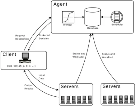
Figure 1.2 shows the global conceptual picture of the GridSolve system. In this figure, we can see the three major components of the system: the client, theagent, and theservers
(computational or software resources). GridSolve and systems like it are often referred to as Grid Middleware. GridSolve acts as a glue layer that brings the application or user together with the hardware and/or software needed to complete useful tasks. At the top tier, the GridSolve client library is linked in with the user’s application. The application then makes calls to GridSolve’s application programming interface (GridRPC) for specific services. Through the GridRPC API, GridSolve client-users gain access to aggregate resources without needing to know anything about distributed computing or maintaining software libraries . In fact, the user does not even have to know remote resources are involved. The GridSolve agent maintains a database of GridSolve servers along with their capabilities (hardware performance and allocated software) and dynamic usage statistics. It uses this information to allocate server resources for client requests. The agent finds servers that will service requests the quickest, balances the load amongst its servers and keeps track of failed ones. The GridSolve server is a daemon process that awaits client requests. The server can run on single workstations, clusters of workstations, symmetric multi-processors or machines with massively parallel processors. A key component of the GridSolve server is a source code generator which parses a GridSolve Interface Definition Language (gsIDL) file. This gsIDL file contains information that allows the GridSolve system to create new service modules and incorporate new functionalities. In essence, the gsIDL defines a interface and wrapper that GridSolve uses to call functions being incorporated. The (hidden) semantics of a GridSolve request are:
1.3. GRIDSOLVE: A GRIDRPC IMPLEMENTATION 9 1. Client contacts the agent with a service request description
2. Agent returns a brokered decision containing a list of capable servers 3. Client contacts server and sends input data
4. Server receives the data and runs appropriate service
5. Client receives the output results or error status from the server
From the user’s perspective, the call to GridSolve acts very much like the call to the original function. The GridSolve calls can also be made in an asynchronous fashion, so that the client can either perform other tasks during the RPC call, or the client can submit multiple parallel RPC service requests and then probe for their completion.
1.3.2 Transparency and Ease of Use
In addition to the standard GridRPC API, GridSolve provides a number of features that make it easier to use and provide a substantial benefit. These features are intended to make it easier for the service provider to add services, and easier for the user to take advantage of these services.
Stubless Clients GridSolve is designed so that the clients do not require client-side stubs to be generated and compiled in order to call remote procedures. This is in contrast with many other RPC systems, where a client-stub needs to be generated and bound for each remote function. Several dynamically reconfigurable languages such as Java and Python allow clients to incorporate new functionality on-the-fly, but traditional languages such as C and Fortran cannot easily do so. GridSolve accomplishes this by using generalized mar-shalling routines on the client and the server. Using a stubless client in GridSolve enables it to make new server functionality available to its clients without requiring any changes at the client-side. The drawback of this approach is that type checking cannot be done at the time of calling the GridSolve API. However, this stubless approach fits well with the goal of
making GridSolve easy to use. After a client is deployed, no additional changes are required for client to access new functions deployed at any server.
Scientific Computing Environments GridSolve has a strong focus on ease-of-use, since this is still perceived to be a substantial barrier to the general adoption of distributed and grid computing services. As such, in addition to C and Fortran client interfaces, GridSolve provides client bindings to several high-level SCEs (scientific computing environments) such as Matlab, Octave and IDL (Interactive Data Language). In this way it becomes possible to combine high-performance distributed grid resources with the flexibility, familiarity and productivity of SCEs. The SCE bindings allow the user to make calls to remote functions in a natural way, and the GridSolve client handles all the details of converting data from the SCEs internal representations to GridSolve data representations. Then the GridSolve client submits the RPC request to the GridSolve server, and when the remote reply is received, the client converts it back to the natural format for the SCE. This smooth integration with SCEs is one of the most successful features of GridSolve.
Server Administration We have implemented a simple technique for adding arbitrary services to a running server. First, the new service should be built as a library or object file. Then the user writes a specification of the service parameters in a gsIDL (GridSolve Interface Definition Language) file. The GridSolve service compiler processes the gsIDL and generates a wrapper which is automatically compiled and linked with the service library or object files. The services are compiled as external executables with interfaces to the server described in a standard format. The server re-examines its own configuration and installed services periodically to detect new services. In this way it becomes aware of the additional services without re-compilation or restarting of the server itself.
Server administrators may specify arbitraryserver attributesin a configuration file. These attributes are used to enable filtering or criteria matching in the selection of resources. For example, the server could have attributes describing the machine’s architecture or amount of memory. These attributes are sent to the agent and stored in its database so that clients can make complex requests (e.g. only give me x86 servers with more than 2 GB of memory).
1.3. GRIDSOLVE: A GRIDRPC IMPLEMENTATION 11 The agent can very quickly filter service requests using these attributes to find matches with the appropriate servers.
Server administrators can also add restrictions in the configuration file. This allows restricting access to the server under certain conditions, such as during peak times or when there are already a certain number of jobs already running.
1.3.3 Scheduling in GridSolve
Scheduling is essential for achieving an efficient and responsive distributed system. In a distributed, heterogeneous environment like the Grid, services can achieve very different performance depending on many factors, including the network conditions, the server speeds, the temporary load on the server, and the efficiency of installed software. These factors need to be accounted for when scheduling service requests onto servers. GridSolve has several alternative scheduling methods available, and the topic of scheduling remain a active research area within GridSolve.
Agent Scheduling In agent based scheduling, the agent uses knowledge of the requested service, information about the parameters of the service request from the client, and the current state of the resources to score the possible servers and return the servers in sorted order.
When a service is started, the server informs the agent about services that it provides and the computational complexity of those services. This complexity is expressed using two integer constants a and b and is evaluated as aNb, where N is the problem size. At
startup, the server notifies the agent about its computational speed (approximate MFlops from a simple benchmark) and it continually updates the agent with information about its workload. When an agent receives a request for a service with a particular problem size, it uses the service complexity and the server status information to estimate the time to completion on each server providing that service. It orders the servers in terms of time to completion, and then returns the list of servers to the client. The client then sends the
service request to the fastest server. If that fails for some reason, the client can resubmit the service request to the next fastest service, thus providing a basic level of fault tolerance. This scheduling heuristic, summarized in Figure 1.3 is known as Minimum Completion Time. It is simple to implement and works well in many practical cases. Each service request should be assigned to the server that would complete the service in the minimum time, assuming that the currently known loads on the servers will remain constant during the execution and the communication costs between the client and all the servers are the same.
However, the Minimum Completion Time heuristic does not try to maximize the through-put when servers are allowed to run multiple services and there are many more requested services than available servers. Since an estimate of the execution time for currently execut-ing service is available, this knowledge could be used to schedule new service requests more intelligently. Some explorations of alternative scheduling heuristics using historical execution trace information in are described in [14].
Server Performance Prediction The server also plays an important role in helping the agent-based scheduling to work effectively. To efficiently schedule an application requires being able to accurately predict the duration of the requests that compose the application. However, predicting the duration of a request is a difficult task. Indeed, the duration might depend on the data (size and values), on the machine where the application is run, and on the implementation of the service. Even when the duration of a service does not depend on the data values (as is the case with many linear algebra kernels), predicting this duration is hard. In GridSolve, the duration of the task is described in the gsIDL (GridSolve Interface Description Language) file using the highest degree of the complexity polynomial, which gives an approximation of the number of operations the service has to perform when the inputs are known. The server’s speed (number of operations per second) is computed by running a simple benchmark when the server is launched. The server periodically updates its current workload, which is used by the agent to scale down the server’s speed. Then the estimated duration of the task is computed at run-time by dividing the estimated number of operations by the current speed of the server. However, computing the duration of a service based on the complexity polynomial has several drawbacks.
1.3. GRIDSOLVE: A GRIDRPC IMPLEMENTATION 13 First, even though the complexity polynomial does not depend on the implementation, different implementations of the same algorithm do not necessarily have the same speed. Assume for instance that the service is the matrix multiply routine of the BLAS (Basic Linear Algebra Subroutines). There are a lot of different implementations of the same BLAS API, ranging from reference BLAS (a non-optimized Fortran version), to automatically tuned libraries such as ATLAS [15] and up to specific implementations optimized for a precise version of a certain CPU such as the goto BLAS) [16]. The complexity of these implementations is always the same (O(N3) for multiplying matrices of order N), but the
execution time might be completely different (for instance the reference BLAS are about 6 times slower than the vendor optimized version on some CPUs). This effect is not taken into account by the standard Minimum Completion Time scheduling heuristic in GridSolve.
Moreover, obtaining the speed of the machine with a benchmark assumes that the flop-rate of each service is the same as the benchmark. In practice this is not true because compute-intensive services achieve higher flop rates than data-compute-intensive services. In GridSolve, the server’s speed is estimated by running a Linpack benchmark, which performs close to the peak flop rate of the processor. This is appropriate when the requested service is a compute-intensive one such as for a linear algebra kernel. However, if the service is I/O bound (such as database access) or memory constrained (such as an out-of-core computation), the estimated runtime is likely to be a huge underestimation of the actual runtime.
Finally, for a given service a slight change of a parameter may lead to a different algorithm and a different time to execute the service. For instance the matrix-matrix multiply routine of the BLAS (dgemm) performs C ←αAB+βC, where A, B and C are matrices. It is easy
to see that the case α = 1, β = 0 is completely different from the case α = 0 and β = 1. However, in the current GridSolve model, since the values of α and β are not related to the size of data they do not appear in the complexity model for the dgemm service.
To solve the problems described above, we propose using a complexity template model for each service that is instantiated on each server for each different use case of the service. This template model consists of a polynomial of the parameters of the problem and a set of category variables. The polynomial describes the behavior of the service and has coefficients
that will be assigned by GridSolve based on the prior execution performance history. The use of categories differentiates the separate performance classes which cannot be modeled as a continuous complexity function.
GridSolve uses a parametric regression system to compute or update the coefficients for the complexity templates at runtime. Each time the server runs the service it updates the coefficients of the model using this run and the previous ones. A certain number of previous runs are stored on the server’s local disk, which can be reused if the server has to be stopped and restarted. The server periodically sends updates of the coefficients to the agent, which evaluates the expressions at runtime to get an accurate prediction of the execution time of the service. The detailed complexity parameters that the agent receives from the server allow more accurate scheduling decisions to be made.
Scheduling using Proxies for Computational Resources In this server based ap-proach to scheduling, GridSolve creates server-proxies to delegate the scheduling to special-ized scheduling and execution services such as batch systems, Condor or LFC (LAPACK for Clusters). The GridSolve agent sees the server-proxy as a single server entity, even though the server-proxy can represent a large number of actual resources, and so the proxy handles the scheduling for these resources rather than the GridSolve agent.
The GridSolve agent can decide to assign the service request to a server-proxy based on several factors (e.g., the proxy can register itself with the agent as a virtual server with a large amount of processing power). The server-proxy will delegate the request to the specialized service (e.g. Condor), which schedules and executes the request. The server-proxy then returns the results back to the client.
Client Scheduling Scheduling based purely on computation cost may give poor results because the communication cost can be a very large factor in the overall RPC cost, especially in a WAN environment. While choosing the fastest server may minimize the execution time, if that server is on a distant network, the communication cost can easily overshadow the savings in execution time.
1.3. GRIDSOLVE: A GRIDRPC IMPLEMENTATION 15 To eliminate this weakness, we need an estimate of the network performance between the client and the servers that could possibly execute the service. This can be difficult to know ahead of time given the dynamic nature of the system, so we gather the information empirically at the time the call is made. When the client gets a list of servers from the agent, it is sorted based only on the estimate of the computational cost. Normally the client would simply submit the service request to the first server on the list, but instead we first measure the bandwidth from the client to the top few servers using a simple 32 KB ping-bong benchmark. Given the total data size and the network speed, we compute an estimate of the total communication and computation RPC time for the servers and reorder the list of servers.
There is some cost associated with performing these measurements, but our expectation is that the reduction in total RPC time will compensate for the overhead. Nevertheless, we try to keep the measurement overhead to a minimum. The time required to do the mea-surement will depend on the number of servers which have the requested problem and the bandwidth and latency from the client to those servers. When the data size is relatively small, the measurements are not performed because it would take less time to send the data than it would take to do the measurements. Also, since a given service may be available on many servers, the cost of measuring the network speed to all of them could be prohibitive. Therefore, the number of servers to be measured is limited to those with the highest com-putational performance. The exact number of measurements is configurable by the client. Once the measurements have been made, they can be cached for a certain amount of time so that subsequent calls on that client do not have to repeat the same measurement. The lifetime of the cached measurements is configurable by the user.
There are many other projects that monitor grid performance, see [17] or [18] for a review. For example, the Network Weather Service (NWS) [19], is a popular general system service that can monitor the performance of network bandwidth and latency (as well as other measures) and provide a statistical forecast for future performance. However, for the GridSolve system, most of the existing systems are inappropriate because clients enter and leave GridSolve dynamically, making it difficult to measure and retain the communication costs between the clients and the full set of servers. Moreover, NWS is required to be
configured on each end, which necessitates some expertise that we do not assume. Hence, we have chosen to implement low overhead probes as a way of building up the communication cost matrix between a client and the servers relevant to that client.
Task Graph Scheduling There are two deficiencies associated with the standard RPC-based model when a computational problem essentially forms a workflow consisting of a sequence of tasks, among which there exist data dependencies. First, intermediate results are passed among tasks by first returning to the client, resulting in additional data transport between the client and the servers, which is pure overhead. Second, since the execution of each individual task is a separate RPC session, it is difficult to explore the potential paral-lelism among tasks where there is no immediate data dependency. Our previous approach to request sequencing partially solves the problem of unnecessary data transport by clustering a sequence of tasks based upon the dependency among them and scheduling them to run collectively. This approach has two limitations. First, the only mode of execution it supports is on a single server. Second, it prevents the potential parallelism among tasks from being explored. Recent work on GridSolve has focused on creating an enhanced request sequenc-ing technique that eliminates those limitations and solves the above problems. The core features of this work include direct inter-server data transfer and the capability of parallel task execution. The objective of this work is to simplify the parallel execution of data-driven workflow applications in GridSolve.
In GridSolve request sequencing, a request is defined as a single GridRPC call to an avail-able GridSolve service. A data-driven workflow application is constructed as a sequence of requests, among which there may exist data dependencies. For each workflow application, the sequence of requests is scanned, and the data dependency between the requests is an-alyzed. The output of the analysis is a DAG representing the workflow: tasks within the workflow are represented as nodes, and data dependencies among tasks are represented as edges. The workflow scheduler then schedules the DAG to run on the available servers. A set of tasks can potentially be executed concurrently if their dependencies permit it.
In order to eliminate unnecessary data transport when tasks are run on multiple servers, the standard RPC-based computational model of GridSolve has been extended to support
1.4. RPC TRANSPARENCY ISSUES 17 direct data transfer among servers. Specifically, in order to avoid the case that intermediate results are passed among tasks via the client, servers must be able to pass intermediate results among each other, without the client being involved.
Recent experiments [20] demonstrated promising benefit from eliminating unnecessary data transfer and exploiting the parallelism found by automatically constructing and an-alyzing the task graph. The algorithm for workflow scheduling and execution currently used in GridSolve request sequencing is primitive in that it does not take into consideration the differences among tasks and does not consider the overall mutual impact between task clustering and network communication. We are planning to substitute a more advanced algorithm for this primitive one. Additionally, we are currently working on providing sup-port for advanced workflow patterns such as conditional branches and loops, which are not supported in the current implementation.
1.4
RPC Transparency Issues
As we mentioned in the introduction, there are some non-trivial issues to deal with when aiming for a transparent RPC implementation. In this section, we discuss some of these issues within the context of the GridRPC specification and our GridSolve implementation.
Parameter Passing In local procedure calls, arguments are passed by value or by refer-ence. Pass-by-value means that the actual value of the argument is passed to the procedure (e.g. ifxhas the value 5 andxis passed by value, then the procedure is given the value 5). In contrast, pass-by-reference means that a pointer is passed to the procedure, which must be dereferenced to obtain the actual values (e.g. if the value pointed to byxis stored in memory address 0x100, then the procedure is given the value 0x100). Pass-by-reference is useful in a couple of scenarios. First, it allows the procedure to modify the value of an argument, which is not possible in a pass-by-value situation. Also, it is more efficient for passing large data structures like matrices because only one address needs to be passed instead of all the values.
In the context of RPC, the problem with pass-by-reference is that the remote machine is in a different address space, so any pointers from the client machine will be meaningless. This could be handled by making requests back to the client when data from the remote pointer is accessed, but that would be very inefficient. The typical approach (and the one implemented in GridSolve) is to pass a copy of the data referenced by the pointer and then restore any modifications to the data upon completion of the RPC. However, in an asynchronous situation, the user needs to be careful because any modifications to the referenced data made after the call but before the results from the RPC are restored would be lost.
Another complication with parameter passing in RPC is that of complex or user-defined data structures. Sun RPC uses XDR (External Data Representation) [21], which is a stan-dard for describing and encoding arbitrary data. In GridSolve, we chose to avoid XDR for performance reasons and because almost all of the procedures we were dealing with used simple data structures like vectors and matrices. There are tradeoffs between transparency, flexibility, simplicity, and efficiency. We gave up some transparency and flexibility to gain simplicity and efficiency.
Binding to Servers RPC binding refers to locating the remote host with the procedure to be invoked and then finding the correct server process on that host. Traditional RPC required specifying the remote host name explicitly. When the user is expected to supply the host names for the remote calls, the veneer of transparency begins to erode. Also, it becomes more than just a transparency issue when asynchronous RPC is considered. In that case, the selection of the remote host to satisfy the request can have a big effect on the performance.
The GridRPC function handle represents a mapping from a service descriptor (in this case a simple character string) to the remote server that will be used to execute the func-tion. This mapping could be specified by the user or determined by the middleware using simple resource discovery mechanisms or possibly some more sophisticated scheduling algo-rithms. In the end, the GridRPC specification leaves the issue of binding up to the various implementations.
1.4. RPC TRANSPARENCY ISSUES 19 The normal GridRPC calling sequence is to first initialize the handle and bind to a server using a call togrpc function handle default() followed by a call togrpc call()(or one of its brethren) at some point later. In the case of the GridSolve implementation, there is a slight problem with performing the scheduling in this scenario. GridSolve relies on having access to the values of the arguments ingrpc call()at the time the scheduling is performed so it can estimate the execution time and communication cost of sending the data. However, at the time grpc function handle default() is called, we do not know which values will be used in the eventual call, so scheduling is not possible.
To deal with this issue, we allow the user to specify a special host name when initializing the function handle. The special name signifies to the GridSolve internals that the function handle binding should be delayed until the first time the handle is used to make a call. Subsequent calls using that function handle will not change the binding, so the semantics of successive GridRPC calls is not altered.
In terms of transparency, GridSolve does require the user to know the host name of the GridSolve Agent, which performs the binding and scheduling, but the user never needs to know any of the server details. This seems like a reasonable tradeoff because of multiple benefits provided by the agent.
Exception Handling and Fault Tolerance Whenever communication with remote ma-chines is involved, there is the possibility for new and subtle errors to appear. This can destroy the sense of transparency because now the user must deal with many new failure scenarios that would never happen with a local procedure call. The GridRPC specifica-tion largely avoids attempting to maintain this kind of procedure-level transparency. The GridRPC calls have their own return values and error codes that must be dealt with ap-propriately. Any errors from the remote procedure itself must be passed back as an output argument of the RPC.
Despite the lack of transparency in exception handling, the GridRPC specification leaves open the possibility of implementing transparent fault tolerance. In GridSolve, if a call fails the system will automatically find another server to resubmit the job to. This is completely
transparent, so the user never knows that there were failures in the system. This brings up several issues of how to detect failures. There are many failure scenarios and the handling of each one is a bit different, but these implementation details do not really affect the user’s perception of RPC transparency. The issue of fault tolerance also affects the issue of binding, since when errors occur the final server handling the request might be different from the one originally selected. GridSolve allows the user to enable or disable the fault tolerant mode in order to match the desired GridRPC semantics.
Data Representation The internal representation of data is an important issue in RPC because the local and remote machines may have different word lengths, floating-point for-mats, and byte orderings. If the user has to think about their data representation or data structures, the illusion of transparency is lost. We mentioned XDR earlier as a solution to the issue of passing complex data structures, but XDR also handles conversion of primitive data types between architectures by using a common intermediate representation. The GridRPC specification says nothing about data conversion, so it is left up to the implementors to decide. In GridSolve we implemented a receiver makes rightprotocol which allows the client to send data in its native format which the receiver then converts to its own native format if needed. This avoids having to do two separate conversions (each end converting between native and common representations) as well as avoiding making an extra copy of the data on the sending side. GridSolve is still limited in its support for complex data structures, but we feel the increased efficiency in the common cases is worth making the tradeoff.
Performance While we go to great effort to ensure good performance in GridSolve, the fact remains that extra communication overhead is inherent in any RPC. It was mentioned in [3] that if you had a truly transparent RPC for arbitrary applications, serious performance degradation could be inadvertently introduced. Of course, GridRPC specifies a different API for remote calls, so users will be aware of which calls are local and which are remote. Nevertheless, to achieve the best performance in an RPC-based application, the developers should carefully consider the ratio of computation time to communication time (since proces-sor power has been increasing faster than communication speed, this issue gets more serious
1.4. RPC TRANSPARENCY ISSUES 21 every year). Take matrix multiplication as an example. We compute C ←αAB+βC where
A, B, and C are matrices. For the sake of simplicity, assume they are all square matrices of size N ×N. The communication costs will be on the order of:
Cinput = 3× N2×elementsize bandwidth Coutput = N2×elementsize bandwidth Ctotal = Cinput+Coutput
Where elementsize is the size of each matrix element in bytes andbandwidthis the number of bytes per second for the network. Assuming a local network bandwidth of 11 MByte/s and an element size of 8 bytes, the communication cost for N = 3000 is around 25 seconds. The computational costs will be on the order of:
P = (2 3N
3)/M
p
Where Mp is the performance of the machine in floating point operations per second. At
N = 3000 and local machine performance of Mp = 800 Mflop/s, the local computation cost
would be roughly 22.5 seconds. So, it costs more to send the data (not counting remote execution time) than it would to just do the computation locally. Since the computation cost is growing faster than the communication cost, there will eventually be a crossover point where it makes sense to do the RPC, but it depends on the performance of the remote machine relative to the local machine as well as the network speed (WANs are often much worse than our 11 MByte/s LAN example).
While this example might be discouraging, there are still many favorable scenarios for RPC especially when taking into account task parallelism. One example is in parameter sweep problems, where the data being distributed is relatively small, and many servers can be used asynchronously and simultaneously to evaluate different input data with the output being collated in some way. Tasks that are suited to RPC computation include Evolutionary Algorithms (genetic algorithms, etc.) and Monte Carlo style algorithms and optimization algorithms.
Security Unlike with local procedures, when executing a remote procedure the data is exposed on the network and therefore susceptible to snooping. Security is another area that is not addressed by the GridRPC specification, but the various implementations choose their own strategies. We have not implemented any data encryption methods in GridSolve. It is an important issue, but most of our users are running the entire GridSolve infrastructure on their local networks (e.g. behind firewalls). Because of that, there has not been a huge demand for encryption in GridSolve, but it should be straightforward to add since we have already implemented a transparent data compression module, and encryption could be added to that module at the data transport level.
Transparency Trying to achieve total transparency (if it is even possible) would result in unexpected behavior and unacceptable performance degradation. As it was mentioned earlier, from a design standpoint total transparency might not be the ideal anyway. We have attempted to design a system that is transparent in the sense of shielding users from unnecessary details and allowing for relatively painless conversion of code to a distributed implementation. The user still retains control over their application in deciding which func-tions are appropriate for remote processing. But the user does not need to know which server will be used, how the data will be converted, whether the job was resubmitted to another server due to failures, etc. This level of partial transparency allows the GridSolve system to provide better overall performance for the users while leaving the user in control of their application.
1.5
Summary
Using distributed grid resources in an simple and effective manner is difficult, though there are multiple programming models that are attempting to meet this challenge. The GridRPC API is a simple and portable programming model providing a standardized mechanism for accessing grid resources. GridSolve provides an implementation of GridRPC and adds a substantial list of features that are designed to make access to grid resources transparent and easier to accomplish. Client bindings for commonly used Scientific Computing Environments
1.5. SUMMARY 23 (e.g., Matlab, Octave, IDL) make it easy for a computational scientist to use grid resources from within their preferred tools. Transparent scheduling via the GridSolve agent relieves the user from having to know the details of the servers and service providers. Service level fault tolerance provides a simple and usable mode for failure recovery. Task graph scheduling allows the composition of sequences of tasks into a inferred workflow, without requiring additional input from the user. Using all these techniques and more, GridSolve has been working to make the grid easier to use, and further research on this goal continues.
References
[1] Andrew D. Birrell and Bruce Jay Nelson. Implementing Remote Procedure Calls. ACM Transactions on Computer Systems, pages 39–59, 1984.
[2] J. E. White. A High-level Framework for Network-based Resource Sharing. In Proceed-ings of the National Computer Conference, June 1976.
[3] A. S. Tanenbaum and R. van Renesse. A Critique of the Remote Procedure Call Paradigm. InProceedings of the EUTECO 88 Conference, pages 775–783, 1988.
[4] K. Seymour, N. Hakada, S. Matsuoka, J. Dongarra, C. Lee, and H. Casanova. Overview of GridRPC: A Remote Procedure Call API for Grid Computing. In M. Parashar, editor,GRID 2002, pages 274–278, 2002.
[5] Global Grid Forum Research Group on Programming Models. http://www.gridforum.org/7 APM/APS.htm.
[6] J. Dongarra, Y. Li, K. Seymour, and A. YarKhan. Users’ Guide to GridSolve V0.19. In-novative Computing Laboratory. Technical Report, University of Tennessee, Knoxville, TN, June 2008.
[7] Y. Tanaka, H. Nakada, S. Sekiguchi, Suzumura Suzumura, and S. Matsuoka. Ninf-G: A reference implementation of RPC-based programming middleware for Grid computing.
Journal of Grid Computing, 1(1):41–51, 2003.
[8] E. Caron, F. Desprez, F. Lombard, J.-M. Nicod, L. Philippe, M. Quinson, and F. Suter. A Scalable Approach to Network Enabled Servers (Research Note). Lecture Notes in Computer Science, 2400, 2002.
Optimiza-tion: Version 4 and Beyond. Technical Report ANL/MCS-P947-0202, Mathematics and Computer Science Division, Argonne National Laboratory, Argonne, IL, February 2002. [10] Henri Casanova, Graziano Obertelli, Berman Berman, and Rich Wolski. The AppLeS Parameter Sweep Template: User-Level Middleware for the Grid. In Proceedings of Supercomputing’2000 (CD-ROM), Dallas, TX, Nov 2000. IEEE and ACM SIGARCH. [11] Jeff Linderoth, Sanjeev Kulkarni, Jean-Pierre Goux, and Michael Yoder. An Enabling
Framework for Master-Worker Applications on the Computational Grid. InProceedings of the Ninth IEEE Symposium on High Performance Distributed Computing (HPDC9), pages 43–50, Pittsburgh, PA, August 2000.
[12] David Abramson, Rajkumar Buyya, and Jonathan Giddy. A Computational Economy for Grid Computing and its Implementation in the Nimrod-G Resource Broker. Future Generation Computer Systems, 18(8):1061–1074, October 2002.
[13] James Frey, Todd Tannenbaum, Ian Foster, Miron Livny, and Steve Tuecke. Condor-G: A computation management agent for multi-institutional grids. Cluster Computing, 5:237–246, 2002.
[14] Yves Caniou and Emmanuel Jeannot. Experimental study of multi-criteria scheduling heuristics for GridRPC systems. InACM-IFIP Euro-Par 2004, Pisa, Italy, Sept 2004. [15] R. Clint Whaley and Jack J. Dongarra. Automatically Tuned Linear Algebra Software
(ATLAS). In ACM, editor,SC’98: High Performance Networking and Computing: Pro-ceedings of the 1998 ACM/IEEE SC98 Conference: Orange County Convention Center, Orlando, Florida, USA, November 7–13, 1998, New York, NY 10036, USA and 1109 Spring Street, Suite 300, Silver Spring, MD 20910, USA, 1998. ACM Press and IEEE Computer Society Press. Best Paper Award for Systems.
[16] Kazushige Goto and Robert van de Geijn. High-Performance Implementation of the Level-3 BLAS. Technical Report CS-TR-06-23, The University of Texas at Austin, Department of Computer Sciences, May 5 2006. Thu, 4 Jan 107 17:59:12 GMT.
[17] Dong Lu, Yi Qiao, Peter A. Dinda, and Fabi´an E. Bustamante. Characterizing and Predicting TCP Throughput on the Wide Area Network. In 25th International Con-ference on Distributed Computing Systems (ICDCS 2005), 6-10 June 2005, Columbus, OH, USA, pages 414–424, 2005.
1.5. SUMMARY 25
Future Generation Computer Systems, 21(1):163–188, January 2005.
[19] Rich Wolski, Neil T. Spring, and Jim Hayes. The Network Weather Service: A Dis-tributed Resource Performance Forecasting Service for Metacomputing. Future Gener-ation Computer Systems, 15(5–6):757–768, 1999.
[20] Y. Li, J. Dongarra, K. Seymour, and A. YarKhan. Request Sequencing: Enabling Workflow for Efficient Problem Solving in GridSolve. In International Conference on Grid and Cooperative Computing (GCC 2008), Oct 2008.
[21] Sun Microsystems Inc. XDR: External Data Representation Standard. RFC 1014, Sun Microsystems, Inc., Jun 1987.
Client Application RPC Stub RPC Library Operating System RPC Stub RPC Library Operating System Remote Procedure
Client Machine Server Machine
N e t w o r k
Figure 1.1: Client-server interaction in standard RPC
A g e n t Monitor Database Scheduler Client grpc_call(&h, a, b, c, ...); Request Description Brokered Decision Servers Servers I n p u t D a t a O u t p u t Results Status and Workload Status and Workload
Figure 1.2: GridSolve architecture showing interactions between client, agent and servers
for all servers Si that can provide the desired service
T1(Si) = estimated amount of time for computation on Si
T2(Si) = estimated time for communicating input and output data
T(Si) = T1(Si) +T2(Si) estimated total time using Si
select the server Sm which has the minimum time, where T(Sm) = min T(Si)∀i