RUHR
ECONOMIC PAPERS
Gold Price Forecasts in a Dynamic
Model Averaging Framework – Have the
Determinants Changed Over Time?
Dirk G. Baur
Joscha Beckmann
Robert Czudaj
Imprint
Ruhr Economic Papers
Published by
Ruhr-Universität Bochum (RUB), Department of Economics Universitätsstr. 150, 44801 Bochum, Germany
Technische Universität Dortmund, Department of Economic and Social Sciences Vogelpothsweg 87, 44227 Dortmund, Germany
Universität Duisburg-Essen, Department of Economics Universitätsstr. 12, 45117 Essen, Germany
Rheinisch-Westfälisches Institut für Wirtschaftsforschung (RWI) Hohenzollernstr. 1-3, 45128 Essen, Germany
Editors
Prof. Dr. Thomas K. Bauer
RUB, Department of Economics, Empirical Economics Phone: +49 (0) 234/3 22 83 41, e-mail: [email protected] Prof. Dr. Wolfgang Leininger
Technische Universität Dortmund, Department of Economic and Social Sciences Economics – Microeconomics
Phone: +49 (0) 231/7 55-3297, e-mail: [email protected] Prof. Dr. Volker Clausen
University of Duisburg-Essen, Department of Economics International Economics
Phone: +49 (0) 201/1 83 -3655, e-mail: [email protected] Prof. Dr. Roland Döhrn, Prof. Dr. Manuel Frondel, Prof. Dr. Jochen Kluve RWI, Phone: +49 (0) 201/81 49 -213, e-mail: [email protected]
Editorial Offi ce
Sabine Weiler
RWI, Phone: +49 (0) 201/81 49 -213, e-mail: [email protected]
Ruhr Economic Papers #506
Responsible Editor: Volker Clausen
All rights reserved. Bochum, Dortmund, Duisburg, Essen, Germany, 2014 ISSN 1864-4872 (online) – ISBN 978-3-86788-581-2
The working papers published in the Series constitute work in progress circulated to stimulate discussion and critical comments. Views expressed represent exclusively the
Ruhr Economic Papers #506
Dirk G. Baur, Joscha Beckmann, and Robert Czudaj
Gold Price Forecasts in a Dynamic
Model Averaging Framework – Have the
Bibliografi sche Informationen
der Deutschen Nationalbibliothek
Die Deutsche Bibliothek verzeichnet diese Publikation in der deutschen National-bibliografi e; detaillierte National-bibliografi sche Daten sind im Internet über:
http://dnb.d-nb.de abrufb ar.
http://dx.doi.org/10.4419/86788581 ISSN 1864-4872 (online)
Dirk G. Baur, Joscha Beckmann, and Robert Czudaj
1Gold Price Forecasts in a Dynamic
Model Averaging Framework – Have the
Determinants Changed Over Time?
Abstract
The price of gold is infl uenced by a wide range of local and global factors such as commodity prices, interest rates, infl ation expectations, exchange rate changes and stock market volatility among others. Hence, forecasting the price of gold is a notoriously diffi cult task and the main problem a researcher faces is to select the relevant regressors at each point in time. This combination of model and parameter uncertainty is explicitly accounted for by Dynamic Model Averaging which allows both the forecasting model and the coeffi cients to change over time. Based on this framework, we systematically evaluate a large set of possible gold price determinants and use both the predictive likelihood and the mean squared error as a measure of the forecasting performance. We carefully assess which predictors are relevant for forecasting at diff erent points in time through the posterior probability. Our fi ndings show that (1) DMA improves forecasts compared to other frameworks and (2) provides clear evidence for the time-variation of gold price predictors.
JEL Classifi cation: C32, G10, G15, F37
Keywords: Bayesian econometrics; dynamic model averaging; forecasting; gold September 2014
1Dirk G. Baur, Kuehne Logistics University, Hamburg; Joscha Beckmann, UDE and Kiel Institute for the World Economy; Robert Czudaj, UDE. – Thanks for valuable comments are due to the participants of the 12th INFINITI Conference on International Finance, Prato/Italy, the 10th BMRC-DEMS Conference on Macro and Financial Economics/Econometrics, London/UK, and the rotating lecture of the Ruhr Graduate School in Economics, Essen/ Germany. – All correspondence to: Robert Czudaj, University of Duisburg-Essen, Department of Economics, Chair for Econometrics, 45117 Essen, Germany, e-mail: [email protected]
1
Introduction
There is now a large and growing academic literature on the financial economics of gold. Most studies focus on one of the key properties of gold, e.g. the inflation hedge property of gold (e.g. Blose, 2010, Jastram, 2009, and Beckmann and Czudaj, 2013), the currency hedge property of gold (e.g. Capie et al., 2005 and Sjaastadt and Scacciavillani, 1996) or the safe haven property of gold (e.g. Baur and Lucey, 2010) but do not entertain gold price forecasts.1 Interestingly, there is no established forecasting model for gold prices and no framework that simultaneously considers and evaluates all potential factors and their dynamics. This paper aims to fill this significant gap in the literature by adopting the Dynamic Model Averaging approach which is well-suited for forecasting under conditions of uncertainty. The question whether potential determinants of the gold price are also useful in a time-varying forecasting framework is of great interest for a broad audience. A significant in-sample, i.e. contemporaneous and thus non-predictive, relationship between the gold prices and particular determinants over a specific period does not provide a guarantee for success in terms of out-of-sample predictability. Hence, evaluating the evolution of gold price forecasts based on our framework offers an interesting perspective for researchers and market participants.
Overall, a researcher who aims at forecasting gold prices faces a variety of issues: Firstly, the deter-minants of gold potentially change over time resulting in model uncertainty, i.e. the set of variables that determine the price of gold varies. This can be illustrated by studying the dynamics of the gold price over the last decades: Having mostly fluctuated around a constant value in the 1980s and 1990s, the rapid increase observed in the 2000s might be attributed to variables which were not considered as important determinants up to that point in time. The task is further complicated by the fact that determinants might be important throughout the sample but to a different degree, resulting in pa-rameter uncertainty. It is, for example, well established, that the impact of stock market movements on gold varies over time and is generally higher during times of turbulence. Inflation or inflation
1Baker and Van Tassel (1985) and Pierdzioch et al. (2014) are notable exceptions. The latter also try to
account for model and parameter uncertainty, however they only consider six different predictors and apply model selection and aggregation methods that are based on recursive and rolling-window OLS estimates. The selection of the “optimal” forecast model and the weighting of several forecast models solely depend on the in-sample fit based on information criteria. The aspect which makes our forecasts superior compared to simple selection and aggregation methods is that our model weights are based on the forecasting performance of the models in previous periods.
expectations may also be relevant only at certain periods of time, e.g. when inflation expectations exceed a specific threshold. In summary, a researcher faces both uncertainty about the variables to include in a forecasting model - model uncertainty - and uncertainty about the time-variation of the parameters - parameter uncertainty. Raftery (1995) describes a common approach to account for model uncertainty by first fitting the full model, screen the t-statistics for the parameters, remove the variables for which these are small and then re-estimate the resulting, reduced, model. Raftery (1995) argues that researchers often proceed using the selected model as if it were the only model that had ever been considered. By choosing among a large number of models one increases the likelihood of finding significant variables by chance alone.2
An intuitive solution to avoid this model uncertainty is the combination of different models. An ad-hoc approach is to use a simple average of different forecasts. More sophisticated frameworks rely on Bayesian techniques, explicitly accounting for a large degree of uncertainty by assigning probabilities to each model conditional on previous forecasting performance. However, due to the need of determining a transition matrix Bayesian inference can suffer from a computational burden if many regressors are included. This becomes obvious ifmregressors are considered resulting in 2m possible model combinations. In other words, a forecasting model withm= 14 variables results in 16,384 model combinations. If the forecasting model is allowed to change at each point in timetthe number of combinations of models which must be estimated is even much higher.
Against this background, we adopt the Dynamic Model Averaging (DMA) approach introduced by Raftery et al. (2010) and applied by Koop and Korobilis (2012) for forecasting inflation. Such a framework has the advantage that both the forecasting model and the coefficients in each model are allowed to change over time. Another advantage is that a direct comparison with forecasts based on the “best” model at a certain point in time according to Dynamic Model Selection (DMS) can be drawn. From an economic point of view, the importance of each predictor over time can be analyzed by disentangling the dynamics of all underlying models simultaneously. A key ingredient is that a model will have more weight at timetif it has forecasted well in the period prior tot. In other words, sequential learning is a key part of the forecasting procedure.
Our main contribution is manifold. We analyze whether forecasts based on Dynamic Model Averaging
are able to systematically outperform the random walk for forecasting the price of gold. We also address the important question whether more parsimonious models should be preferred for forecasting. Finally, we systematically analyze the importance of different gold price predictors over time. In doing so, we examine how the weights attached to regressors evolve over time and whether model averaging or model selection provides superior results in terms of the forecasting performance. We consider Bayesian and classical criteria to assess the adequacy of the obtained forecast.
This paper is structured as follows: Section 2 presents the Dynamic Model Averaging framework. Section 3 introduces the data used in the estimation. Section 5 describes and discusses the estimation results and Section 6 summarizes the main findings and provides concluding remarks.
2
Methodology
In our forecasting setup we considerK different models,M1, . . . , MK, which are given by different subsets of possible predictorsxt= (xtj:j= 1, . . . , m),3and we allow for the uncertainty which model is the best at each point in timet. We apply a state space model which comprises anobservationand astate equationgiven by
yt=xt(k)θt(k)+ε(tk), (1)
θt(k)=θt(−k)1+δt(k), (2)
whereyt denotes the endogenous variable (i.e. the price of gold) andθ(tk)is a vector of regression parameters fork= 1, . . . , K. The measurement noiseεt(k)is distributed asN(0, Vt(k)) and the process noiseδt(k)asN(0, Wt(k)). Both the state vectorθ(tk)as well as the predictor vectorx(tk)are different for each model and the quantities belonging toMkare represented by the superscript (k). Fork= 1 Eq. (1) and (2) can be referred to as a standard state space model, which can be estimated adaptively with standard Kalman filtering.4
If the process is governed by modelMkat timet, thenLt=k. The evolution of the model changes can be determined by aK×Ktransition probability matrixP, wherepk,=P[Lt=|Lt−1=k] denotes
3xtincludes the timet−hinformation set and also includes an intercept. This means thatxtcontains the
predictors observed att−1, when using a forecast horizon ofh= 1.
its elements. SinceK = 2m, the dimension of this matrix depends on the number of predictorsm and unlessmis very small,P will be an enormous matrix. Hence, inference will be imprecise and the computation will take much time (Koop and Korobilis, 2012). Therefore, we avoid these problems by the use of an approximation proposed by Raftery et al. (2010) that includes a forgetting factor. This will be illustrated further below.
In our model setup the underlying state is characterized by the pair (Θt, Lt), where Θt= (θ(tk):k= 1, . . . , K), and the probability distribution of (Θt, Lt) is
p(Θt, Lt) =
K
k=1
p(θ(tk)|Lt=k)p(Lt=k), (3) which will be updated each time as new data becomes available.
The estimation consists of a prediction and anupdating step. Suppose at first that we know the conditional distribution of the state at timet−1 given the timet−1 information setYt−1=y1, . . . , yt−1 given by p(Θt−1, Lt−1|Yt−1) = K k=1 p(θ(t−k)1|Lt−1=k, Yt−1)p(Lt−1=k|Yt−1). (4) The conditional distribution ofθ(t−k)1in Eq. (4) can be approximated as follows
θ(t−k)1|Lt−1=k, Yt−1∼N(ˆθt(−k)1,Σt(k−)1). (5) Then the prediction step is a two-step technique: first, we use the model prediction equation to predict the model indicatorLtand second, we use theparameter prediction equationfor a conditional prediction of the parameterθt(k)givenLt=kfrom the first step. Themodel prediction equationis
πt|t−1,k≡P[Lt=k|Yt−1] = K
=1
πt−1|t−1,pk,. (6)
As mentioned above, instead of specifying the transition probability matrixP, we use an approxima-tion that replaces Eq. (6) by
πt|t−1,k= π α t−1|t−1,k K =1παt−1|t−1, . (7)
unity. The advantage of this approximation applying a forgetting factor is that it does not require an Markov Chain Monte Carlo (MCMC) algorithm to draw the transition between the models, since we only need information aboutπt−1|t−1,kandπt|t−1,k, but not aboutP.5
Then theparameter prediction equationis
θ(tk)|Lt=k, Yt−1∼N(ˆθ(tk−)1, R(tk)), (8) where
Rt(k)= Σt(−k)1+Wt(k). (9)
However, same as forP, to specify eachm×mmatrixWt(k)is computationally infeasible. Therefore, we again use an approximation proposed by Raftery et al. (2010) that includes a factor of forgetting. Hence, we replace Eq. (9) by
R(tk)=λ−1Σ(t−k)1, (10) where λ denotes the forgetting factor with 0 < λ ≤ 1 that is also typically slightly below unity. Therefore,Wt(k)= (λ−1−1)Σ(tk−)1. The forgetting factor ensures that data which is lagged byitime periods, gets the weightλi. If we setλ= 0.99 and use monthly data, this means that the observations three years ago receive around 70% as much weight as the observation of the last period. Hence, the idea is similar to applying a rolling window regression with a window size of 1−1λ.6
Theprediction stepis followed by theupdating step, which also consists of two steps: model updating
5The term forgetting factor suggests that more recent information is more relevant than information more
distant in the past and that this is independent of good or bad forecasts. However, the forgetting factorα implies that a model will receive more weight at timet, if it has produced a good forecast in the recent past, where the forecasting performance is measured by the predictive density given in Eq. (11).
6The forgetting factors are of crucial importance: In a sense, the key question is whether an approach based
on previous estimation errors is superior to simpler frameworks that are based on constant coefficients. The attractive feature of forgetting factors in this context is that they allow controlling the degree of instability in the coefficients. This is important since it is unclear whether rapidly changing coefficients are useful even if a high uncertainty regarding the relevant regressors or the corresponding elasticity exists. The reason is that fast changing coefficients might inflate estimation errors. Comparing results based on different forgetting factors offer a possible assessment of this issue.
and parameter updating.7 First, themodel updating equationis
πt|t,k= πt|t−1,kfk
(yt|Yt−1)
K
=1πt|t−1,f(yt|Yt−1), (11) wheref(yt|Yt−1) denotes the predictive density of modelevaluated atytgiven byN(xt()θˆ(t−)1, Vt()+
xt()R(t)x(t)). In order to estimate the observation innovation varianceVt()for each model, we apply
a rolling window version of the recursive method of moments estimator suggested by Raftery et al. (2010): ˆ Vt()=t1∗ t j=t−t∗+1 yt−xt()θˆ(t−)1 2 −xt()Rt()x(t) , (12)
wheret∗denotes the window size and has been set to 12 (i.e. one year) in our application. Using a rolling window is motivated by the fact that the error variance is subject to change over time and a rolling window allows a better approximation of this changing pattern than a simple recursion. Second,parameter updatingis done via
θ(tk)|Lt=k, Yt∼N(ˆθt(k),Σ(tk)), (13)
where
ˆ
θt(k)= ˆθ(t−k)1+R(tk)x(tk)(Vt(k)+xt(k)R(tk)xt(k))−1e(tk) (14)
withe(tk)=yt−xt(k)θˆ(t−k)1as the one-step-ahead prediction error of modelk, and
Σt(k)=R(tk)−Rt(k)x(tk)(Vt(k)+xt(k)R(tk)x(tk))−1xt(k)R(tk). (15) Note thatR(tk)xt(k)(Vt(k)+xt(k)R(tk)x(tk))−1is the Kalman gain or the blending factor which minimizes the posterior error covariance. More precisely, if the observation innovation variance Vt(k) is zero, then the actual observationytis trusted more than its predictionxt(k)θˆ(t−k)1. On the other hand, if the prior estimate for the error covarianceRtapproaches zero, then the actual observationytis trusted less and less while its predictionxt(k)θˆt(−k)1is trusted more and more.
7Such a sequential learning procedure offers a greater degree of flexibility than adopting simple averages.
As will be outlined below, the case of equal weights across all models is embedded in our approach and serves as a prior assumption for all models.
The process given by Eq. (11) and (13) is iterated each time new data becomes available and it is initialized by using the noninformative priorπ0|0,k= 1/K fork= 1, . . . , K, and a relatively diffuse prior on the parameters:θ0(k)∼N(0,100). Then the one-step-ahead prediction ofyt(i.e. the price of gold) is given by ˆ yDMA t = K k=1 πt|t−1,kyˆ(tk)= K k=1 πt|t−1,kxt(k)θˆt(k−)1. (16) Hence, the gold price prediction is a weighted average of the model-specific predictions ˆy(tk), where the weights are given by theposterior predictive model probabilitiesπt|t−1,kat each point in timet.8 These probabilities can be used to evaluate the importance of a model and therefore of a predictor that is included in this model over time. Using this framework we are able to analyze if and how the gold price determinants have changed over time.
3
Data
There is no established forecasting model for the price of gold. However, there are several factors that are viewed to significantly influence the price of gold. These factors can be derived from the properties gold is generally associated with, i.e. the inflation hedge and store of value property, the safe haven property, the currency hedge property and the portfolio diversifier property. The variables that are commonly used to empirically test these properties are consumer price indices, stock prices, exchange rates and foreign currency reserves. Whilst exchange rates represent the currency hedge property, the combination of exchange rates and foreign currency reserves represents the role of gold as a diversifier for central bank foreign currency reserves. We also include interest rates to analyze the cost of carry (e.g. Blose, 2010) and commodity price indices and silver as potential systematic factors of gold.9 It is worth mentioning that some of the well-established properties of gold, such as the inflation hedging function, depend on the sample period under investigation (e.g. Batten et al., 2014). This provides further evidence for the importance of parameter instability. Overall, our framework enables us to analyze whether some of the well-established (non-predictive) in-sample gold price determinants such as the currency hedge are useful for forecasts of the gold price. Theoretically,
8For different forecast horizonshEq. (16) can be generalized to ˆyDMA
t =Kk=1πt−h+1|t−h,kxt(k)θˆ(t−hk).
it is well possible that even a perfect in-sample fit implies no out-of-sample predictability (see also Rossi, 2005).
We use (i) the MSCI world stock price index and (ii) the S&P500 composite price index as repre-sentative stock price indices, (iii) a GARCH(1,1) process of the returns of the MSCI world index as a measure of stock price volatility,10 (iv) the S&P GSCI commodity price index, (v) the CRB commodity price index, (vi) the price of silver, (vii) the US consumer price index, (viii) a global composite price index, (ix) the US dollar trade-weighted index, (x) the euro trade-weighted index, (xi) US 3-month Treasury bill and (xii) US 10 year Treasury bond yields, (xiii) the Barclays Capital US aggregate bond index, and (xiv) a global foreign currency reserves index.
The price of gold is the 3pm London fixing price denominated in US dollars. All other variables are also denominated in US dollars if applicable.
We assume that changes in the price of goldytdepend on a combination of the above factors as follows
yt=xt(k)θt(k)+ε(tk), (17) wherext(k) is a vector of variables observed att−hthat defines model k. The data is obtained from Thomson Reuters Datastream for the 40-year sample period from 1975 to 2014 at a monthly frequency. Due to stationarity considerations each series is taken as log-first-difference. Interest rates are the only exception; these are taken in first differences.
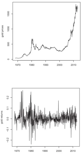
Figure I illustrates the evolution of the price of gold and gold returns over the sample period. The time-series plots demonstrate significant variations of the price of gold in the late 1970s and a clear bull market from 2002 - 2011. The strong fluctuations during the mid-seventies can be attributed to the the breakdown of Bretton Woods and the first major oil price shock.
*** Insert Figure I about here ***
10We have also considered the CBOE volatility index (VIX), however the corresponding time series starts
in 1986 and would therefore restrict our sample period. Thus, we make use of a GARCH(1,1) process of the returns of the MSCI world index as a proxy for the VIX, since the correlation between both series is fairly high.
Figure II presents the time-series of gold returns exceeding 5% and 10% thresholds for both negative and positive returns. The graphs demonstrate that volatility of gold returns clusters and that the volatility is relatively high around 1980 and 2010. The 10% graph provides particularly strong evi-dence for the clustering with almost no large absolute returns present in the 20-year period between 1985 and 2005.
*** Insert Figure II about here ***
The strong variation in gold returns and gold prices suggests that the factors influencing gold prices also vary over time.
4
Forecast Performance
The usefulness of gold price forecasts can be assessed based on different criteria: the simplest bench-mark includes a naive random walk forecast. Regardless of their simplicity, random walk forecasts have turned out to be a tough benchmark to beat when it comes to forecasting financial variables such as exchange rates (Meese and Rogoff, 1983) or stock prices where even sophisticated models and methods frequently fail to provide superior forecast.
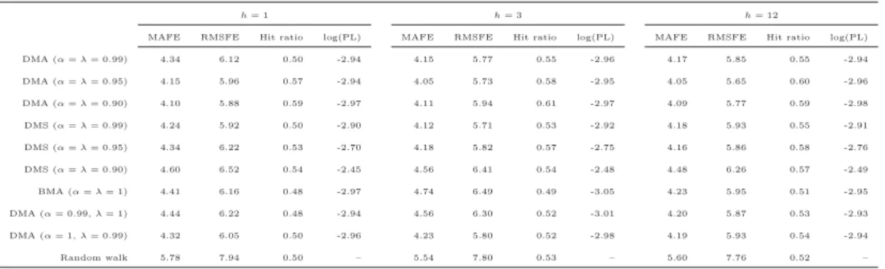
Table I reports some forecast error statistics at different forecast horizons (h= 1,3,12) for our DMA and DMS model in comparison to several alternatives including the simple random walk and other model averaging techniques, where either one or both forgetting factors are fixed. Another simple but useful benchmark is the “hit ratio” which corresponds to the percentage of correct direction forecasts. Such a measure is useful within portfolio decisions where the direction rather than the magnitude of the forecast matters. In addition, we do not only include classical forecast error criteria such as the mean absolute forecast error (MAFE) or the root mean squared forecast error (RMSFE), but we also consider a Bayesian criteria: the sum of the log predictive likelihood (log(PL)). This has the advantage that we do not only evaluate the point forecasts but also consider the entire predictive distributionf(yt|Yt−1).
*** Insert Table I about here ***
Overall, it becomes evident that a forecaster is better off using our flexible approach, which accounts for both model and parameter uncertainty. More precisely, Table I reveals that DMA or DMS with forgetting factors of at least 0.95 provides more accurate forecasts compared to less flexible alternatives such as BMA or DMA with a forgetting factor fixed to unity, i.e. no forgetting. In addition, for a forecast horizon of one month the sign of the gold return is predicted correctly in at least 50% of the cases while less flexible alternatives perform slightly worse. In addition, DMS seems to be superior compared to DMA for a slower forgetting of the past (e.g. forgetting factor of 0.99) while DMA appears to be better for a faster rate of forgetting (e.g. values of 0.95 or 0.90). Our overall evidence, that our approach is (1) clearly superior to a simple random walk and (2) flexible enough to outperform model averaging techniques that do not imply any forgetting (BMA) or do not allow for model and parameter uncertainty at the same time, also holds for higher forecast horizons. This is supported by both classical and Bayesian criteria. In the following section we discuss the posterior inclusion probabilities achieved by our approach with a relatively slow rate of forgetting (α= λ= 0.99) in order to show that the importance of several gold price determinants has changed over time.
5
Time-Varying Importance of Gold Price Determinants
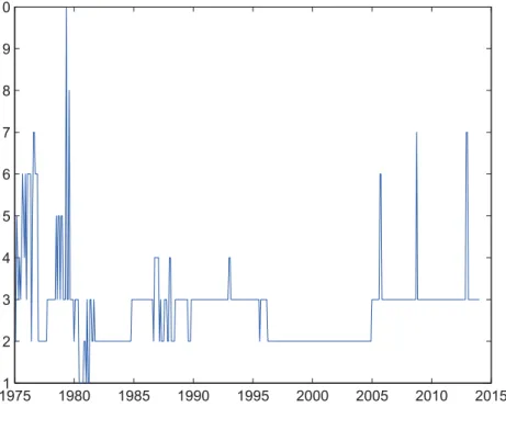
Figure III shows the time-varying number of predictors (including the constant) included in the model attached to the highest inclusion probability. The graph provides clear evidence that shrinkage is needed to provide accurate gold forecasts. In most cases, two or three regressors turn out to be the optimal choice. Once again, the high-volatility periods at the beginning and the end of the sample turn out to be exceptions. While frequent switches are observed at the beginning of the sample until the start of the eighties, the model also briefly includes six or seven regressors three times after 2005. It is quite remarkable that the algorithm drops down to three regressors almost immediately at each point in time. This demonstrates the flexibility and the learning of the DMA approach: More regressors are included to account for unexpected changes but a more parsimonious model is selected quickly afterwards.
*** Insert Figure III about here ***
Figures IV-VI provide the probability that a predictor is useful for forecasting at timetbased on the weight attached by DMA to models which include the corresponding regressor. An inspection of the different graphs suggests that the inclusion probability always exceeds 0.5 during at least one point in time, suggesting that each variable is important at some stage over the sample period. Interestingly, the importance of some variables such as the US consumer price index significantly decreases after the first years while other variables such as silver prices become increasingly important as time evolves. The overall high volatility of the probabilities during the beginning of the sample can be traced back to the economic turbulence after the first oil price shock.11
Many probabilities also show significant changes around the Millennium. Taking Figure II into ac-count, it becomes evident that periods of large absolute gold returns coincide with those changes in the inclusion probabilities. This demonstrates the flexibility of our forecasting approach since changing patterns of the gold price are reflected in changes of the weights attached to the different regressors. Furthermore, some regressors are favored once volatility of the gold price increases but the probabilities decrease again shortly afterwards, illustrating the feature of fast changing weights. We have already shown in the previous section that this flexibility pays off in terms of forecast accuracy compared to other averaging techniques.
Figure IV presents the posterior inclusion probabilities for the MSCI world stock market index, the S&P500 composite stock market index, the GARCH(1,1) of the MSCI stock returns, the S&P GSCI commodity price index, and silver prices. The stock market indices both exhibit inclusion probabilities clearly below 0.5 on average with the S&P500 index displaying larger but more volatile inclusion probabilities than the MSCI world index after 1995. The inclusion probabilities provide weak evidence for the importance of stock markets to forecast gold prices in general. There is also no significant evidence for an increased inclusion probability during financial crisis or turmoil consistent with gold’s safe haven status. More specifically, positive changes of the inclusion probabilities around the Asian financial crisis and the Russian crisis in 1997 and 1998 and the turmoil following the Lehman
11However, it is worth noting that the probabilities at the very beginning of the sample period should be
interpreted with caution, since these could depend on the choice of the initial conditions, i.e. noninformative prior on the model probabilities.
Brothers bankruptcy in 2008 are small and insignificant. The picture is different for the estimated GARCH volatility of the MSCI stock index returns. The inclusion probability is significantly higher compared to the return series and increases rapidly between 2000 and 2008. The GSCI commodity price index exhibits inclusion probabilities close to one around 2006 but stay below 0.5 for most parts of the sample. The results for the CRB display the same pattern but are more volatile at the beginning of the sample and are close to zero after. The inclusion probabilities for silver prices are mostly higher and more volatile with relatively high values between 1995 and 2005 but values below 0.5 at the end of the sample period.
The results for stock and commodity prices confirm that “systematic” factors are only partly im-portant to forecast gold prices. The overall pattern for stock prices suggests that in-sample (non-predictive) safe haven or hedge functions of gold against stocks which have been frequently established over the period under investigation are not necessarily related to out-of-sample predictive power. In addition, the safe haven effect is often more pronounced on a short-term basis and not significant for monthly data. These periods may thus be too short to gain weight in the inclusion probabilities of our monthly dataset.
*** Insert Figure IV about here ***
*** Insert Figure V about here ***
Figure V presents the posterior inclusion probabilities for the US consumer price index (CPI), a global (world) consumer price index as well as US long-term and short-term interest rates. The inclusion probabilities of the US CPI indicate that consumer prices have played a big role during the high inflation regimes in the 1970s and an insignificant role during the “great moderation” period between 1980 and mid-2000, in which inflation rates have been relatively low. The inclusion probabilities have increased from values of zero in 2000 to values close to 0.4 in 2013. This increase lends weight to the view that quantitative easing after the financial crisis in 2008 implies higher inflation expectations. In contrast, the global price index exhibits relatively large inclusion probabilities in the 1980s and
reduced and more volatile probabilities in the 1990s consistent with the lower inflation rates and expectations during the “great moderation”. Remarkably, the inclusion probabilities increase around 2005 and are slightly above 0.5 for the post-2008 crisis period. These findings support the inflation hedge property of gold at a global level and demonstrate that gold is rather influenced by world price levels than by US price levels.12
We analyze price levels and interest rates in one graph as these series generally co-move as predicted by the Fisher effect. We focus on US interest rates as a global benchmark. The inclusion probabilities for 10-year US government bond yields display an inclusion probability above 0.5 in the 1970s and increases after 1985 and 2000. The shorter maturity 3-month T-bill provides weaker evidence, i.e. lower and more volatile inclusion probabilities which decrease until 2000 but increase significantly afterwards and surpass the 10-year bonds at the end of the sample. A possible explanation for this pattern is that monetary policy currently faces a zero lower bound environment. The traditional role of long-term government bonds for anchoring inflation is less important since market participants pay more attention to short-run changes and announcements made by monetary authorities.
*** Insert Figure VI about here ***
Figure VI contains plots for the US dollar trade-weighted index, the euro trade-weighted index, the world FX reserves of central banks, and the Barclays capital aggregate bond index. All series yield relatively low inclusion probabilities for most of the sample period between 1980 and until 1995. The low inclusion probabilities between 1985 and 2000 might be surprising at first but less so if the high volatility of the US dollar relative to the gold price over this period is taken into account. Of all indices, world FX reserves display the highest probability at the end of the sample. This probably mirrors the fact that central banks, most notably, China and India, have only recently started to diversify their FX reserves and purchased gold. This might have resulted in expectations of ongoing gold purchases by central banks and is reflected in the low inclusion probabilities on average and the
12The causality pattern between gold returns and inflation is ambiguous. Considering that gold prices
incorporate inflation expectations, one might rather expect that gold forecasts inflation but not that inflation forecasts gold. However, a possible explanation for our findings is that changes in current inflation also introduce changes into expected inflation. An increase in expected inflation might then generate additional demand for gold as market participants use gold to hedge against higher inflation.
increase of the inclusion probabilities to values above 0.5 in the late 2000s.
Our results provide strong support for the time-variation of factors which drive the gold price. The most obvious pattern is that most regressors display inclusion probabilities close to zero between 1985 and 2000 when gold returns were low and the price of gold relatively constant. On the other hand, most inclusion probabilities increase significantly after 1995 when the gold price becomes more volatile. The large variation in the probabilities suggests that simple averaging over all models is an inadequate strategy since this would result in equal and constant weights for all models (as mirrored by the prior) over the full sample period. The results also emphasize that a model that focuses on gold price forecasts provides different results compared to models that focus on the factors that influence the price of gold contemporaneously and thus in-sample. For example, exchange rates exhibit a strong contemporaneous, in-sample effect but essentially no predictive, out-of-sample effect.
6
Summary and Concluding Remarks
This paper proposes Dynamic Model Averaging to forecast the price of gold and contributes to the gold economics literature with a novel econometric methodology to forecast gold prices. The paper stresses that accounting for both model and parameter uncertainty is particularly important for an asset for which no pricing model exists and that is influenced by a variety of local and global factors that potentially change over time.
The estimation results show that parsimonious forecasting models with only three variables clearly dominate richer models with up to fourteen variables. However, it becomes also clear that the inclusion of more predictors is beneficial due to the fact that our averaging approach is more flexible to capture abrupt changes. In addition, the factors that influence future gold prices vary significantly through time and can be clearly distinguished from results that focus on the in-sample and non-predictive relationships within a classical regression model. More precisely, we find that in-sample functions of gold such as the safe haven property, the currency hedge property or portfolio diversifier property do not automatically translate into out-of-sample predictability. The results also show that the Dynamic Model Averaging approach outperforms alternatives such as the random walk and Bayesian Model Averaging. An appealing feature of DMA is its ability to learn and its flexibility in terms of the
weights attached to regressors: as an example, periods of large gold returns coincide with rapid changes of the inclusion probabilities.
An interesting avenue for future research could be an analysis of the usefulness of gold prices for fore-casting stocks, bonds, exchange rates or inflation rates within a Dynamic Model Averaging framework.
References
Baker, S.A. and R.C. Van Tassel (1985), Forecasting the Price of Gold: A Fundamentalist Approach, Atlantic Economic Journal, 13(4), 43-52.
Batten, J.A., C. Ciner, and B.M. Lucey (2014), On the Economic Determinants of the Gold-Inflation Relation, Resources Policy, 41, 101-108.
Baur, D.G. and B.M. Lucey (2010), Is Gold a Hedge or a Safe Haven? An Analysis of Stocks, Bonds and Gold, The Financial Review, 45, 217-229.
Beckmann, J. and R. Czudaj (2013), Gold as an Inflation Hedge in a Time-Varying Coefficient Framework, The North American Journal of Economics and Finance, 24, 208-222.
Blose, L.E. (2010), Gold Prices, Cost of Carry, and Expected Inflation, Journal of Economics and Business, 62(1), 35-47.
Capie, F., T.C. Mills, and G. Wood (2005), Gold as a Hedge against the Dollar, Journal of Interna-tional Financial Markets, Institutions and Money 15(4), 343-352.
Deckers, T. and C. Hanck (2014), Variable Selection in Cross-Section Regressions: Comparisons and Extensions, Oxford Bulletin of Economics and Statistics, forthcoming.
Escribano, A. and C. Granger (1998), Investigating the Relationship between Gold and Silver Prices, Journal of Forecasting, 17, 81-107.
Jastram, R.W. (2009), The Golden Constant: The English and American Experience 1560-2007, (with updated material by Jill Leyland), Edward Elgar.
Koop, G. and D. Korobilis (2012), Forecasting Inflation using Dynamic Model Averaging, Interna-tional Economic Review, 53, 867-886.
Meese, R.A. and K. Rogoff (1983), Empirical Exchange Rate Models of the Seventies: Do they fit out of Sample?, Journal of International Economics, 14(1-2), 3-24.
Pierdzioch, C., M. Risse, and S. Rohloff (2014), On the Efficiency of the Gold Market: Results of a Real-Time Forecasting Approach, International Review of Financial Analysis, 32, 95-108. Raftery, A.E. (1995), Bayesian Model Selection in Social Research, Sociological Methodology, 25,
111-163.
Raftery, A.E., Karny, M. and P. Ettler (2010), Online Prediction under Model Uncertainty via Dynamic Model Averaging: Application to a Cold Rolling Mill, Technometrics, 52(1), 52-66. Rossi, B. (2005), Testing Long-Horizon Predictive Ability with High Persistence, and the
Meese-Rogoff Puzzle, International Economic Review, 46(1), 61-92.
Sherman, E. (1982). Gold: A Conservative, Prudent Diversifier, Journal of Portfolio Management, 8(3), 21-27.
Sjaastad, L. A. and F. Scacciavillani (1996). The Price of Gold and the Exchange Rates, Journal of International Money and Finance 15, 879-897.
Figure I Gold prices and gold returns
This Figure presents the evolution of monthly gold prices (top panel) and monthly gold
returns (bottom panel). The plots illustrate significant variation of the gold price through
time.
1970 1980 1990 2000 2010 0 500 1000 1500 gold pr ices 1970 1980 1990 2000 2010 − 0.2 − 0.1 0.0 0.1 0.2 gold retur nsFigure IILarge absolute gold returns
The plots show the largest positive and negative gold returns if absolute returns exceed 5%
(top plot) and 10% thresholds (bottom plot). The graphs clearly indicate volatility clustering
in particular in the 1970s and in the post-2008 period.
1970 1980 1990 2000 2010 − 0.2 − 0.1 0.0 0.1 0.2 gold retur ns > 5% 1970 1980 1990 2000 2010 − 0.2 − 0.1 0.0 0.1 0.2 gold retur ns > 10%
Figure IIIOptimal model size
The graph shows the time-varying number of predictors (including the constant) included in
the model attached to the highest inclusion probability.
19751 1980 1985 1990 1995 2000 2005 2010 2015 2 3 4 5 6 7 8 9 10
Figure IVDMA posterior inclusion probabilities for stock prices and commodity prices
The plots show the posterior inclusion probabilities for the MSCI world stock market index,
the S&P500 composite stock market index, the GARCH(1,1) process of the returns of the
MSCI world index (proxy for the VIX), the S&P GSCI commodity price index, the CRB
commodity price index, and silver prices. The graphs provide the probability that a predictor
is useful for forecasting at time
t
based on the weight attached by DMA to models which
include the corresponding regressor.
MSCI
S&P
19750 1980 1985 1990 1995 2000 2005 2010 2015 0.1 0.2 0.3 0.4 0.5 0.6 0.7 πt 19750 1980 1985 1990 1995 2000 2005 2010 2015 0.1 0.2 0.3 0.4 0.5 0.6 0.7 πtGARCH(1,1)
S&P GSCI
19750 1980 1985 1990 1995 2000 2005 2010 2015 0.1 0.2 0.3 0.4 0.5 0.6 0.7 0.8 πt 19750 1980 1985 1990 1995 2000 2005 2010 2015 0.1 0.2 0.3 0.4 0.5 0.6 0.7 0.8 πt
CRB
Silver
19750 1980 1985 1990 1995 2000 2005 2010 2015 0.1 0.2 0.3 0.4 0.5 0.6 0.7 πt 19750 1980 1985 1990 1995 2000 2005 2010 2015 0.1 0.2 0.3 0.4 0.5 0.6 0.7 0.8 0.9 1 πtFigure VDMA posterior inclusion probabilities for consumer prices and interest rates
The plots show the posterior inclusion probabilities for the US consumer price index, a global
(World) consumer price index and US long-term and short-term interest rates.
US CPI
W CPI
19750 1980 1985 1990 1995 2000 2005 2010 2015 0.1 0.2 0.3 0.4 0.5 0.6 0.7 0.8 0.9 1 πt 19750 1980 1985 1990 1995 2000 2005 2010 2015 0.1 0.2 0.3 0.4 0.5 0.6 0.7 0.8 0.9 1 πtlong-term
short-term
1975 1980 1985 1990 1995 2000 2005 2010 2015 0.2 0.25 0.3 0.35 0.4 0.45 0.5 0.55 0.6 0.65 πt 19750 1980 1985 1990 1995 2000 2005 2010 2015 0.1 0.2 0.3 0.4 0.5 0.6 0.7 0.8 πtFigure VIDMA posterior inclusion probabilities for effective dollar FX rate and world FX reserves
The plots show the posterior inclusion probabilities for the US dollar trade-weighted index,
the world FX reserves of central banks, the euro trade-weighted index, and the Barclays
Capital US aggregate bond index.
US dollar
FX reserves
19750 1980 1985 1990 1995 2000 2005 2010 2015 0.1 0.2 0.3 0.4 0.5 0.6 0.7 πt 19750 1980 1985 1990 1995 2000 2005 2010 2015 0.1 0.2 0.3 0.4 0.5 0.6 0.7 0.8 0.9 1 πtEuro
US Bonds
19750 1980 1985 1990 1995 2000 2005 2010 2015 0.1 0.2 0.3 0.4 0.5 0.6 0.7 πt 19750 1980 1985 1990 1995 2000 2005 2010 2015 0.05 0.1 0.15 0.2 0.25 0.3 0.35 0.4 0.45 0.5 πtTable IComparison of forecast models
h= 1 h= 3 h= 12
MAFE RMSFE Hit ratio log(PL) MAFE RMSFE Hit ratio log(PL) MAFE RMSFE Hit ratio log(PL) DMA (α=λ= 0.99) 4.34 6.12 0.50 -2.94 4.15 5.77 0.55 -2.96 4.17 5.85 0.55 -2.94 DMA (α=λ= 0.95) 4.15 5.96 0.57 -2.94 4.05 5.73 0.58 -2.95 4.05 5.65 0.60 -2.96 DMA (α=λ= 0.90) 4.10 5.88 0.59 -2.97 4.11 5.94 0.61 -2.97 4.09 5.77 0.59 -2.98 DMS (α=λ= 0.99) 4.24 5.92 0.50 -2.90 4.12 5.71 0.53 -2.92 4.18 5.93 0.55 -2.91 DMS (α=λ= 0.95) 4.34 6.22 0.53 -2.70 4.18 5.82 0.57 -2.75 4.16 5.86 0.58 -2.76 DMS (α=λ= 0.90) 4.60 6.52 0.54 -2.45 4.56 6.41 0.54 -2.48 4.48 6.26 0.57 -2.49 BMA (α=λ= 1) 4.41 6.16 0.48 -2.97 4.74 6.49 0.49 -3.05 4.23 5.95 0.51 -2.95 DMA (α= 0.99,λ= 1) 4.44 6.22 0.48 -2.94 4.56 6.30 0.52 -3.01 4.20 5.87 0.53 -2.93 DMA (α= 1,λ= 0.99) 4.32 6.05 0.50 -2.96 4.23 5.80 0.52 -2.98 4.19 5.93 0.54 -2.94 Random walk 5.78 7.94 0.50 – 5.54 7.80 0.53 – 5.60 7.76 0.52 –
Note:The table reports the mean absolute forecast error (MAFE), the root mean squared forecast error (RMSFE), the hit ratio, and the sum of the log predictive likelihood (log(PL)) for each model alternative.