Advances in Measurement Error Modeling

Southern Methodist University

SMU Scholar

Statistical Science Theses and Dissertations Statistical Science

Spring 5-19-2019

Advances in Measurement Error Modeling

Linh Nghiem

[email protected]

Follow this and additional works at:https://scholar.smu.edu/hum_sci_statisticalscience_etds Part of theStatistical Methodology Commons, and theStatistical Models Commons

This Dissertation is brought to you for free and open access by the Statistical Science at SMU Scholar. It has been accepted for inclusion in Statistical Science Theses and Dissertations by an authorized administrator of SMU Scholar. For more information, please visithttp://digitalrepository.smu.edu. Recommended Citation

Nghiem, Linh, "Advances in Measurement Error Modeling" (2019).Statistical Science Theses and Dissertations. 6.

Advances in Measurement Error Modeling

Approved by:

Cornelis Potgieter

Assistant Professor of Statistical Science

Lynne Stokes

Professor of Statistical Science

Daniel Heitjan

Professor of Statistical Science

Jing Cao

Associate Professor of Statistical Science

Pankaj Choudmary

Advances in Measurement Error Modeling

A Dissertation Presented to the Graduate Faculty of Dedman College

Southern Methodist University in

Partial Fulfillment of the Requirements of the degree of

Doctor of Philosophy with a

Major in Statistical Science by

Linh Nghiem

B.S.B.A., Finance and Mathematics, University of Miami

Copyright (2019) Linh Nghiem All Rights Reserved

Nghiem, Linh B.S in Business Administration, University of Miami

Advances in Measurement Error Modeling Advisor: Dr. Cornelis Potgieter

Doctor of Philosophy conferred May 18, 2019 Dissertation completed April 30, 2019

Measurement error in observations is widely known to cause bias and a loss of power when fitting statistical models, particularly when studying distribution shape or the rela-tionship between an outcome and a variable of interest. Most existing correction methods in the literature require strong assumptions about the distribution of the measurement error, or rely on ancillary data which is not always available. This limits the applicability of these methods in many situations. Furthermore, new correction approaches are also needed for high-dimensional settings, where the presence of measurement error in the covariates adds another level of complexity to the desirable structure of the models, such as sparsity. This dissertation presents new correction methods for measurement error in two important statistical problems: density deconvolution and errors-in-variables models. For both density deconvolution and linear errors-in-variables regression, new estimators based on the empirical phase function are proposed. Compared to the existing methods, phase function-based estimators require only mild assumptions about the measurement error distribution. For high-dimensional errors-in-variables models, a new estimator that extends the flexible Simulation-Extrapolation (SIMEX) correction procedure is proposed in order to achieve sparsity of the solution. All the new estimators have been shown to have strong theoretical support and good finite sample performance. Data examples are provided to illustrate the practical use of each estimator in reality.

Contents

List of Figures vii

List of Tables ix

Acknowledgements xiii

1 Introduction 1

2 Density Deconvolution with Unknown Heteroscedastic Measurement Error 6

2.1 Overview . . . 6

2.2 Introduction . . . 7

2.3 Phase Function Estimation . . . 9

2.4 Density Estimation . . . 18

2.5 Analysis of Framingham Data . . . 29

2.6 Conclusions . . . 30

2.7 Appendix . . . 31

3 Linear Errors-in-Variables Estimation with Unknown Error Distribution 46 3.1 Overview . . . 46

3.2 Introduction . . . 46

3.3 Phase Function Minimum Distance Estimation . . . 48

3.4 Computational Considerations . . . 54

3.5 Simulation Study . . . 58

3.6 Air Quality Data Examples . . . 65

3.7 Conclusion . . . 68

3.8 Appendix . . . 69

4 SIMSELEX: Estimation in High-Dimensional Errors-in-Variables Model 86 4.1 Overview . . . 86

4.2 Introduction . . . 86

4.3 The SIMSELEX Estimator . . . 90

4.4 Model Illustration and Simulation Results . . . 95

4.5 SIMSELEX for Spline-Based Regression . . . 107

4.7 Conclusion . . . 118 4.8 Appendix . . . 119

5 Summary and Future Directions 132

5.1 Summary . . . 132 5.2 Future Directions . . . 132

List of Figures

Figure 2.1 Curves Q1 ( ), Q2 ( ), Q3 ( ), and true curve ( ) for X ∼ Scaled-χ2

3, n = 500, J = 2 replicates per observation when the errors are Normal (a)-(c), and Laplace (d)-(f), with case 1 of measurement error variances. For (a),(d): EPF estimator; (b),(e): WEPFopt estima-tor; (c),(f): D&M estimator with estimated variances. All estimators are computed using plug-in bandwidth discussed in Section 2.4.2 . . . 27 Figure 2.2 Curves Q1 ( ), Q2 ( ), Q3 ( ), and true curve ( )

for X ∼ Mixture 1, n = 500, J = 2 replicates per observation, when the errors are Normal (a)-(c), and Laplace (d)-(f), with case 1 of measurement error variances. For (a),(d): EPF estimator; (b),(e): WEPFopt estima-tor; (c),(f): D&M estimator with estimated variances. All estimators are computed using plug-in bandwidth discussed in Section 2.4.2. . . 28 Figure 2.3 Estimation of the density fX in the Framingham data. Four

den-sity estimates are shown: a naive kernel estimator (measurement error is ignored), the EPF estimator, the WEPFopt estimator, and the Delaigle &

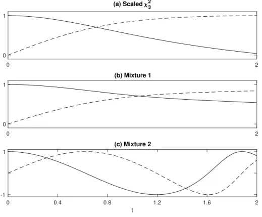
Meister estimator assuming Laplace measurement error. . . 30 Figure 2.4 Phase functions of the three distributions considered in the

simu-lation studies in Sections 2 and 3, real component ( ) and imaginary component ( ). . . 37 Figure 2.5 Curves Q1 ( ), Q2 ( ), Q3 ( ), and true curve ( )

for X ∼ Mixture 2, n = 500, with J = 2 replicates per observation, when the errors are Normal (a)-(c), and Laplace (d)-(f), with case 1 of mea-surement error variances. For (a),(d): EPF estimator; (b),(e): WEPFopt estimator; (c),(f): D&M estimator with estimated variances. All estima-tors are computed using plug-in bandwidth. . . 41 Figure 3.1 Time series plots for carbon monoxide Yt (top) and the average

sensor outputWt (bottom). . . 67

Figure 3.2 Kernel Density Estimators for W (new method) and Y (YGP method) data . . . 82 Figure 4.1 SIMSELEX illustration using microarray data (Section 5). Left

fig-ure: solid and dashed lines represent the norms||Γj||2 of, respectively, the selected and (some) unselected genes; the vertical dash-dot line is the one-se cross-validation tuning parameter. Right figure: coefficients of one-selected genes are modeled quadratically inλ and then extrapolated to λ=−1. . 95

Figure 4.2 Curves Q1 ( ), Q2 ( ), Q3 ( ), and true function ( ) for the esimated functions from the naive estimators (top) and the SIMSELEX estimators (bottom) corresponding top= 600 andσ_u2 = 0.15. For (a),(e): f1(x) = 3 sin(2x)+sin(x); for (b),(f): f2(x) = 3 cos(2πx/3)+x; for (c), (g): f3(x) = (1−x)2−4; for (d), (h): f4(x) = 3x. . . 114 Figure 4.3 Curves Q1 ( ), Q2 ( ), Q3 ( ), and true function

( ) for the esimated functions from the naive estimators (top) and the SIMSELEX estimators (bottom) corresponding top= 600 andσ2

u = 0.30.

For (a),(e): f1(x) = 3 sin(2x)+sin(x); for (b),(f): f2(x) = 3 cos(2πx/3)+x; for (c), (g): f3(x) = (1−x)2−4; for (d), (h): f4(x) = 3x. . . 115 Figure 4.4 Elbow plots choosing tuning parameters in implementation of

List of Tables

Table 2.1 The ratio MSEeq/MSEopt and the corresponding jackknife standard

error (in parentheses) when estimating the phase function ofXwith normal measurement error and variance structure given in Case 1 of Table 2.2, based onN = 1000 samples, when there are no replicate (assuming the true variances of measurement errors are known), 2 replicates, and 3 replicates per observation. . . 15 Table 2.2 Three measurement error variance structures used in simulations. . 16 Table 2.3 The effect of the error variance structure on the ratio MISEeq/MISEopt

and the corresponding jackknife standard error (in parentheses) based on 1000 samples of size n= 1000. . . 17 Table 2.4 Density estimation forn = 500 with no replicates and measurement

error variances are assumed to be known. The median, as well as first and third quartiles, [Q1, Q3], of 10 × ISE of density estimators under 500 simulations. . . 23 Table 2.5 Density estimation for n = 500 with J = 2 replicates for each

observation. The median, as well as first and third quartiles, [Q1, Q3], of 10× ISE of density estimators under 500 simulations. . . 24 Table 2.6 The median and [Q1, Q3] of 10×ISE of the density estimators with

optimal bandwidth based on 500 simulations. Each simulation has sample size n= 500 with no replicate (measurement error variances are known). 42 Table 2.7 The median and [Q1, Q3] of 10×ISE of the density estimators with

optimal bandwidth based on 500 simulations. Each simulation has sample size n= 500 and J = 2 replicates per observation. . . 43 Table 2.8 The median and [Q1, Q3] of 10×ISE of the density estimators with

plug-in bandwidth based on 500 simulations. Each simulation has sample size n= 500 and J = 3 replicates per observation. . . 44 Table 2.9 The median and [Q1, Q3] of 10×ISE of the density estimators with

optimal bandwidth based on 500 simulations. Each simulation has sample size n= 500 and J = 3 replicates per observation. . . 45 Table 3.1 Ratio of median square error of estimators relative to the

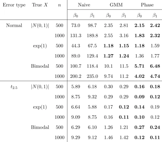
disattenu-ated regression estimators in the univariate model simulation with model errors being Normal andt2.5 distributions. Note GMM stands for general-ized method of moments. . . 61

Table 3.2 Median square error of the generalized method of moments estima-tors, denoted GMM in the table, and the phase function estimators when the model errors are Cauchy. . . 62 Table 3.3 Ratio of median square error of estimators relative to the

simulation-extrapolation regression estimators in the bivariate model simulation. . . 64 Table 3.4 True standard error (Monte Carlo) and median of estimated

stan-dard error, scaled by the square root of the sample size, using two different bootstrap approaches. . . 65 Table 3.5 n×median{SE} and the corresponding interquartile range for the

phase function estimators with weighting functionsK1(t), K2(t), and K3(t). 73 Table 3.6 Median square errors of estimators and the corresponding

interquar-tile range (in parentheses), scaled by the sample size, in the univariate regression simulation when the true distribution ofX is half-normal. . . . 75 Table 3.7 Median square errors of estimators and the corresponding

interquar-tile range (in parentheses), scaled by the sample size, in the univariate regression simulation when the true distribution ofX is exponential. . . . 76 Table 3.8 Median square errors of estimators and the corresponding

interquar-tile range (in parentheses), scaled by the sample size,in the univariate re-gression simulation when the true distribution ofX is a mixture of normal distributions. . . 77 Table 3.9 Median square error and interquartile range of the GMM and phase

function estimators in the univariate regression simulation when model errors are Cauchy . . . 78 Table 3.10 Median square error and interquartile range (in parentheses), scaled

by the sample size for the estimators in the multivariate regression sim-ulation when X and Z are half-normal and correlated with correlation

ρ=.5. . . 79 Table 3.11 Median square error and interquartile range (in parentheses), scaled

by the sample size, for the estimators in the multivariate regression simu-lation when X and Z are mixtures of normal distribution and correlated with correlation ρ=.5. . . 80 Table 3.12 Naive, GMM, and phase function-based estimators of the linear

errors-in-variables for the abrasiveness index data. . . 81 Table 3.13 Analysis of different measurements in the OPEN study . . . 84 Table 4.1 Comparison of estimators for linear regression with with the case

of θ1 based on `2 estimation error, average number of false positives (FP) and false negatives (FN). Standard errors in parentheses. . . 99

Table 4.2 Comparison of estimators for logistic regression with with the case of θ1 based on `2 estimation error, average number of false positives (FP) and false negatives (FN). Standard errors in parentheses. . . 102 Table 4.3 Comparison of estimators for Cox survival models for the case θ1

based on `2 estimation error, average number of false positives (FP) and false negatives (FN). Standard errors in parentheses. . . 105 Table 4.4 Comparison of SIMSELEX variable selection methods for spline

re-gression withp= 100. . . 112 Table 4.5 Comparison of estimators for high-dimensional spline regression model

based on estimation error (MISE), average number of false positives (FP) and false negatives (FN). Standard errors in parentheses. . . 113 Table 4.6 Gene symbols and estimated coefficients from the naive lasso, the

conditional scores lasso, and the SIMSELEX estimator applied to the Wilms tumors data. Genes selected by SIMSELEX are printed in bold. . 117 Table 4.7 Comparison of estimators for linear regression with with the case

of θ2 based on `2 estimation error, average number of false positive (FP), and average number of false negative (FN) across 500 simulations. . . 125 Table 4.8 Comparison of estimators for logistic regression with with the case

of θ2 based on `2 estimation error, average number of false positive (FP), and average number of false negative (FN) across 500 simulations. . . 126 Table 4.9 Comparison of estimators for Cox survival models for the case θ2

based on`2estimation error, average number of false positive (FP), average number of false negative (FN) across 500 simulations. . . 127 Table 4.10 Monte Carlo mean and median `2 error of SIMSELEX estimator

using nonlinear means (NL) and quadratic (Quad) extrapolation function for linear and logistic regression. . . 128 Table 4.11 Comparison of SIMSELEX and post-selection SIMEX estimators

using mean `2 error for linear and logistic model. Nonlinear (Nonlin) and quadratic (Quad) extrapolation were considered. . . 130 Table 4.12 Median computation time (in second) for different estimators. For

the conditional score lasso and GMUS it is the median time to generate a coefficient path with 25 values of the tuning parameter. . . 131

Acknowledgements

I would like to express my deepest gratitude to many people who have taught, helped, supported, and mentored me during my time at Southern Methodist University (SMU). My past four years at SMU was full of both joyful and challenging moments; together, they have made a long-lasting impact in my career and my life.

I am indebted to the generous support of my advisor, Cornelis Potgieter. Not only he mentored me tirelessly on how to do research and helped me considerably in my job application, but his great dedication to student is also an excellent example for me to follow in my career. In 2018, although having many life and career incidents, he did not let them prevent him from being positive and energetic in every conversation with me, other students and colleagues. Such an attitude deeply influenced me and will continue to shape me in the future. Thanks again, Nelis!

In my first year of the PhD program, my beloved mother passed away during an accident in a minor surgery. I couldnt overcome this tremendous loss without the support of the faculty and my classmates; they were always with me when I needed help, both academically and emotionally. Even after many months later, they still asked about how my family was doing and shared my sorrows on the first Christmas after my mothers death. These supports meant a lot to me and motivated me not to give up at that difficult time.

During the PhD program, I also had the pleasure of collaborating with many other Statistics faculty and classmates on the projects that may or may not be directly related to the thesis. Particularly, I am thankful to collaborating and writing papers with Michael Byrd in three research projects. Our tons of ad-hoc discussions in the office and through the Google Hangout clarified many issues and helped us learn from each other very well. Furthermore, I am very grateful to the experience of working in diverse roles that the

department offered me. In addition to doing research on statistical methodology, I had opportunities to work as a statistical consultant, a teaching assistant, and a tutor working with student on one-to-one basis. These experience improved my statistical communica-tion to a wide range of audiences and opened up many interdisciplinary collaboracommunica-tions that bring statistics into real lives.

During my stay at SMU and Dallas, I made some great friends and my life would not have been the same without them. I would like to thank Michael Byrd, Thomas Crutcher and Emily Boak for our meals at a ton of places in Dallas, especially when you let me go to Asian places most of the time. Thank you Chinh Nguyen, Duyen Le, Duc Truong, Kathy Le, Thao Nguyen, Ngoan Tran, Luan Vu, Tu-Anh Tran, Ly Nguyen, Hiep Tran, Duc Vu, Minh Nguyen, for delicious Vietnamese food and countless parties. Thank you many Vietnamese friends around the US who hosted and traveled with me around the United States. Any many others who have interacted and supported me in this wonderful adventure.

Finally, I would like to thank my parents and my family for their endless and uncon-ditional love and support. When my mother was alive, she strongly supported me to pursue the PhD and an academic career. Although my career journey is still far ahead with many uncertainties, I hope at this point she is smiling proudly from the heaven.

Chapter 1 Introduction

Statistics is the science of collecting, visualizing, and analyzing data. However, data are obtained from measurement processes that are subject to errors. The sources of measurement error can range from the lack of accuracy in the instruments used to measure variables to the inadequacy of short-term measurements for long-term variables. As a result, it is common that the obtained data are not samples of the variables of interests, but consist of contaminated versions of these variables. Broadly speaking, measurement error modeling refers to statistical models that correct for measurement errors in such scenarios.

Measurement errors are well-known to have a substantial impact on statistical models. Particularly, the impacts are most serious when trying to understand the effect of the variable of interest on a specific measured outcome, or when trying to understand the shape of the population distribution of the variable of interest. In general, measurement errors cause bias and loss of power in statistical models. For example, consider the simple linear regression model, Y =β0 +β1X+ε, and the data consists of pairs (Yi, Wi) with

Wi = Xi +Ui, i = 1, . . . , n, with Ui being the measurement error for observation i. If

measurement error is ignored, regression ofY onW results in an inconsistent estimator of both the intercept β0 and the slopeβ1, see Carroll et al. (2006). Therefore, measurement error should be accounted for to understand the true relationship between Y and X.

The above example represents a typical errors-in-variables (EIV) models. In such models, the general interest is to model an outcome of interest Y as a function of

p1−dimensional error-prone covariates X and p2-dimensional error-free covariates Z. The function is usually involved some some parameters Θ. However, the observed sample consists of measurements (W1,Z1, Y1), . . . ,(Wn,Zn, Yn), withWi =Xi+Ui,i= 1, . . . , n

where the measurement errors vector Ui are assumed to have mean zero and covariance

matrix Σu. The parameter Θ can be finite dimensional, such as in the case of linear and

generalized linear models, Cox survival models, or infinite dimensional, such as in the case of nonparametric regression models.

Most popular correction methods for measurement errors in EIV models require strong distributional assumptions or potentially unavailable auxiliary data for model estimation. Specifically, it is generally assumed that the covariance matrix Σu is known. In the simple

linear regression case (p1 = 1 and p2 = 0), a consistent and unbiased estimator of the slopeβ1 is obtained as ˆβ1 = ˆβ1WσX2/(σX2 +σU2), where ˆβ1W is the estimated slope obtained by regressingY onW. Calculation of this estimator requires that the variance of measure-ment errorσ2

U be known or estimable. In the multiple predictor setting, there is generally

no closed-form solution for the corrected estimator. Instead, simulation-extrapolation (SIMEX), first proposed by Stefanski and Cook (1995) and K¨uchenhoff et al. (2006), is frequently used. The SIMEX procedure evaluates the effects of measurement error on the estimator by increasing the level of measurement error through a simulation step, and then extrapolating to the setting of no measurement error. SIMEX also requires that Σu be known or estimable. Another approach to correcting for measurement error

is regression calibration, see Carroll and Stefanski (1990). Here, a regression of X onW

is used to estimate X, say ˆX, and then the linear model parameters are estimated by regressing Y on ˆX. The regression of X on W is assumed to be available through an either validation data or an instrumental variable T.

When the distributions of X and U are fully specified, likelihood methods can also be used to estimate parameters, see Schafer and Purdy (1996) and Higdon and Schafer (2001). Implementation of these likelihood methods generally requires the use of numeri-cal methods such as Gaussian quadrature or Monte Carlo integration. The EM algorithm of Dempster et al. (1977) can also be used. An approach that does not require the distri-bution ofX to be known is the conditional score method of Stefanski and Carroll (1987). However, this method does require that both parametric models for Y|X and W|X be specified.

For the linear EIV models where Y = Xβ +ε, W = X +U, another approach to estimating coefficientsβ is based on the method of moments, dating back to the work of Reiersøl (1941), who estimated the slope of the simple EIV model through third-order moments. Gillard (2014) considered slope estimators based on third and fourth moments, and finds these to have large variances. More recently, methods based on the matching of higher-order moments (or variants such as cumulants) have been explored with renewed interest. Erickson and Whited (2002) expressed high-order residual moments as nonlin-ear functions of both coefficients and nuisance parameters, while Erickson et al. (2014) expressed the third and fourth residual cumulants as a linear function of the coefficients. The latter also established that the two methods were asymptotically equivalent. The method of moments approach is nonparametric, in that it does not require parametric distributions to be specified for any of the components. However, an implementation based on the first M sample moments generally requires 2M finite population moments. In high dimensional setting, the presence of measurement error introduces an added layer of complexity and can have severe consequences on the lasso estimator: the num-ber of non-zero estimates can be inflated, sometimes dramatically, and as such the true sparsity pattern of the model is not recovered, see Rosenbaum et al. (2010). Several methods have been proposed that correct for measurement error in high-dimensional set-ting. Rosenbaum et al. (2010) proposed a matrix uncertainty selector (MU) for additive measurement error in the linear model. Rosenbaum et al. (2013) proposed an improved version of the MU selector, and Belloni et al. (2017) proved its near-optimal minimax properties and developed a conic programming estimator that can achieve the minimax bound. The conic estimators require selection of three tuning parameters, a difficult task in practice. Another approach for handling measurement error is to modify the loss and conditional score functions used with the lasso, see Sørensen et al. (2015) and Datta et al. (2017). Additionally, Sørensen et al. (2018) developed the generalized matrix un-certainty selector (GMUS) for the errors-in-variables generalized linear models. Both the conditional score approach and GMUS require the subjective choice of tuning parameters. The second problem where it is important to correct for measurement errors is in

density estimation. This problem is often referred to asdensity deconvolution. When the noise-to-signal ratio is large, implementing a correction becomes crucial as the density of the observed data can deviate substantially from the true density of interest. Let fX(x)

denote the density function of a random variable X, and assume that it is of interest to estimatefX(x) whenXis not directly observable. Specifically, we are only able to observe

contaminated versions of X, say W = X+U, where U represents measurement error. Thus, we are interested in estimating the density function of X based on an observed sample W1, W2, ..., Wn with Wi = Xi +Ui, i = 1, . . . , n. Here, the Xi are an iid sample

from a distribution with density fX, with Ui representing the measurement error of the

ith _{observation. The U}

i are assumed both mutually independent and independent of the

Xi.

The nonparametric density deconvolution problem when first considered assumed that the distribution of the measurement error was fully known, see Carroll and Hall (1988) and Stefanski and Carroll (1990). The development that followed in the literature mostly considered the case of known measurement error, and generally treated the measurement error as homoscedastic, including Fan (1991a), Fan (1991b), Fan and Truong (1993), Hall and Qiu (2005), Lee et al. (2010). The case of heteroscedastic measurement error was considered by Fan (1992) and Delaigle and Meister (2008). The problem of the measure-ment error having an unknown distribution was considered by Diggle and Hall (1993) and Neumann and H¨ossjer (1997) who assumed that samples of error data are available, and by Delaigle et al. (2008) who used replicate data to estimate the entire character-istic function of the measurement error. McIntyre and Stefanski (2011) considered the heteroscedastic case with replicate observations. Their work assumed the measurement errors all follow a normal distribution with unknown variances only. The phase function deconvolution approach developed by Delaigle and Hall (2016) is groundbreaking in that they estimate the density functionfX with both the measurement error distribution and

variance unknown, and without the need for replicate data. Their method is based on minimal assumptions: The measurement error terms Ui are only assumed to be

function. However, Delaigle and Hall (2016) only considered the case where the Ui are

homoscedastic, while heteroscedastic data is a reality often encountered in practice. In fact, the variance of measurement error often increases with the true underlying value, see Guo and Little (2011).

This thesis proposes new estimators based on the empirical phase functions and a new estimation procedure for errors-in-variables models in high dimensional settings. Specifically, in chapter 2, we develop a new density deconvolution estimator when the measurement errors are heteroscedastic of unknown type. In chapter 3, we apply the phase function method to linear errors-in-variables (EIV) models. In chapter 4, we propose a new estimation procedure that augments the traditional SIMEX for EIV models in high dimensional settings. Chapter 5 concludes the thesis with a brief summary and future direction.

Chapter 2

Density Deconvolution with Heteroscedastic Measurement Error of Unknown Type

2.1. Overview

This chapter considers the problem of density estimation when the measurement er-ror is present. The density estimators that adjust for measurement erer-ror are broadly referred to as density deconvolution estimators. While most methods in the literature assume the distribution of the measurement error to be fully known, a recently proposed method based on the empirical phase function (EPF) can deal with the situation when the measurement error distribution is unknown. The EPF density estimator has only been considered in the context of additive and homoscedastic measurement error; how-ever, the measurement error of many biomedical variables is heteroscedastic in nature. In this chapter, we developed a phase function approach for density deconvolution when the measurement error has unknown distribution and is heteroscedastic. A weighted em-pirical phase function (WEPF) is proposed where the weights are used to adjust for het-eroscedasticity of measurement error. The asymptotic properties of the WEPF estimator are evaluated. Simulation results show that the weighting can result in large decreases in mean integrated squared error (MISE) when estimating the phase function. The estima-tion of the weights from replicate observaestima-tions is also discussed. Finally, the construcestima-tion of a deconvolution density estimator using the WEPF is compared to an existing de-convolution estimator that adjusts for heteroscedasticity, but assumes the measurement error distribution to be fully known. The WEPF estimator proves to be competitive, especially when considering that it relies on minimal assumption of the distribution of measurement error.

2.2. Introduction

Many biomedical variables cannot be measured with great accuracy, leading to ob-servations contaminated by measurement error. Examples of such variables have been suggested in numerous epidemiological and clinical settings, including the measurement of blood pressure, radiation exposure, and dietary patterns, see Carroll et al. (2006). The sources of measurement error range from the instruments used to measure the variables of interest to the inadequacy of short-term measurements for long-term variables; as such, the observed measurements have larger variance than the true underlying quantity of interest. The presence of measurement error can have a substantive impact on statistical inference. For example, not correcting for measurement error can result in biased param-eter estimates, and loss of power in detecting relationships among variables, see Carroll et al. (2006). Appropriate corrections need to be implemented when performing any data analysis with measurement error present to avoid making erroneous inferences.

In this chapter, we develop the phase function approach for density deconvolution when the measurement error has unknown distribution and is heteroscedastic. The model considered in this chapter assumes the observed data are of the formWi =Xi+σiεi where

the Xi are an iid sample from fX, the measurement error terms εi are independent and

each εi has a positive characteristic function and satisfies E(εi) = 0 and Var(εi) = 1.

The σi are non-negative constants and represent measurement error heteroscedasticity.

Specifically, Var(Wi) = σX2 +σ2i where σX2 denotes the variance of X. Additionally, it

is assumed that the random variable X is asymmetric. This assumption is fundamental to the identifiability of the phase function of X, which forms the basis of estimation. A more detailed discussion of the model assumptions is presented in Section 2.3.1, see also Delaigle and Hall (2016).

Note that the heteroscedasticity of the measurement error will require either that the constants σi be known, or that there are replicate data so that the σi can be estimated

from the data. To illustrate the use of this estimator in a biomedical setting, a real-data example is included in Section 2.5. This example uses real-data from the Framingham

Heart Study, which collected several variables related to coronary heart disease for study subset of n = 1615 patients. For each patient, two measurements of long-term systolic blood pressure (SBP) were collected at each of two examinations. The distribution of true long-term SBP is estimated using the empirical phase function (EPF) and weighted empirical phase function (WEPF) density deconvolution estimator. These estimators are compared to a naive density estimator that makes no correction for measurement error, as well as the estimator of Delaigle and Meister (2008) assuming the measurement error follows a Laplace distribution.

The remainder of the chapter is organized as follows. Section 2.3 discusses the model assumptions, considers estimation of the phase function and introduces a weighted em-pirical phase function (WEPF) which adjusts for heteroscedasticity in the data. A small simulation study compares two different weighting schemes. Section 2.4 shows how the WEPF can be inverted to estimate the density function fX and presents an

approxima-tion of the asymptotic mean integrated squared error for selecting the bandwidth. The WEPF deconvolution estimator is compared to that of Delaigle and Meister (2008), who treat the heteroscedastic case with known measurement error distribution. Section 2.5 illustrates the method using data from the Framingham Heart Study and Section 2.6 contains some concluding remarks.

2.3. Phase Function Estimation

2.3.1. Model and Main Assumptions

The model considered in the chapter assumes the observed data are of the form Wi =

Xi +σiεi where the Xi are an an iid sample from fX, the measurement error terms

εi are mutually independent and independent from Xi, and that each εi has a strictly

positive characteristic function. Note that the model does not require that theεihave the

same type of distribution, but only that each εi has a characteristic function satisfying

the above requirement. The assumption of a strictly positive characteristic function is equivalent to εi being symmetric about zero with support on the entire real line. Many

t distributions, satisfy this assumption. In general, the only symmetric distributions excluded are those defined on bounded intervals (such as the uniform). For convenience, it is assumed that Var[εi] = 1, so that the constant σi2 represents the heteroscedastic

measurement error variance of theith_{observation. Specifically, Var(W}

i) = σX2 +σi2 where

σ2

X denotes the variance of X. The density function fX is assumed to be asymmetric.

More specifically, it is assumed that the random variable X does not have a symmetric component. This means that there is no symmetric random variable S for which X can be decomposed as X = X0 +S for arbitrary random variable X0. This asymmetry is crucial to the ability to estimate the true density function ofX. As discussed in Delaigle and Hall (2016), if one were to assumed that the density function fX were sampled from

a random universe of distributions, then the assumption of indecomposability is satisfied with probability 1. Practically, the indecomposability assumption is not unreasonable as data are rarely observed from a perfectly symmetric distribution. There is a special type of distribution for X that cannot be recovered by this method, namely when X is itself a convolution (sum) of a skew distribution and a symmetric distribution. The result from Delaigle and Hall (2016) indicates that this need not be a concern for the general practitioner implementing this method. While the exposition in this chapter assumes that the measurement error components are independent, the methodology could be generalized to a setting where Cov[εi, εj] = σij 6= 0 for some pairs i 6= j. This would

not affect the proposed estimator directly, but would have consequences for how the bandwidth is chosen. The latter question is beyond the scope of the present chapter.

2.3.2. The Weighted Empirical Phase Function (WEPF)

The phase function of a random variable X, denoted ρX(t), is defined as the

charac-teristic function ofX standardized by its norm,

ρX(t) =

φX(t)

|φX(t)|

(2.1)

with φZ(t) the characteristic function of a random variable Z and |z|= (zz¯)1/2 denoting

characteristic function φε(t)≥ 0 for all t. It is easy to verify that the random variables

W and X have the same phase function, ρW(t) = ρX(t). Delaigle and Hall (2016) used

this relation and an empirical estimate of φW(t) in equation (2.1) to estimate the phase

function, see their paper for details on implementation.

In the case of heteroscedastic errors, we propose to use a weighted empirical phase function (WEPF) to adjust for heteroscedasticity. Define function

ˆ φW(t|q) = n X j=1 qjexp(itWj) (2.2)

where q ={q1, . . . , qn} denotes a set of non-negative constants that sum to 1. Function

(2.2) is a weighted empirical characteristic function and noting random variable Wi =

Xi+σiεi has characteristic function φWi(t) = φX(t)φεi(σit), i= 1, . . . , n, it follows that

E[ ˆφW(t|q)] = φX(t) n

X

j=1

qjφεj(σjt).

The WEPF is defined as

ˆ ρW(t|q) = ˆ φW(t|q) |φˆW(t|q)| = P jqjexp(itWj) n P j P kqjqkexp[it(Wj −Wk)] o1/2. (2.3)

For qeq = {1/n, . . . ,1/n}, ˆρW(t|qeq) essentially reduces to the phase function proposed

by Delaigle and Hall (2016). Use of weights choice qeq will be referred to as the empirical

phase function (EPF) estimator. Other choices of weights can serve as an adjustment for heteroscedasticity – observations with large measurement error variance can be down-weighted to have smaller contribution to the phase function estimate.

The asymptotic properties of the WEPF are given in the Theorem 2.1 below.

Theorem 2.1. Assume that maxjqj =O(n−1) and that each measurement error

compo-nent εj has a strictly positive characteristic function. It then follows that the WEPF as

defined in (2.3) is a consistent estimator of the phase function of W, and hence of the

AVar[ ˆρW(t|q)−ρW (t)] = 1 2|φX(t)|2ψε(t|q) n X k=1 q_k21− |φX(t)| 2 φ2_ε k(σkt) +φ 2 εk(σkt) −Re{φ 2 X (t)φX(−2t)} 2|φX(t)| 4 ψε(t|q) n X k=1 q_k2φεk(2σkt) (2.4) where ψε(t|q) = [ P kqkφεk(σkt)] 2 .

The proof of Theorem 2.1 can be found in the Appendix 2.7.1. Equation (2.4) shows that the asymptotic variance of ˆρW(t|q) depends onφεj(t)j = 1, . . . , n, the characteristic functions of the measurement error components. While one would ideally like to choose weights q that minimize said asymptotic variance, this is unrealistic as the method pro-posed in this chapter makes no parametric assumptions about the measurement error, meaning theφεj are unknown. A much simpler weighting scheme is proposed here, relying only on knowledge of the measurement error variances.

Note that E(Wi) = E(X) =µ. As such, for weights q, the estimator ˆµq =

Pn

j=1qjWj

is an unbiased estimator of µ. The weights

q_i∗ =σ_W−2 i h_Xn j=1 σ_W−2 j i−1 = (σ2_X +σ_i2)−1h n X j=1 (σ_X2 +σ2_j)−1i −1 (2.5)

result in a minimum variance estimator of µ. This does have a connection to the phase function, as ρ0_X(0) = µ; see the supplemental material of Delaigle and Hall (2016) for the connection between the phase function and the odd moments of the underlying dis-tribution. Let qopt = {q∗1, . . . , q

∗

n} denote the vector of mean-optimal weights and let

WEPFopt denote the weighted empirical phase function estimator calculated using the

mean-optimal weights. Both the performance of the EPF and the WEPFopt will be

con-sidered for estimating the phase function and density function.

2.3.3. Estimating the Variance Components

In practice, it is often the case that neither the measurement error variancesσ2

1, . . . , σn2

nor σ2

This section describes how to estimate the variance components for a heteroscedastic measurement error variance model. In a setting where the underlying measurement error variance structure is unknown, the procedure outlined in this section can be used to estimate the mean-optimal weights in (2.5) used for estimating the WEPF.

Consider replicate observations, Wij = Xi +τieij, j = 1, . . . , ni, i = 1, . . . , n with

minini ≥ 2, E(eij) = 0, Var(eij) = 1, and τi2 representing heteroscedastic measurement

error variance at the observation level. Note that Wij −Wij0 = τ_i(e_ij −e_ij0) and thus

E(Wij −Wij0)2 = 2τ_i2 forj 6=j0. Define grand mean

¯ W = 1 n n X i=1 " 1 ni ni X j=1 Wij # = 1 n n X i=1 Xi+ 1 n n X i=1 " τi ni ni X j=1 eij #

and note that E( ¯W) =µ and

Var( ¯W) = σ 2 X n + 1 n2 n X i=1 τ2 i ni .

It can also be shown that

Eh Wij−W¯

2i

=σ2_X +τ_i2+O(n−1). (2.6)

Subsequently, the variance components can be estimated by

ˆ τ_i2 = 1 ni(ni−1) ni−1 X j=1 ni X j0_=j+1 (Wij −Wij0)2, i= 1, . . . , n, and, motivated by (2.6), ˆσ2 X = 1 N Pn i=1 Pni j=1(Wij −W¯)2− 1 n Pn i=1τˆi2 with N = P ini.

The analysis then proceeds by defining individual-level averagesWi = (n−i1)

Pni

j=1Wij and

noting that Wi =Xi+σiεi where σi =τi/

√

ni and εi has a distribution with a positive

characteristic function whenever the same is true for all elements of the set{ei1, . . . , eini}. The estimate ofσi is given by ˆσi = ˆτi/

√

2.3.4. Simulation Study

A small simulation study was conducted to compare the performance of the EPF and WEPFopt estimators. The true Xi data were sampled from the following three

distribu-tions: (1) X ∼ χ2₃/√6 (Scaled χ2₃), (2) X ∼ (0.5N(1,1) + 0.5χ2(5))/√9.5 (Mixture 1), and (3) X ∼ (0.5N(5,0.62) + 0.5N(2.5,1))/√2.2425 (Mixture 2). The first two distri-butions are right-skewed while the third distribution is bimodal. All three distridistri-butions were scaled to have unit variance. The phase functions of these distributions are shown in Figure 2.4 of the Appendix 2.7.3. The measurement error terms εij = τieij were

sampled from a normal distribution with mean 0 and variance structure τ2

i =J σ2i with

σ2

i = 0.025σ2X, i = 1, . . . , n/2 and σi2 = 0.975σ2X, i = n/2 + 1, . . . , n. For each

candi-date distribution of X, a total of N = 1000 samples Wij = Xi+τieij, i = 1, . . . , n and

j = 1, . . . , J were generated for sample sizes n = 250,500, and 1000. Scenarios with no

replicates (J = 1) and also with replicates (J = 2 and 3) were considered in the simula-tion. Under the scenario with no replication, the measurement error variance was treated as known. In settings with J = 2 and 3 replicates, the measurement error variances were estimated from the replicate data using the procedure outlined in Section 2.3.3. The choice of observation-level measurement error variance τ2

i =J σ2i results in the combined

replicate valuesWi =J−1

P

jWij having measurement error variance σ2i. This was done

to make the simulation results with and without replicates easily comparable. For each simulated dataset, the mean-optimal weight vectorqoptwas calculated (or estimated in the case of replicate data) using equation (2.5). The WEPFopt estimator was then calculated

using these weights. Additionally, the EPF estimator was calculated using equal weights for all observations. As the quality of the empirical characteristic function decreases with increasing t, the suggestion of Delaigle & Hall Delaigle and Hall (2016) was followed and the estimated phase functions were only computed on the interval [−t∗, t∗], where t∗ is the smallest t > 0 such that |φˆW(t|q)| < n−1/4. The EPF and WEPF are compared

using (estimated) mean integrated squared error (MISE) ratios, MISEeq/MISEopt, where

MISEeq and MISEopt denote the MISEs of the EPF and WEPFopt estimators respectively.

Replicates Distribution n= 250 n= 500 n = 1000 No replicate X ∼χ2₃/√6 1.220 (0.021) 1.280 (0.020) 1.277 (0.023) X ∼ Mixture 1 1.298 (0.023) 1.321 (0.022) 1.303 (0.022) X ∼ Mixture 2 1.065 (0.017) 1.085 (0.018) 1.109 (0.019) 2 replicates X ∼χ2 3/ √ 6 1.075 (0.016) 1.155 (0.018) 1.139 (0.018) X ∼ Mixture 1 1.044 (0.007) 1.021 (0.006) 1.005 (0.004) X ∼ Mixture 2 1.003 (0.004) 1.007 (0.003) 1.007 (0.002) 3 replicates X ∼χ2 3/ √ 6 1.150 (0.019) 1.177 (0.019) 1.150 (0.020) X ∼ Mixture 1 1.020 (0.008) 1.017 (0.006) 1.001 (0.004) X ∼ Mixture 2 1.001 (0.004) 1.005 (0.003) 1.008 (0.002) Table 2.1: The ratio MSEeq/MSEopt and the corresponding jackknife standard error (in

parentheses) when estimating the phase function of X with normal measurement error and variance structure given in Case 1 of Table 2.2, based on N = 1000 samples, when there are no replicate (assuming the true variances of measurement errors are known), 2 replicates, and 3 replicates per observation.

In Table 2.1, an MISE ratio greater than 1 indicates better performance of the WEPFopt

estimator compared to the EPF estimator. The table also reports estimated standard errors for the MISE ratios. The standard errors were estimated using the following jack-knife procedure. For thejth _{simulated sample, let (ISE}

eq,j,ISEopt,j) denote the integrated

squared error for the EPF and the WEPFopt respectively, j = 1, . . . , N. LetR(−j) denote the MISE ratio calculated after deleting the jth _{ISE pair. Then, the jackknife standard}

error for the MISE ratio is given by

SEjack= v u u t 1 N N X j=1 R(−j)−R¯ 2 where ¯R=N−1PN j=1R(−j).

Inspection of Table 2.1 shows that the WEPFopt performs better than the EPF for

the measurement error configuration considered. When the measurement error variances are known, the gain from using WEPFopt can be substantial. Specifically, the MISE of

WEPFopt is seen to between 6.5% and 30% lower than the MISE of the EPF for the

distributions considered. When there are J = 2 and J = 3 replicates per observation, the WEPFopt performs slightly better than the EPF for the scaled χ23 distribution, while their performance is nearly identical for Mixtures 1 and 2. In this setting, the use of the suggested weighting scheme never results in poorer performance of the WEPFopt

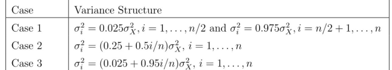
Case Variance Structure

Case 1 σ_i2 = 0.025σ_X2 , i= 1, . . . , n/2 and σ_i2 = 0.975σ2_X, i=n/2 + 1, . . . , n

Case 2 σ_i2 = (0.25 + 0.5i/n)σ2_X,i= 1, . . . , n

Case 3 σ_i2 = (0.025 + 0.95i/n)σ_X2, i= 1, . . . , n

Table 2.2: Three measurement error variance structures used in simulations.

Replicates X Case 1 Case 2 Case 3

No replicate X ∼χ2 3/ p (6) 1.277 (0.023) 1.030 (0.005) 1.113 (0.002) X ∼ Mixture 1 1.303 (0.022) 1.027 (0.006) 1.117 (0.012) X ∼ Mixture 2 1.109 (0.019) 1.011 (0.006) 1.039 (0.012) 2 replicates X ∼χ2 3/ p (6) 1.139 (0.018) 0.925 (0.014) 0.978 (0.015) X ∼ Mixture 1 1.005 (0.004) 0.992 (0.005) 0.998 (0.004) X ∼ Mixture 2 1.007 (0.002) 1.001 (0.003) 1.002 (0.002) 3 replicates X ∼χ2 3/ p (6) 1.150 (0.020) 0.965 (0.014) 1.034 (0.016) X ∼ Mixture 1 1.001 (0.004) 0.994 (0.004) 0.998 (0.004) X ∼ Mixture 2 1.008 (0.002) 0.999 (0.002) 1.002 (0.002) Table 2.3: The effect of the error variance structure on the ratio MISEeq/MISEopt and

the corresponding jackknife standard error (in parentheses) based on 1000 samples of size

n= 1000.

estimator compared to the EPF estimator.

Next, the effect of different underlying measurement error variance structures on the MISE ratio of the EPF and WEPFopt was examined. The sample size was fixed at

n = 1000 and the three different measurement error variance structures considered are outlined in Table 2.2. The ratios MSEeq/MSEopt based on 1000 simulated datasets are

reported in Table 2.3. Again, jackknife estimates of standard error are also reported. Inspection of Table 2.3 illustrates the effect of different heterogeneity patterns of mea-surement error variances on the performance of the EPF and WEPFopt estimators. When

the measurement error variances are known (J = 1), the WEPFopthas a lower MISE than

the EPF in all the considered configurations, with the heterogeneity pattern only affect-ing the size of the improvement. In the case of J = 2 replicates per observation, there were four instances in Case 2 and Case 3 of measurement error variances where the EPF performed better than the WEPFopt. This occurrence was likely because the estimated

weights for WEPFopt were calculated from estimated variance components based on only

J = 3, measurement error variances are estimated with higher accuracy, so the MISE ratio increase in general. Note that, although using WEPFopt can sometimes lead to a

worse performance, the loss tends to be small (at most 8% as seen in the Case 2 mea-surement error variance setting when X follows a Scaled-χ2

3 with 2 replicates); however, using WEPFoptcan still result in large gains (as much as 15% in the Case 1 measurement

error variance setting when X follows a Scaled-χ2₃ with 3 replicates).

In general, the simulation study shows that weighting to adjust for heteroscedasticity in estimating the phase function never results in a much poorer estimator, but sometimes leads to a large gain in efficiency. The loss/gain depends on how accurate measurement error variances were estimated as evidenced by the improvement in going from J = 2 to J = 3 replicates. In the next section, this is explored in the context of density deconvolution.

2.4. Density Estimation

2.4.1. Constructing an Estimator of fX

The outline here is a brief overview of how the method of Delaigle and Hall (2016) can be implemented using the WEPF to estimate the density function fX. Let ˆφW(t|q) and

ˆ

ρW(t|q) denote the weighted empirical characteristic function and corresponding WEPF

respectively. Let w(t) denote a non-negative weight function. Also let xj, j = 1, . . . , m

denote a set of arbitrary values with respective probability masses pj. Delaigle and Hall

(2016) suggest a two-stage estimation method for fX. First, one finds a characteristic

function of the form ψ(t|x,p) = P

jpjexp(itxj) that has phase function close to the

WEPF. Since this characteristic function corresponds to a discrete distribution with probability mass pj at the point xj for j = 1, . . . , m, the second stage of estimation

involves smoothingψ(t|x,p) before applying an inverse Fourier transformation to obtain the estimated density ˆfX(x). Delaigle and Hall (2016) suggest sampling thexj uniformly

on the interval [minWi, maxWi] with m= 5

√

that minimizes T(p) = Z ∞ −∞ ˆ ρW(t|q)− ψ(t|x,p) |ψ(t|x,p)| 2 w(t)dt (2.7) under the constraint of also minimizing the variance of the corresponding discrete dis-tribution, v(p) = Pm j=1pjx 2 j −( Pm j=1pjxj)

2_{. This non-convex optimization problem of} finding the solution{pˆj}mj=1 can be solved using MATLAB. Details are given in Delaigle and Hall (2016). The present implementation differs only in that the estimated phase function is weighted to adjust for heteroscedasticity. Beyond using a different estimator of the phase function, the optimization problem remains unchanged.

Now, let ψ(t|x,pˆ) = P

jpˆjexp(itxj) be the characteristic function with the ˆpjs the

probability masses estimated by minimizing (2.7). The deconvolution density estimator based on the WEPF is then

ˆ fX(x) = 1 2π Z exp (−itx) ˜φ(t)Kft(ht)dt (2.8) where ˜ φ(t) =        ψ(t|x,pˆ), fort ≤t∗ r(t), fort > t∗

with t∗ being the smallest t > 0 such that |φˆW(t|q)| < n−1/4. Here, Kft(t) denotes the

Fourier transform of a deconvolution kernel function and r(t) denotes a ridging func-tion. The ridging function ensures that the estimator is well-behaved outside the range [−t∗, t∗]. The proposed choice of ridging function isr(t) = ˆφW(t|q)/φˆL(t), with ˆφL(t) the

characteristic function of a Laplace distribution with variance equal to an estimator of

σ2

L=

P

jqjσ2j, the weighted sum of the measurement error variances. In application here,

the common choiceKft(t) = (1−t2)3 for|t| ≤1 is used. The weight function is chosen to be w(t) = ω(t)|φˆW(t|q)ψ(t|x,p)|2 with ω(t) = 0.75(1−t2) for|t| ≤1 (the Epanechnikov

kernel) rescaled to the interval [−t∗, t∗]. This choice of weight function avoids numerical difficulties that can arise when dividing by very small numbers.

2.4.2. Bandwidth Selection

The proposed phase function deconvolution estimator that accounts for heteroscedas-ticity in (2.8) is an approximation of the estimator

˜ f(x) = 1 2π Z exp (−itx)Kft(ht) ˆ φW(t|q) P jqjφεj(σjt) dt (2.9)

with ˆφW(t|q) defined in (2.2). Note that (2.9) is an estimator that one could compute

if the measurement error distribution were known, but that it is different from the het-eroscedastic estimator proposed by Delaigle and Meister (2008). Taking expectation of the integrated squared error (ISE) of (2.15), ISE = R

[ ˜f(x)− fX (x)]2dx, gives mean

integrated squared error (MISE)

MISE = 1 2π Z |φX(t)| 2 Kft(ht)−12dt+ 1 2π Z Kft(ht)2 P jq 2 j P jqjφεj(σjt) 2dt − 1 2π Z |φX(t)| 2 Kft(ht)2 P jq 2 jφ2εj(σjt) h P jqjφεj(σjt) i2dt. (2.10)

An argument similar to that of Delaigle and Meister (2008) when evaluating the asymp-totic MISE (AMISE) of their heteroscedastic estimator, one can show that the last term of (2.10) is negligible, giving AMISE = 1 2π Z |φX(t)| 2 Kft(ht)−12dt+ 1 2π Z Kft(ht)2 P jq 2 j h P jqjφεj(σjt) i2dt

In the present application, both φX(t) and φεj(t), j = 1, . . . , n are unknown. However, note that |φX(t)|2 =φX(t)φX (−t) is the characteristic function of the random variable

X −X0, where X, X0 are iid fX. Regardless of the shape of fX, the random variable

X−X0 is symmetric about 0 and has variance 2σ2

X. This suggests replacing|φX(t)|2 with

the characteristic function of a symmetric distribution with mean 0 and variance 2ˆσ2

X.

Appropriate choices might be the normal distribution, i.e. substituting exp (−σˆ2

Xt2) for

|φX(t)|

2

, or the Laplace distribution, i.e. substituting (1 + ˆσ2

Xt2)

−1

can use appropriate approximations for φεj(σjt). For example, the Laplace choice is a reasonable one, see Meister (2006) and Delaigle (2008). One can therefore substi-tute 1 + 0.5ˆσ2

jt2

−1

for φεj(σjt). This Normal-Laplace substitution gives approximate AMISE function ˆ A (h) = 1 2π Z      exp −σˆ_X2t2 Kft(ht)−12+ Kft(ht)2 P jq 2 j h P jqj 1 + 0.5ˆσj2t2 −1i2      dt (2.11)

and the value of h that minimizes the above function can then be used to evaluate the density deconvolution estimator in equation (2.8).

2.4.3. Simulation Study

Simulation studies were done to evaluate the performance of the equally-weighted and mean-optimal weighted phase function deconvolution density estimators. These corre-spond to the use of the EPF and WEPFopt as the phase function estimate before

per-forming the deconvolution operation as described in Section 2.4.1. Additionally, as it is already established in the literature, the Delaigle & Meister estimator, as proposed in Delaigle and Meister (2008) for heteroscedastic data, was also calculated. The three candidate distributions forX as described in Section 2.3.4 were considered. Both normal and Laplace distributions were considered for the measurement error, each in conjunction with the three measurement error variance models outlined in Table 2.2 being considered. In all cases the sample size was taken to be n = 500. Due to the computational cost of evaluating the phase function deconvolution estimators, a total of 500 samples were gen-erated for each combination ofX-distribution and variance model. For the phase-function estimators, the approximate AMISE bandwidth minimizing (2.11) was computed. The bandwidth of the Delaigle-Meister estimator was a two-stage plug-in bandwidth as sug-gested in their paper. For all the three deconvolution estimators, the integrated squared error (ISE) was computed for each sample.

mea-surement error variances are assumed known, and Table 2.5 presents the simulation results corresponding to the case with J = 2 replicates per observation and the variance com-ponents are estimated as outlined in Section 2.3.3. The simulation with replicate obser-vations contains results for the Delaigle-Meister estimator both using the estimated vari-ances (D&MVarE) and treating the variances as known (D&MVarK). Note that the simula-tions with replicate observasimula-tions use the individual-level average dataWi = (Wi1+Wi2)/2 to compute the deconvolution estimators and are therefore not directly comparable to the simulation without replication and measurement error variances assumed known. Due to the presence of outliers in the ISE calculations, the median as well as the first and third quartiles of 10×ISE are reported.

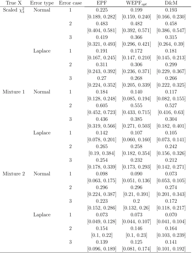
True X Error type Error case EPF WEPFopt D&M Scaledχ2 3 Normal 1 0.225 0.199 0.193 [0.189, 0.282] [0.159, 0.240] [0.166, 0.230] 2 0.483 0.482 0.458 [0.404, 0.581] [0.392, 0.571] [0.386, 0.547] 3 0.419 0.366 0.315 [0.321, 0.493] [0.296, 0.421] [0.264, 0.39] Laplace 1 0.191 0.172 0.181 [0.167, 0.245] [0.147, 0.210] [0.145, 0.213] 2 0.311 0.306 0.299 [0.243, 0.392] [0.236, 0.371] [0.229, 0.367] 3 0.27 0.268 0.266 [0.224, 0.352] [0.205, 0.339] [0.222, 0.325] Mixture 1 Normal 1 0.184 0.140 0.117 [0.128, 0.248] [0.085, 0.194] [0.082, 0.155] 2 0.605 0.555 0.527 [0.452, 0.723] [0.433, 0.715] [0.416, 0.63] 3 0.436 0.385 0.304 [0.319, 0.566] [0.271, 0.503] [0.182, 0.401] Laplace 1 0.142 0.107 0.105 [0.078, 0.201] [0.060, 0.160] [0.073, 0.141] 2 0.265 0.258 0.242 [0.19, 0.384] [0.182, 0.354] [0.156, 0.326] 3 0.254 0.232 0.212 [0.178, 0.339] [0.173, 0.293] [0.142, 0.271] Mixture 2 Normal 1 0.098 0.090 0.073 [0.063, 0.175] [0.051, 0.136] [0.053, 0.105] 2 0.296 0.296 0.274 [0.224, 0.387] [0.21, 0.391] [0.201, 0.343] 3 0.223 0.2 0.172 [0.152, 0.286] [0.132, 0.26] [0.118, 0.217] Laplace 1 0.073 0.073 0.070 [0.049, 0.128] [0.044, 0.107] [0.041, 0.104] 2 0.154 0.146 0.164 [0.1, 0.22] [0.1, 0.23] [0.103, 0.239] 3 0.139 0.125 0.141 [0.096, 0.189] [0.081, 0.174] [0.101, 0.192] Table 2.4: Density estimation for n = 500 with no replicates and measurement error variances are assumed to be known. The median, as well as first and third quartiles, [Q1, Q3], of 10 × ISE of density estimators under 500 simulations.

True X Error type Error case EPF WEPFopt D&MVarK D&MVarE Scaled χ2₃ Normal 1 0.204 0.192 0.178 0.274 [0.164, 0.259] [0.156, 0.241] [0.154, 0.205] [0.233, 0.319] 2 0.321 0.322 0.336 0.423 [0.252, 0.387] [0.267, 0.385] [0.28, 0.405] [0.384, 0.474] 3 0.29 0.285 0.249 0.384 [0.234, 0.327] [0.237, 0.33] [0.21, 0.298] [0.335, 0.419] Laplace 1 0.176 0.165 0.148 0.209 [0.142, 0.216] [0.140, 0.207] [0.123, 0.180] [0.176, 0.246] 2 0.277 0.273 0.281 0.343 [0.223, 0.349] [0.222, 0.337] [0.234, 0.338] [0.301, 0.378] 3 0.219 0.218 0.23 0.298 [0.18, 0.266] [0.176, 0.267] [0.184, 0.276] [0.249, 0.325] Mixture 1 Normal 1 0.128 0.120 0.097 0.206 [0.088, 0.182] [0.077, 0.166] [0.062, 0.145] [0.162, 0.277] 2 0.31 0.309 0.308 0.464 [0.214, 0.387] [0.217, 0.4] [0.232, 0.401] [0.404, 0.534] 3 0.257 0.242 0.195 0.374 [0.175, 0.345] [0.182, 0.339] [0.12, 0.266] [0.309, 0.451] Laplace 1 0.102 0.105 0.082 0.147 [0.066, 0.156] [0.074, 0.159] [0.058, 0.117] [0.106, 0.199] 2 0.216 0.21 0.223 0.308 [0.151, 0.271] [0.14, 0.267] [0.154, 0.272] [0.255, 0.355] 3 0.193 0.176 0.161 0.267 [0.13, 0.283] [0.119, 0.242] [0.114, 0.244] [0.229, 0.333] Mixture 2 Normal 1 0.081 0.084 0.064 0.123 [0.055, 0.111] [0.051, 0.110] [0.049, 0.088] [0.098, 0.150] 2 0.189 0.185 0.164 0.247 [0.112, 0.251] [0.118, 0.243] [0.126, 0.227] [0.204, 0.285] 3 0.132 0.125 0.118 0.201 [0.096, 0.193] [0.082, 0.194] [0.077, 0.144] [0.172, 0.239] Laplace 1 0.070 0.070 0.056 0.087 [0.049, 0.101] [0.046, 0.099] [0.037, 0.082] [0.059, 0.122] 2 0.136 0.117 0.15 0.181 [0.086, 0.187] [0.077, 0.163] [0.106, 0.186] [0.156, 0.214] 3 0.117 0.103 0.125 0.169 [0.076, 0.175] [0.073, 0.165] [0.086, 0.168] [0.138, 0.208]

Table 2.5: Density estimation forn = 500 withJ = 2 replicates for each observation. The median, as well as first and third quartiles, [Q1, Q3], of 10 × ISE of density estimators under 500 simulations.

Inspection of Table 2.4 reveals that the Delaigle-Meister (D&M) estimator tends to have the smallest median ISE, although there are a few instances in which the phase function estimators outperform the D&M estimator, notably for Mixture 2 and Laplace

measurement error. It is also clear that calculating the mean-optimal weights is very advantageous in this setting, with the mean-optimally weighted estimator having smaller median ISE than the equally weighted estimator in all but one instance. Overall, one can conclude that the WEPF estimator performs very well and compares favorably to the D&M estimator, the latter requiring knowledge of the measurement error distribution to be useful in practice.

Inspection of the simulation results in Table 2.5 is very insightful. Note that the measurement error variances here are estimated based on only J = 2 replicates for each observation. As such, one might not expect good performance. However, the two phase function estimators perform very favorable when compared to the D&M estimator with known measurement error variances. The mean-optimally weighted estimator generally performs better than the equally weighted estimators in terms of median ISE, although there are two exceptions. It is interesting that weights estimated based on only two repli-cates give such good performance. Also revealing is that the WEPF estimator performs significantly better than the D&M estimator with estimated variances, with the median ISE of the mean-optimally weighted estimator often reflecting more than a 50% reduction in median ISE when comapared to the D&M counterpart.

Figures 2.1 and 2.2 show plots of the density estimators corresponding to the first, second, and third quantiles (Q1, Q2, and Q3) of ISE for each of the methods EPF, WEPFopt, and the D&M estimators corresponding to X having scaled χ23 and Mixture 1 distribution. In all three instances, the estimators were calculated with estimated measurement error variances based on J = 2 replicates per observation. Observation-level measurement error was taken to be Case 1 of Table 2.2. Both normal and Laplace distributions were considered for the measurement error. The sample size was fixed at n = 500. The figures also show the true density curve for comparison. Although all three estimators considered are able to capture the shape of the true density, the D&M estimators with estimated variance do the worst among the three: ForX having a scaled χ2₃ distribution, it puts much more density in negative support than the EPF and WEPFopt and tends to underestimate the modal height. Both the EPF with WEPFopt,

perform well for the scaled χ2

3 distribution, with the WEPFopt seemingly capturing the

shape around the mode a little better than the EPF. When evaluating Figure 2.2 showing the same plots for X having the distribution Mixture 1, the general observations are very similar. The EPF and WEPFopt have visually similar performance, while the D&M

estimator underestimates the density around the mode. The Appendix 2.7.3 also contains a set of plots corresponding to X having Mixture 2 distribution. Similar observations apply there.

Additional simulation results are presented in the Appendix 2.7.3. There, the EPF, WEPF and D&M estimators are compared under the assumption that one can find an optimal bandwidth (a bandwidth minimizing ISE) for any observed sample. When no replicate data is available and the measurement error variances are assumed known, the D&M estimator has the best performance, and the WEPF outperforms the EPF in all but one case considered. However, once the measurement error variance needs to be estimated (for both J = 2 and J = 3 replicates per case), the WEPF estimator tends to have the best performance, with the D&M estimator faring worse than the EPF estimator. Finally, a simulation with plug-in bandwidth and J = 3 replicates is also presented. Here, the EPF and WEPF both outperform the D&M estimator.

2.5. Analysis of Framingham Data

In this section, the EPF and WEPFoptdensity deconvolution estimators are illustrated

using a classical dataset in the deconvolution literature, a subset of the Framingham Heart Study. The data consists of several variables related to coronary heart disease for n = 1615 patients. For each patient, two measurements of long-term systolic blood pressure (SBP) were collected at each of two examination. As per Carroll et al., Carroll et al. (2006) let Mij be the average of the two measurements at exam j for j = 1,2,

and let Wij = log(Mij − 50). The Wij are assumed to be related to true long-term

SBP, Xi according to Wij =Yi +σiεij with Yi = log(Xi−50). Density deconvolution is

therefore used to estimate the density on the Y-scale, ˆfY(y), after which it follows that

ˆ

−1 0 1 2 3 4 5 6 0.0 0.2 0.4 0.6 0.8 Plug−in x density −1 0 1 2 3 4 5 6 0.0 0.2 0.4 0.6 0.8 Plug−in x density −1 0 1 2 3 4 5 6 0.0 0.2 0.4 0.6 0.8 Plug−in x density (a) (b) (c) −1 0 1 2 3 4 5 6 0.0 0.2 0.4 0.6 0.8 Plug−in x density −1 0 1 2 3 4 5 6 0.0 0.2 0.4 0.6 0.8 Plug−in x density −1 0 1 2 3 4 5 6 0.0 0.2 0.4 0.6 0.8 Plug−in x density (d) (e) (f ) Figure 2.1 : Curv es Q1 ( ), Q2 ( ), Q3 ( ), and true curv e ( ) for X ∼ Scaled-χ 2 ,3 n = 500, J = 2 replicat es p er observ a tion when the errors are Normal (a )-(c), and Laplace (d)-(f ), with case 1 of measuremen t error v ariances. F or (a),(d): EPF estimator; (b),(e): WEPF opt estimator; (c),(f ): D&M estimator with estimated v ariances. All estimators are computed using plug-in bandwidth discussed in Section 2.4.2.

−2 0 2 4 6 0.0 0.2 0.4 0.6 0.8 Plug−in x density −2 0 2 4 6 0.0 0.2 0.4 0.6 0.8 Plug−in x density −2 0 2 4 6 0.0 0.2 0.4 0.6 0.8 Plug−in x density (a) (b) (c) −2 0 2 4 6 0.0 0.2 0.4 0.6 0.8 Plug−in x density −2 0 2 4 6 0.0 0.2 0.4 0.6 0.8 Plug−in x density −2 0 2 4 6 0.0 0.2 0.4 0.6 0.8 Plug−in x density (d) (e) (f ) Figure 2.2 : Curv es Q1 ( ), Q2 ( ), Q3 ( ), and true curv e ( ) for X ∼ Mixture 1, n = 500, J = 2 replicates p er observ ation, when the errors are Normal (a)-(c), and Laplace (d)-(f ), with case 1 of measuremen t error v ariances. F or (a),(d): EPF estimator; (b),(e): WEPF opt estimator; (c),(f ): D&M estimator with estimated v ariances. All estimators are computed using plug-in bandwidth discussed in Section 2.4.2.

For the SBP data, the EPF and WEPFopt were estimated, the latter with

mean-optimal weights qopt using variance components estimated as described in Section 2.3.3.

For both the EPF and WEPFopt, deconvolution bandwidths were estimated using (2.11).

These two estimators are shown in Figure 2.3, together with the Delaigle & Meister (2008) estimator using the same estimated variances and Laplace measurement error. (The D&M estimator was also calculated for normal measurement error and was nearly identical.) A naive kernel estimator of the data using a normal references bandwidth is also shown for comparative purposes. Other bandwidth selection approaches for the naive kernel estimator were also considered with very similar results. The naive kernel estimator is much flatter around the mode and fatter in the tails. This is expected, as the kernel estimator makes no correction for the measurement error present in the data. Furthermore, it can be seen that the WEPFopt and EPF deconvolution density

estimators are similar. The two density estimators based on phase functions suggest that the distribution of X may be multi-modal, while the D&M estimator is unimodal and positive skew. 80 100 120 140 160 180 200 0 0.005 0.01 0.015 0.02 0.025 0.03 0.035 _Naive EPF WEPF opt Laplace ME

Figure 2.3: Estimation of the densityfX in the Framingham data. Four density estimates

are shown: a naive kernel estimator (measurement error is ignored), the EPF estimator, the WEPFopt estimator, and the Delaigle & Meister estimator assuming Laplace

2.6. Conclusions

This chapter presents a method for phase density deconvolution with heteroscedas-tic measurement error of unknown type and builds on the work of Delaigle and Hall (2016) who considered the homoscedastic case. Two estimators are proposed, one us-ing equally weighted observations and the other usus-ing mean-optimal weights to adjust for heteroscedasticity of the measurement error. A method based on approximating the AMISE is proposed for bandwidth selection in both instances. In the simulation settings considered, the WEPFopt estimator generally performed better than the EPF estimator,

although there were instances where their performance was comparable. The simula-tion results suggest that mean-optimal weighting of observasimula-tions will not have a detri-mental effect on estimating the density function, and big gains are sometimes possible. The practitioner cautious about estimaging weights from a small number of replicates could always opt for a hybrid type of estimator, calculating WEPFhybrid using weights qhybrid=αqopt+ (1−α)/n whereα indicates their degree of confidence in using the esti-mated weights. The performance of this hybrid estimator is a future avenue of research. In the setting where the measurement error variances are known, the method of Delaigle and Meister (2008) will outperform both phase function estimators, although the latter are still competitive in this setting. Also recall that the Delaigle & Meister estimator requires knowledge of the measurement error distribution — an assumption not made by the EPF and WEPF estimators. When there are only 2 replicates per individual from which to estimate the measurement error variances, the phase function methods performed substantially better than the Delaigle & Meister estimator. This suggests that the phase function methods have some inherent robustness against variance estimate de-viation from the true values, and that the phase function density estimators can generally do the same as Delaigle & Meister estimator with much less assumption on measurement error.

2.7. Appendix

2.7.1. Asymptotic Properties of the Weighted Empirical Phase Function (WEPF)

Assume the observed data are of the form Wi = Xi+σiεi, where the Xi are an iid

sample from fX, the measurement error terms εi are independent of one another and

of the Xi, and each εi has a symmetric distribution with strictly positive characteristic

function and satisfies E(εi) = 0 and Var(εi) = 1. The σi are non-negative constants

that account for measurement error heteroscedasticity. For any random variable Z and a complex number z, denote φZ(t) as the characteristic function of a random variable

Z and |z| = (zz¯)1/2 _{as the norm function with ¯z the complex conjugate of z. Define a} weighted empirical characteristic function for the Wi,

ˆ φW(t|q) = n X j=1 qjexp(itWj) (2.12)

whereq={q1, . . . , qn}denotes a set of non-negative constants that sum to 1. Let ˆψW(t|q)

denote the squared norm of that function,

ˆ ψW(t|q) = X j X k qjqkexp [it(Wj −Wk)].

The WEPF is defined as

ˆ ρW(t|q) = ˆ φW(t|q) ˆ ψ_W1/2(t|q). (2.13) The asymptotic properties of the WEPF are given in Theorem 2.1, which is restated here for completeness.

Theorem 2.1. Assume that maxjqj =O(n−1) and that each measurement error

compo-nent εj has a strictly positive characteristic function. It then follows that the WEPF as