A Quantitative Assessment of the Decline in the U.S. Saving
Rate and the Current Account Balance
Kaiji Cheny Ay¸se ·Imrohoro¼gluz Selahattin ·Imrohoro¼gluz
First Version October 2005; this Version April 2008
Abstract
We use the standard growth theory to evaluate the quantitative role of changes in the population growth rate, depreciation rate, tax rate on capital and labor income, and the TFP growth rate in explaining the decline in the saving rate and the current account balance in the U.S. Our …ndings suggest that the decline in the population growth rate and the increase in the depreciation rate play a signi…cant role in explaining the secular trends in the U.S. saving rate up to early 1990s. We also …nd that the model is capable of capturing the current account de…cit between the U.S. and the OECD countires, thus explaining one third of the overall U.S. current account de…cit. Our results indicate that di¤erences in the TFP growth rates between U.S. and it’s trading partners may have been responsible for the secular decline in the U.S. current account.
Department of Economics, University of Oslo
zDepartment of Finance and Business Economics, Marshall School of Business,
Uni-versity of Southern California, Los Angeles, CA 90089-1427.
We would like to thank the seminar participants at USC, University of California at Riverside, Federal Reserve Bank of Chicago, Conference on Economic Dynamics at the University of Tokyo, 2006 Annual Meet-ings of the Society for Economic Dynamics, CEMFI, Madrid, IIES, Stockholm University, Indiana University, Purdue University, CERGE-EI, Charles University in Prague and University of Iowa for helpful comments.
1
Introduction
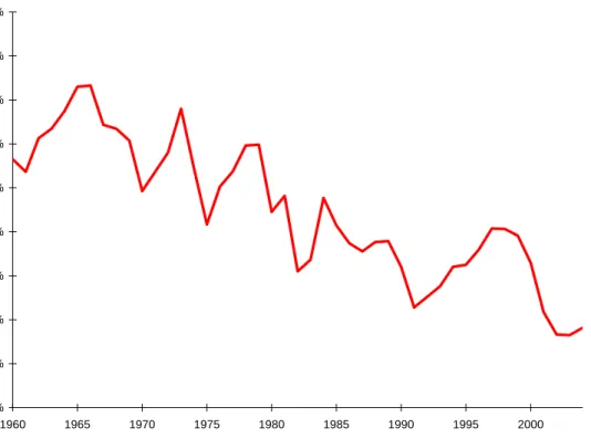
The net national saving rate in the U.S., displayed in Figure 1, has declined from an average of 15% in 1960s to 10% in 1980s and 8.6% in 1990s. This secular decline has occupied center stage in policy discussions and continues to attract media coverage. Understanding this decline as well as the di¤erences in saving rates across countries have been an important part of academic research. Detailed analyses have been conducted to explore whether particular birth cohorts are responsible for the low saving rate by examining personal saving rates in the U.S. For example, Gokhale, Kotliko¤, and Sabelhaus (1996) attribute the decline in the saving rate to the redistribution of resources through social security and medicare, from young consumers with low marginal propensities to consume, to older generations with high marginal propensities to consume. Attanasio (1998) argues that cohorts born between 1925 and 1939 may be to blame for the low personal saving rate. Summers and Carroll (1987) suggest that it is the reliance of the younger generations on social security that depresses saving in the U.S. Boskin and Lau (1988a,b) formulate a model based on longitudinal and cross-sectional microeconomic data together with aggregate time series and examine the importance of various factors a¤ecting aggregate consumption and saving in the U.S. Their results suggest that it is the decline in the saving of generations born after the great depression that may be responsible for the decline in the national saving rate.1
Another notable change between 1960 and 2004 has been the growing current account (CA) de…cit in the U.S. Figure 2 displays the CA de…cit between the U.S. and a set of its trading partners during this time period. The secular decline in the current account especially since the 1990s is evident in all the series.2 Several authors have been analyzing the consequences of these large global imbalances. There seem to be two opposing views on this issue. On the one hand there is growing concern about the consequences of these global imbalances. For example, Obstfeld and Rogo¤ (2004) predict that the current account imbalances in the U.S. will result in a 30% depreciation of the dollar. Roubini and Setser (2005) suggest that the U.S. is on an unsustainable and dangerous path. Summers (2004) cautions that the current account de…cit in the U.S. has all the hallmarks of a particularly
1
Another set of papers have focused on the possible relationship between the increase in stock prices and the boom in consumer spending. For example, Parker (1999) and Juster, Lupton, Smith, and Sta¤ord (2000) suggest that the signi…cant capital gains in corporate equities experienced since 1984 are responsible for the more recent decline in the personal saving rate. Backus, Henriksen, Lambert, and Telmer (2005) argue that private saving rates are strongly and negatively correlated with the ratio of net worth to consumption. Also see Poterba (2000) for a survey.
2
Data on U.S. current account balance against various regions come from International Economic Accounts of Bureau of Economic. The data on the U.S. current account balance against our sample of OECD countries are the sum of the U.S. current account balances against Western Europe, Canada and Japan. After 1998 we use the U.S. current account balance against EU-15 to substitute for U.S. current account balance against Western Europe. Bilateral current account balance between U.S. and China is available since 1997.
2% 4% 6% 8% 10% 12% 14% 16% 18% 20% 1960 1965 1970 1975 1980 1985 1990 1995 2000 Saving Rate
Figure 1: Net National Saving Rate in the U.S.
serious situation. On the other hand, in a descriptive paper, Backus, Henriksen, Lambert and Telmer (2005) suggest that the current account de…cit in the U.S. is mainly due to the weak economic conditions in several high-surplus countries relative to the U.S. and argue that “things are …ne”. Several other explanations have been put forward to try to understand potential causes of the current account de…cit. Fogli and Perri (2006) argue that the fall in the U.S. business cycle volatility has lead to lower precautionary savings resulting in lower current account balances. Mendoza, Quadrini and Rios-Rull (2007) argue that the U.S. has been accumulate foreign liabilities because the …nancial markets in the rest of the world are less well developed. Finally, Attanasio and Violante (2005), Domeij and Floden (2006), Henriksen (2005), and Krueger and Ludwig (2006) highlight the importance of demographic di¤erences between regions leading to large and persistent current account imbalances.
Since 1960s there have been substantial changes in several macroeconomic indicators in the U.S. and the rest of the world that can have important consequences for the behavior of the national saving rates and the current account balances. For example, the average population growth rate and the depreciation rate between 1960 and 1980 in the U.S. were 1.8% and 4.3%, respectively. By 2000 the population growth rate had declined to about 0% while the depreciation rate had increased to 5.3%. While both of these changes would put a downward pressure on the saving rate in the U.S., there were other changes in the
CA Balance/GDP -6% -5% -4% -3% -2% -1% 0% 1% 2% 1960 1965 1970 1975 1980 1985 1990 1995 2000 2005 Total CA balance/GDP OECD Sum-China
Figure 2: U.S. Current Account De…cit
economic environment, such as the decline in the capital income tax rate, that would have encouraged savings over this time period. Meanwhile some of these exogenous variables have been changing at di¤erent rates in the rest of the world. In particular, we later document that the rates of growth of total factor productivity (TFP) in a set of OECD countries relative to the U.S. have declined between 1960 and 2004.
In this paper we explore the quantitative implications of changes in TFP growth rates, factor income tax rates, population growth rates and depreciation rates in the U.S. relative to its trading partners on the secular trends in the net national saving rate and the current account balance using the standard growth theory.3 We start by studying the U.S. as a closed economy. We employ the neoclassical growth model with an in…nitely-lived repre-sentative agent facing complete markets. We calibrate the economy to the U.S. data for the 1960-2004 period and use this model to isolate the quantitative impact of the domestic factors on the decline in the U.S. saving rate. First we show that the simple growth model is able to capture the consumption-saving trade-o¤ reasonably well. Next, we conduct
deter-3
Our approach is in line with the recent use of the one-sector growth model to explain ‘Great Depressions’. In particular, we follow the methodology of Cole and Ohanian (1999, 2002, 2004), Kehoe and Prescott (2002), and Chen, ·Imrohoro¼glu and ·Imrohoro¼glu (2006) in using an applied general equilibrium setup to account for the observed time path of the U.S. saving behavior and the current account balance.
ministic simulations, as in Hayashi and Prescott (2002), and perform an accounting exercise to evaluate the quantitative impact of the population growth rate, depreciation rate, TFP growth rate, and tax rates on the secular trends in the U.S. saving rate. Our results suggest that the secular decline in the population growth rate and the increase in the deprecation rate explain nearly half of the decline in the net national saving rate in the U.S. Changes in the TFP growth rate generate annual ‡uctuations in the saving rate that resemble the data reasonably well.
In order to address the decline in the U.S. saving rate and the CA balance simultaneously, we specify a two country economy where di¤erences between the U.S. and the rest of the world (ROW) with respect to the exogenous variables are introduced. For the ROW we restrict our attention to a subset of OECD countries for which we have consistent measurements. We calibrate their TFP growth rates, population growth rates, shares of government purchases in output, and tax rates on capital and labor income for the same period. Overall our results indicate that it is possible to generate realistic current account de…cits for the U.S. in a carefully calibrated model. We conduct several counterfactual experiments to investigate the factors behind the secular decline in the U.S. current account. Our …ndings indicate that di¤erences in the TFP growth rates play a signi…cant role in the secular decline of the U.S. current account. We show that if the only di¤erence between the U.S. and the ROW were their TFP growth rates, the model would still generate a declining current account balance for the U.S. When the TFP growth rates are relatively higher in the U.S., so are the returns to capital in the U.S. This drives up the demand for investment in the U.S. relative to its trading partners and its own domestic saving, generating the main reason for the secular increase in the current account de…cit in the model economy.
Although the simple growth model is useful in explain some of the features of the U.S. saving rate and the current account balance, signi…cant puzzles remain. In particular, the model misses the U.S. boom in hours in the 1990s. Consequently, the model generated NIPA accounts miss their empirical counterparts after 1990s as others have also demonstrated.4 Once a labor wedge, as in Chari, Kehoe and McGrattan (2004) or Ohanian, Ra¤o, and Rogerson (2006) is incorporated into the model the match improves signi…cantly. Neverthe-less, we argue that the model captures the consumption-saving trade-o¤ reasonably well and can be a useful tool in understanding the main factors impacting the secular behavior of savings and current account balances.
The paper is organized as follows. Section 2 presents the growth model used in the paper and how it is calibrated to the U.S. economy. Our main quantitative …ndings are presented in Section 3. The results of the extension of the model to a two-country economy are given in Section 4. Section 5 conducts a sensitivity analysis and concluding remarks are given in Section 6. The Appendix contains calibration details and data sources.
2
The Standard Growth Model
In this section we examine the properties of an closed economy. This allows us to isolate the quantitative impact of the domestic factors on the decline in the U.S. saving rate between 1960 and 2004. We show that the standard neoclassical model can be an e¤ective tool in understanding the behavior of the saving rate until the early 1990s. In the next section we examine an open economy where di¤erences between the U.S. and the ROW with respect to the exogenous variables are introduced. We investigate the role of these exogenous variables in impacting the secular movements in the U.S. current account.
2.1 The Environment
There is a stand-in household with Nt working-age members at date t, that solves
max 1 X t=0 tN t(logct+ log(1 ht)) subject to Ct+Xt (1 h;t)wtHt+rtKt k;t(rt t)Kt+T Rt t;
where ct =Ct=Nt is per member consumption, ht= Ht=Nt is the fraction of hours worked
per member of the household, is the subjective discount factor, is the share of leisure in the utility function, Htis total hours worked by all working-age members of the household, h;t and k;t are tax rates on labor and capital income, respectively, at timet; wtis the real
wage,T Rtis a government transfer, tis a lump sum tax,rtis the rental rate of capital, and t is the time-tdepreciation rate. The size of the household evolves over time exogenously
at the rate nt = Nt=Nt 1: Households are assumed to own the capital, Kt; and rent it to
businesses.
The economy-wide resource constraint is given by
Ct+Xt+Gt=Yt;
where aggregate consumption, investment and government purchases add up to aggregate output. The law of motion for the capital stock is given by Kt+1 = (1 t)Kt+Xt:
The aggregate production function is given by
Yt=AtKt(Ht)1 ;
where is the income share of capital and At is total factor productivity, which grows
exogenously at the rate gt=At=At 1.
There is a government that taxes income from labor and capital (net of depreciation) and uses the proceeds to …nance exogenous streams of government purchasesGtand government
transfers T Rt:A lump sum tax t is used to ensure that the government budget constraint
is satis…ed each period:
Gt+T Rt= h;twHt+ k;t(rt t)Kt+ t:
In other words, t is the primary government de…cit in the model.
The de…nition of the competitive equilibrium of this economy is standard and provided in the Appendix 7.1.
2.2 Measurement and Calibration
We measure the saving rate using
st=
Yt Gt Ct tKt Yt tKt
:
where in this closed economy Ytis measured using GNP.
We calibrate the model economy using data from the 2005 revision of National Income and Product Accounts (NIPA), Fixed Asset Tables (FAT) of Bureau of Economic Analysis (BEA), Statistics of Income (SOI), Individual Income Tax Returns (1960-2003), and the Social Security Bulletin.
Constant Parameters: There are 3 parameters that are time invariant throughout our analysis. The capital share parameter, ; is set to its average value of0:4 over our sample period 1960-2004. The subjective discount factor, ; is set to 0:9702 so that the capital output ratio is 3:2 at the …nal steady state. The share of leisure in the utility function, ;is set to 1:45 to match an average workweek of 35 hours.
Calibration of the 1960-2004 period: In our benchmark simulation, we use the actual time series data between 1960-2004 for the following exogenous variables: TFP growth rate,
gt 1; population growth rate, gt 1; depreciation rate, share of government purchases in
GNP, t;share of government transfers in GNP,T Rt=GN Pt;and capital and labor income
tax rates, k;t; h;t.5 Empirical marginal tax rates are constructed using the methods of
Joines (1981) and McGrattan (1994). The data used in the calibration are provided in the
5
T F P is calculated as
At=Yt=Kt(Ht)
1
;
where the capital share is set to 0:4, Yt is GN P plus service ‡ow from the stock of consumer durables and government capital, Kt is capital stock inclusive of foreign capital, stock of consumer durables and government capital, andHtis aggregate hours worked. In this framework savings consists of domestic private investment and the current account surplus. Even though we treat the model as a closed economy, we include the foreign capital in the de…nition of the capital stock to make sure that the TFP growth rates faced by the U.S. individuals can be accurately measured. However, it is important to note that this adjustment is quantitatively very small. None of the results are signi…cantly altered by di¤erent measurements of TFP such as inclusion of government capital or the exclusion of foreign capital. Several TFP growth rates based on di¤erent de…nitions of capital are provided in the Appendix 7.6. Gomme and Rupert (2005) also provide
Appendix 7.2. We compute the initial capital-output ratio in 1960 as 3:5 and take it as a given initial condition.
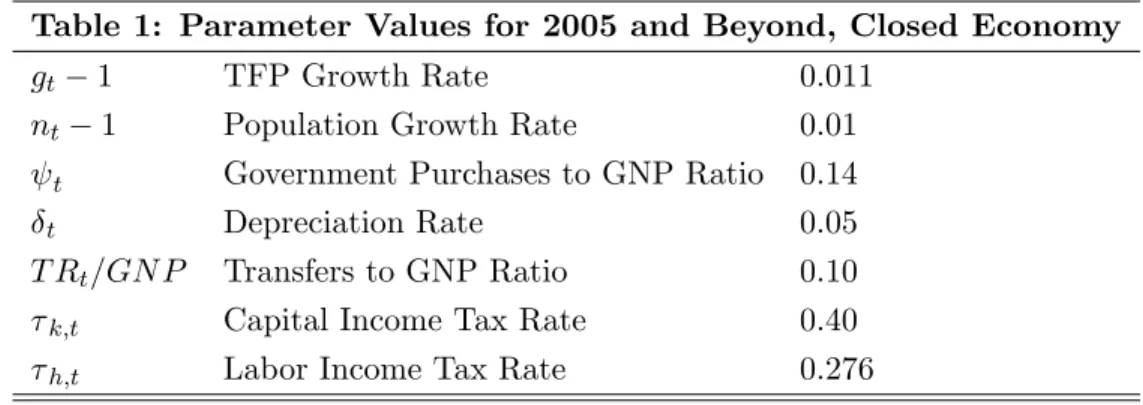
Calibration of 2005 and beyond: We assume that the U.S. economy starts from given conditions in 1960 and eventually converges to a steady-state in 2070.6 In our benchmark model, we set the exogenous variables listed in table 1 equal to their steady state values starting in 2005.7 Note that the population growth rate in the U.S. has been declining since the 1960s and according to the Census Bureau projections it will continue at very low rates in the future. Based on the ‘middle’ growth projections by the Census Bureau’s we set the population growth rate after 2004 and at the steady state equal to 1%:8 Similarly, the depreciation rate has been increasing in the U.S. For the periods after 2004 and at the steady state, we set the depreciation rate equal to5%which is the depreciation rate in 2004.9 Our results are not sensitive to di¤erent assumptions about the calibration of most of the variables for the period 2005 and beyond. One variable that matters for the results is the growth rate of TFP. We discuss its impact in the sensitivity analysis.
Table 1: Parameter Values for 2005 and Beyond, Closed Economy
gt 1 TFP Growth Rate 0.011
nt 1 Population Growth Rate 0.01 t Government Purchases to GNP Ratio 0.14
t Depreciation Rate 0.05
T Rt=GN P Transfers to GNP Ratio 0.10
k;t Capital Income Tax Rate 0.40 h;t Labor Income Tax Rate 0.276
three di¤erent measures of the U.S. TFP growth rate based on very di¤erent assumptions on the capital stock. The TFP growth rates implied by their results as well as ours display very similar properties over this time period.
6
This is an approximation. Allowing for a longer transition period from 1960 for convergence to a steady-state has no quantitative impact on the 1960-2004 period we are investigating.
7
With our assumed tax rates, the government budget will be in a surplus at the steady state. 8
Population growth rates are the growth rates of civilian non-institutional population 16 years and over reported by the BLS. Population projections are taken from U.S. Bureau of the Census (http://www.mnforsustain.org/united_states_population_growth_graph.htm)
9Gomme and Rupert (2005) provide detailed calculations for the depreciation rate of di¤erent types of capital. Increasing depreciation rates are evident in computers and to some extent in market structures since 1960s.
2.3 Numerical Solution
Our numerical solution procedure follows Hayashi and Prescott (2002). After calibrating the model parameters and exogenous variables, we …rst compute a …nal steady-state for the U.S. economy in a su¢ ciently distant future. To obtain this steady-state, we derive the equilibrium conditions of the model, detrend variables to induce stationarity, and then impose these steady-state conditions.10 Given this …nal steady-state, we use a shooting algorithm from given initial conditions in 1960 toward the …nal steady-state to compute the transition path. In particular, we start from a given value of the initial capital stock K0;guess a value
for the endogenous variableC0 and use the Euler equation and resource constraint to obtain
a path for the endogenous variables Ct, Ht and Kt+1 towards their steady-state values. If
the path does not connect with the steady-state, we iterate on the initial guess for C0 using
this ‘shooting’ algorithm until convergence to the steady-state is obtained. Equipped with the equilibrium path of Ct; Ht and Kt+1;we can then use other equilibrium conditions to
construct time paths of all aggregate quantities and prices.
3
Results for the Closed Economy
In this section we will …rst examine the general properties of the neoclassical growth model. Next, we will examine its implications for the U.S. saving rates.
3.1 General Properties
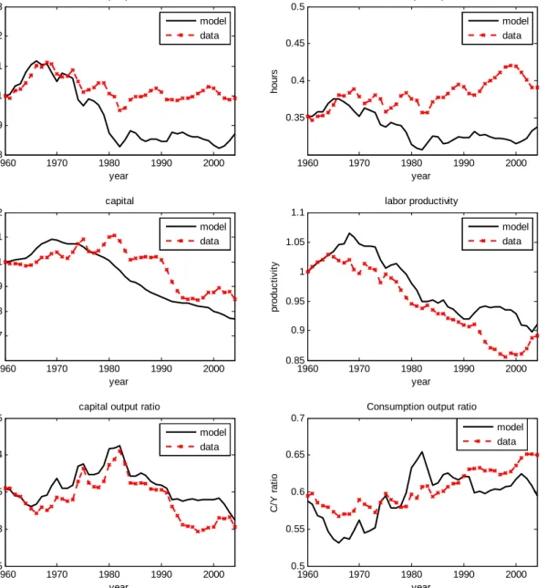
Figure 3 displays the model’s predictions for per capita GNP, hours, capital, labor produc-tivity, capital output ratio and consumption output ratio together with their counterparts in the data. The model generated series and the data, except for hours per capita, are all detrended by 1.018t.
The model generated per capita hours and GNP display large gaps from their data counterparts, as shown in Figure 3. In particular, simulated labor supply displays a decline while hours per capita in the data increase.11 As a result, we observe a divergence of our theory from data for both average labor productivity and capital-output ratio from early 1990s, although the discrepancy between the model and data is relatively small before then. The reason for the hours boom in the U.S. is not well established. One possibility is the increase in the labor force participation of women. McGrattan and Rogerson (2004) show that the increase in hours per capita observed in the U.S. is mainly due to the increase in the labor force participation rate of females. In fact, between 1950 and 2000, employment to population ratio of women increases by 87% while that of men declines by 15.7%. Between
1 0
The details are provided in the Appendix 7.1. 1 1
1960 1970 1980 1990 2000 0.8 0.9 1 1.1 1.2 1.3 GNP per person year GNP per pers on 1960 1970 1980 1990 2000 0.35 0.4 0.45 0.5
hours per capita
year hours 1960 1970 1980 1990 2000 0.7 0.8 0.9 1 1.1 1.2 capital year c api tal 1960 1970 1980 1990 2000 0.85 0.9 0.95 1 1.05 1.1 labor productivity year produc ti v it y 1960 1970 1980 1990 2000 2.5 3 3.5 4 4.5
capital output ratio
year K/Y r a ti o 1960 1970 1980 1990 2000 0.5 0.55 0.6 0.65 0.7
Consumption output ratio
year C /Y r a ti o model data model data model data model data model data model data
1980 and 2000 employment to population ratio of women increases by 17%. The simple framework used in this model is not capable of mimicking these trends.12 It is also possible that the reason for the hours boom lies somewhere else such as the intangible capital expla-nation advanced by McGrattan and Prescott (2007a) or the change in wage markups argued by Smets and Wouters (2007).
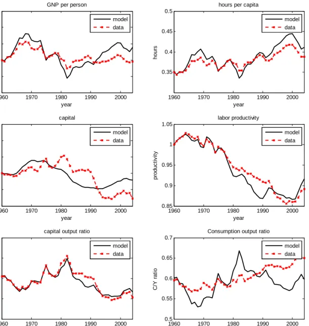
In order to further understand the performance of the standard model, but without taking a stand on the main reasons behind the hours boom in the data, we introduce a labor wedge into the model. We would get a perfect match between the model and the data if we introduced a labor wedge and an investment wedge that would force equations 13 and 15 to hold. In the following experiment we introduce only the labor wedge to examine the role of labor in generating the results in Figure 3. Speci…cally we use the labor wedge calculated from
Lwt=
htCt
(1 ht)(1 h;t)(1 )Yt :
After computing the labor wedge we replace (1 h;t) in equation 13 with (1 h;t)Lwt:
Since we already have taxes in this model, the labor wedge would have to be a proxy for labor distortions other than taxes.
Figure 4 displays the results of this experiment with the labor wedge. Hours per capita do not match the data perfectly since we only have the labor wedge and do not have the investment wedge. The rest of the model-generated series resemble the U.S. data reasonably well. In particular, after we use labor wedges to generate an hours boom in the 1990s, the model accounts for both average labor productivity and capital-output ratio reasonably well. We conjecture that extensions of the standard model which can capture the hours boom may be successful in mimicking the other aspects of the U.S. economy well.13
3.2 Consumption-Output Ratio, Saving Rate and Interest Rate
We now turn our focus to the consumption-output ratio and the saving rate to evaluate the extent to which the model is able to mimic the real interest rate and the consumption-saving trade-o¤. In order to quantify this trade-o¤, it will be useful to re-write the Euler equation as Ct+1=Yt+1 Ct=Yt = Yt Yt+1 [1 + (1 k;t+1) (rt+1 t+1)]: (1) 1 2
Several papers investigate the rise of the female labor force participation such as Jones, Manuelli and McGrattan (2003), Olivetti (2001), Akbulut (2005), and Caucutt, Guner, and Knowles (2002).
1 3The labor wedge needed to generate these results is not non-negligible especially for the 1984-2004 period. It starts at the value of 1.0 in 1960 and grows to 1.12 at the end of 1984. However, the wedge that is needed to match the hours has to increase by 42% between 1984 and 2004. It is hard to explain the size of the wedge using labor distortions other than taxes especially for the later period. For the earlier period, it is possible that a model which incorporates the increases in labor force participation of women may explain the size of the wedge needed.
1960 1970 1980 1990 2000 0.8 0.9 1 1.1 1.2 1.3 GNP per person year GNP per pers on 1960 1970 1980 1990 2000 0.35 0.4 0.45 0.5
hours per capita
year hours 1960 1970 1980 1990 2000 0.8 0.9 1 1.1 1.2 1.3 capital year c api tal 1960 1970 1980 1990 2000 0.85 0.9 0.95 1 1.05 labor productivity year produc ti v it y 1960 1970 1980 1990 2000 2.5 3 3.5 4 4.5
capital output ratio
year K/Y r a ti o 1960 1970 1980 1990 2000 0.5 0.55 0.6 0.65 0.7
Consumption output ratio
year C /Y r a ti o model data model data model data model data model data model data
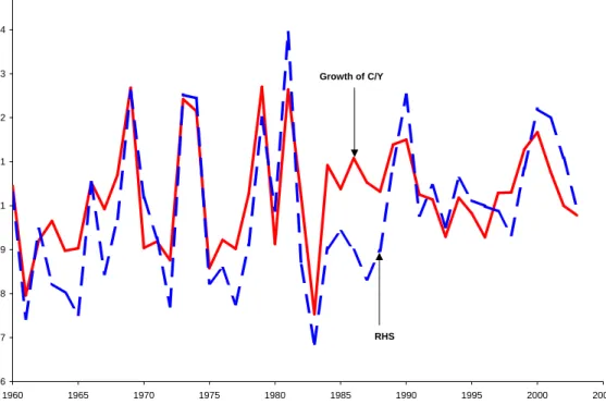
0.96 0.97 0.98 0.99 1 1.01 1.02 1.03 1.04 1.05 1960 1965 1970 1975 1980 1985 1990 1995 2000 2005 Growth of C/Y RHS
Figure 5: Investment Wedge
The left hand side of (1)is the growth rate of consumption-output ratio, which we can easily calculate from NIPA (after reorganizing the accounts so they match model accounts). We can also calculate the model-generated growth rate of consumption-output ratio using the right hand side of (1), takingYt andrt from the data. We call the discrepancy between
the the two computations the “investment wedge”.
Figure (5) plots the rate of growth of consumption-output ratio from the data (the LHS of (1)) and the model’s prediction for the same growth rate after using the data on output and the real interest rate. We observe that the two measures for the growth rate of consumption-output ratio track each other very closely except the brief period in the mid- to late-1980s. This indicates that the standard theory is able to capture the consumption-saving trade o¤ fairly well without the need to introduce additional frictions.
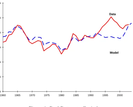
How well does the model perform in terms of the real interest rate? Figure (6) displays the after-tax rate of return to capital in the data and the model economy. We see that the model-generated after-tax rate of return to capital is fairly close to the data except for the mid- to late-1990s. Note that this divergence between the model and data in the 1990s is closely linked to the failure of our model to generate the hours boom in that period. In our model, hours are depressed in the 1990s while in the data they are booming. As a result,
1% 2% 3% 4% 5% 6% 7% 1960 1965 1970 1975 1980 1985 1990 1995 2000 After Tax N et Return to Capit al Model Data
Figure 6: Real Return to Capital
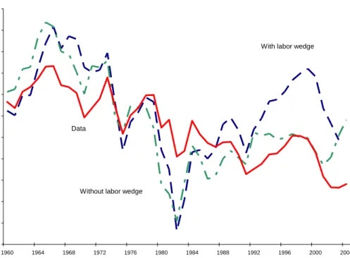
the rate of return for capital decreases in our model while it increases quickly in the data.14 Next we examine our model’s performance with respect to the U.S. saving rate. In Figure (7) we display the data and the model generated net national saving rates with and without the labor wedge between 1960 and 2004. Saving rates generated by the two models are remarkably similar to each other until late 1980s. They both capture the secular decline from 1960 up to early 1990s, as well as the annual ‡uctuations in the actual U.S. data. However, both models generate higher saving rates than those in the data for the 1960s and lower rates for 1980s.15 After early 1990s the model with the labor wedge predicts higher saving rates than the model without the wedge. The di¤erences in the saving rates between the two models grow in the 1990s. While the saving rate generated by the model without the labor wedge seems to mimic the data well for 1990s, we do not consider it a successful model since its performance along other dimensions as shown in Figure 1 is not satisfactory. Note that the major reason for our model’s unsatisfactory performance in the 1990s is not
1 4In the version of the model with the labor wedge the gap between the data and the model generated rate of return to capital in the 1990s disappears.
1 5Later in sensitivity analysis, we show that some of the large ‡uctuations obtained in these graphs are due to the perfect foresight assumption. When the TFP growth rate is assumed to be stochastic, the simulated saving rates display smaller ‡uctuations compared to the perfect foresight case. Households’ intertemporal behavior is subdued due to the lack of perfect foresight of the real return to capital. Other features of the saving rate do not change signi…cantly when the perfect foresight assumption is abandoned. This is consistent with the …ndings in McGrattan and Prescott (2007b).
0% 2% 4% 6% 8% 10% 12% 14% 16% 18% 20% 22% 1960 1964 1968 1972 1976 1980 1984 1988 1992 1996 2000 2004 Saving R ate
With labor wedge
Without labor wedge Data
Figure 7: Saving Rate with and without the Wedge
that the standard model misses any important frictions that distort the consumption-saving trade-o¤. Rather, as our previous analysis shows, it is because the standard model is unable to generate the hours boom and thus the after-tax rate of return to capital. On the other hand, the …nding that the saving rates generated by the two models are “similar” until the 1990s indicates that the model without the labor wedge is reasonably good in replicating the consumption-saving trade-o¤ in the actual economy for that period even though it misses the consumption-leisure trade-o¤. Consequently, we will rely on the standard model to further examine the factors behind the secular decline in the saving rate until 1990s.16
3.2.1 Basic Intuition
In order to understand the main factors behind the behavior of saving over this time period, we conduct several counterfactual experiments. We use the model without the labor wedge to carry out these counterfactual experiments.17 While we graph the results of the simulations
1 6We also examined the private and the government saving rates separately in the benchmark economy. Our results indicate that the simulated government saving rates look reasonably close to its counterpart in the data while the private saving rate captures all the discrepancies that were present in the earlier results for the net national saving rate.
1 7Notice that the model with the labor wedge is not truly suitable for running counterfactual experiments. For example, the wedge is calculated using the labor income taxes in the data. It would be impossible to run
and the data for the entire time period, our main focus is from 1960 to late 1980s where the standard theory seems to perform reasonably well.
The intuition on how our model ingredients might a¤ect the saving rate can be readily seen from a back-of-envelope calculation of saving rates in the steady state
S K
Y =
+n
( + )=(1 k) +
(2)
where =g11 denotes the growth rate of TFP factor. For simple analytical tractability, we
de…ne the saving rate here as the ratio of net saving to gross output. From equation (2), a decline in population growth rate, an increase in the depreciation rate, and a decline in the growth rate of TFP all cause a decline in the saving rate. By contract, a decline in capital income tax rate increases the steady-state saving rate. In particular, given our calibrated parameter values, a decline in the population growth rate from 1.8% in the 1960s to 1.0% afterwards and an increase in the depreciation rate from 4.3% before 1980 to 5% afterwards would together cause a decline in saving rate by 3 percentage points, ceteris paribus.18
3.2.2 Counterfactual Experiments
In our benchmark calibration, we used time series data for the TFP growth rate, population growth rate, depreciation rate, capital and labor income tax rates, and fraction of government expenditures in GNP. During 1960-2004 there was a signi…cant decline in the population growth rate and an increase in the depreciation rate. In addition, there was a decrease in the capital income tax rate and an increase in the labor income tax rate.19 To isolate the impact of these changes one at a time, we start with setting all exogenous variables equal to their averages over 1960-2004. Later we add the time series data for each exogenous variable one at a time.
Population and Depreciation: In our …rst counterfactual experiment we try to isolate the role of the declining population growth rate by simulating the saving rate in an economy where all the exogenous variables (TFP growth, G/Y, depreciation, tax rates, transfers to GNP) are set to their long-run averages except for the population growth rate. In Figure 8, the series labeled ‘Time series for population only’displays the saving rate that is generated by the model economy where the only time series data that is used in the simulations is the population growth rate. The quantitative impact of the population growth rate in this time period seems moderate, resulting in a 1-2% decline by early 1990s.
an experiment where labor income taxes are set to their steady state values while keeping the wedge at its given values.
1 8
We thank Ellen McGrattan for suggesting these calculations. 1 9Data are provided in the Appendix 7.6.
4% 6% 8% 10% 12% 14% 16% 18% 1960 1965 1970 1975 1980 1985 1990 1995 2000 Saving Rate
Time series for population only
Data
Time series for population and depreciation
Figure 8: Role of Population and Depreciation
Next we generate a saving rate where both the population growth rate and the depreci-ation rate are set to their time series values. The rest of the exogenous variables are kept at their long-run averages. The results of this experiment are displayed by the saving rate labeled ‘Time series for population and depreciation’. The increase in the depreciation rate and the decrease in the population growth rate together account for 3-4 percentage point decline in the saving rate by early 1990s. The di¤erence between the two simulated series also shows the impact of the deprecation rate alone in generating a decline in the saving rate especially in mid 1990s.
TFP Growth Rate: Next, we examine the model generated saving rate when the only time series data that is included in the simulations is the TFP growth rate.20 We set all the other exogenous variables equal to their long-run averages.
There are several interesting features of the model generated saving rate that is displayed in Figure 9. First, it shows signi…cant ‡uctuations that mimic the data rather well until 1975. Consistent with our intuition, a decline in the TFP growth rate between 1960s and 1980s causes a drop in the saving rate by about 2 percentage points. Between 1980s and 2004, however, the average TFP growth rate increases above its long-run trend. Accordingly, our
2 0Figure A2 in the appendix displays the TFP growth rate for the U.S. under several di¤erent measures of the capital stock.
0% 2% 4% 6% 8% 10% 12% 14% 16% 18% 20% 1960 1965 1970 1975 1980 1985 1990 1995 2000 Saving Rate Data
TFP Time Series Only
Figure 9: Role of TFP
model predicts an increasing saving rate from mid-1980s. Our …ndings indicate that the model generated saving rates would have been much higher in the late 1990s if they were only due to the movements in the TFP growth rate.
Overall, our results suggest that i) the decline in the population growth rate and the increase in the depreciation rate alone account for a 3-4 percentage point decline in the saving rate, ii) the decline in the TFP growth rate before 1980s contributes to about 2% of the decline in the saving rate during this period,iii) observed TFP growth rates alone would have caused the saving rate to be much higher in the 1990-1995 period, and, iv) the decline in the TFP growth rate in 2001 had a signi…cant negative impact on the saving rate.
4
Extension to A Two-Country Economy
In the previous section, we show that domestic factors alone play quantitative important roles in explaining the U.S. saving rate. In a closed economy, these factors, however, are also the driving forces for domestic investment. Therefore, the above setup is silent on the secular trend of current account balance. To explore the current account balance, we now open this economy up to introduce other factors that could potentially a¤ect the U.S. domestic investment.
4.1 The Environment
Consider a perfect foresight two-country growth economy. For each countryi=f1;2g;there is a stand-in household with Nti working-age members at datet. Households are assumed to own the capital,Kti;and rent it to businesses. The law of motion for the capital stock is given by equation 4:Both capital and labor are immobile across countries. We assume that there is a risk-free bond traded internationally each period. In this framework a representative household in country imaximizes
1 X t=0 tNi t(logcit+ log(1 hit)) subject to Bit+1+Cti+Xti+ Kti X i t Kti ' i 2 Bit 1 +rtB + 1 ih;t wtiHti+ritKti ik;t(rti it)Kti+T Rit it (3) Kti+1 = 1 it Kti+Xti (4) Bi0; K0i given,
where cit=Cti=Nti is per member consumption, hit=Hti=Nti is the fraction of hours worked per member of the household, is the subjective discount factor, is the share of leisure in the utility function, Htiis total hours worked by all working-age members of the household,
Bti is the beginning of period bond holdings by country i; rtB is international interest rate,
i
h;t and ik;t are tax rates on labor and capital income, respectively, at timet; witis the real
wage,T Ritis a government transfer, itis a lump sum tax,ritis the rental rate of capital, and
i
t is the time-tdepreciation rate in country i. The size of the household evolves over time
exogenously at the ratenit=Nti=Nti 1:Following the literature we have quadratic adjustment costs for each country’s capital accumulation represented by Ki
t Xi t Ki t 'i 2:21 In general,
adjustment costs lead to smoother ‡uctuations in the current account. This allows us to concentrate on understanding the secular patterns in the current account.22
The aggregate production function is given by
Yti =Ait Kti (Hti)1 ;
where is the income share of capital and At is total factor productivity, which grows
exogenously at the rate gti=Ait=Ait 1.
2 1
To make sure that the steady state in the economy with adjustment costs is the same as the one without, we set the parameter'iequal to the investment-capital ratio at the steady state, gi 11 ni 1 + i, where
the TFP growth rate gi;population growth rate ni and the depreciation rate i denote the values of their
counterparts on the balanced growth path. 2 2
In each country i, there is a government that taxes income from labor and capital (net of depreciation) and uses the proceeds to …nance exogenous streams of government purchases
Gitand government transfers T Rit:A lump sum tax itis used to ensure that the government budget constraint is satis…ed each period:
Git+T Rit= ih;twtiHti+ ik;t(rti it)Kti+ it:
In other words, it is the primary government de…cit in the model. National accounting identity is given by:.
Cti+Iti+Git+Bti+1 =Yti+Bti 1 +rtB :
or
Cti+Iti+Git+CAit=Yti+BtirtB=GN Pti
whereCAit=Bit+1 Btiis the current account balance for countryi; Iti =Xti+ Kti Xti Ki t
'i 2:
In Appendix 7.5, we provide the de…nition of competitive equilibrium for this two-country model and the equilibrium conditions.
4.2 Measurement and Calibration
Our analysis is limited by the number of countries for which we can get consistent estimates of several exogenous variables, in particular the TFP growth rate. Consequently, we restrict our analysis to the CA balance between the U.S. and the following group of OECD countries: Austria, Canada, Belgium, Denmark, Finland, France, Germany, Greece, Iceland, Ireland, Italy, Japan, Netherlands, Norway, Portugal, Spain, Sweden, Switzerland, and United King-dom. For simplicity we refer to these OECD countries as the Rest of the World (ROW). We derive TFP growth rates for the U.S. and the ROW using data from Groningen Total Economy Database. For the ROW, we generate aggregate output, capital, and hours as the weighted sum of each individual country’s output, capital and hours, all weighted by each individual country’s output share.23 Then we use the Solow decomposition to get aggregate TFP for the ROW. The TFP computed in this way di¤ers very little from the TFP computed as the weighted average of TFP of individual countries, weighted by each country’s output share. We also compute the average population growth rate of the ROW using the same weighting method.
2 3
The data on the capital stock is not available from Groningen Total Economy Database. To compute the real capital stock that is consistent with real GDP in constant 1990 dollars (converted at Geary Khamis PPPs), we collect the data of real total capital stock as a percentage of real GDP between 1960 and 2001 from the Kiel Institute database on capital stock in the OECD countries. We then multiply this ratio with real GDP from Groningen Total Economy Database to obtain data of real capital stock for each country. We impute the real capital stock after 2001 by multiplying the real total capital stock as a percentage of real GDP at 2001 and the real GDP in each of the last three years.
We measure the saving rate using savti= Y i t Git Cti itKti Yi t itKti ;
where Yti is GDP in countryi at time t: Similarly, we compute the current account de…cit as a percentage of GDP as
cait= B
i
t+1 Bti Yti :
Constant Parameters: There are four parameters that are time and country invariant throughout our analysis. The capital share parameter, ;is set to0:4. The capital adjustment cost parameter, , is set to 1, which is well within the range of values used in the literature.24 The subjective discount factor, ; is set to 0:9702so that the capital output ratio is 3:2 at the …nal steady state in the U.S. The share of leisure in the utility function, ;is set to1:45 to match an average workweek of 35 hours in the U.S.
Calibration of the Initial Conditions: We use the initial capital-output ratio for the U.S. in 1960, 3:5; to pin down the initial capital stock for the home country. We set the initial capital stock for the ROW to be 1.55 times that in the U.S.:which is the actual ratio of capital stocks between ROW and the U.S. in 1960. The initial foreign asset holdings,eb11960
andeb21960 are both set to be zero.
A crucial parameter for the results is the size of the U.S. relative to the ROW in 1960. This relative size determines the importance of the U.S. in shaping the world prices relative to the ROW. If the ROW is too small to impact the world prices then the model converges to the closed economy case with a zero current account balance for the U.S. In our benchmark calibration, we have chosen the relative size such that the current account de…cit generated by the model in 1960 is equal to its counterpart in the data.25 After the initial size is pinned down, the actual TFP and population growth rates determine the evolution of the relative size over time.26
Calibration of the 1960-2004 period: In our benchmark simulation, we use the actual time series data for the U.S. and the ROW between 1960-2004 for the TFP growth rate, gt 1; population growth rate, nt 1; share of government purchases in GDP, t;
and capital and labor income tax rates, k;t; h;t.27 The tax rate data for the U.S. and the
ROW comes from updated calculations of Mendoza, Tesar and Razin (1994) up to 1996. For
2 4
See, for example, Baxter and Crucini (1993, 1995), Fogli and Perri (2006). 2 5
As we change the initial relative size and make the ROW matter more and more in 1960, model generated current account surplus for the U.S. in 1960s and the current account de…cit in 2004 get implausibly large. In section 5.2 we present sensitivity analysis to this parameter.
2 6An alternative is to introduce an openness index as in McGrattan and Prescott (2007c) that would impact the role of the U.S. in shaping the world prices.
2 7
years after 1996 we set the tax rates equal to their 1996 values. For the ROW we set the depreciation rates t;and the shares of government transfers inGDP,T Rt=GDPt;equal to
the values in the U.S. All the data used in the paper are provided in the Appendix 7.6.
Calibration of 2005 and beyond: We assume that the U.S. and the ROW start from given conditions in 1960 and eventually converge to a steady-state in 2070. In our benchmark model, we set the seven exogenous variables in table 2 equal to their steady state values starting in 2005.28 Similar to our closed economy, we set the U.S. population growth rate after 2004 and at the steady state equal to 1%: Since projections for the ROW are not very di¤erent from the U.S. we set the steady state population growth in the ROW also equal to 1%.29 Also, we set the U.S. depreciation rate equal to5%for year 2005 and beyond, similar to our closed economy. For the OECD countries we use the same depreciation rates as the U.S. Again, our results are not sensitive to di¤erent assumptions about the calibration of most of the variables for the period 2005 and beyond.
Table 2: Parameter Values for 2005 and Beyond, Open Economy
U.S. ROW
gt 1 TFP Growth Rate 0.011 0.011 nt 1 Population Growth Rate 0.01 0.01
t Government Purchases to GDP Ratio 0.16 0.18
t Depreciation Rate 0.05 0.05
T Rt=GDP Transfers to GDP Ratio 0.08 0.08 k;t Capital Income Tax Rate 0.42 0.34 h;t Labor Income Tax Rate 0.29 0.38
4.3 Numerical Solution
Detrending: For an aggregate variable of each country i, denoted as zti; its detrended version is given by: zeti=Zti=h Ait
1
1 Ni
t
i
:Note that for each country, an aggregate variable is detrended by its own TFP factors and population size. The detrended international bond
consumption expenditures in national currency units for each country from OECD annual national accounts. Data on transfer for the U.S. is obtained from National Income and Product Acocunts. We use the same data for the OECD countries. We obtain data on population from 15-64 years old from UN demographic year book (1960-1969) and OECD Economic Outlook (1970-2005).
2 8
With our assumed tax rates, the government budget in the U.S. will be in a surplus at the steady state. 2 9
Population growth rates are the growth rates of civilian non-institutional population 16 years and over reported by the BLS. Population projections are taken from U.S. Bureau of the Census (http://www.mnforsustain.org/united_states_population_growth_graph.htm)
market clearing equation is
eb1t+1= eb2t+1st+1 (5)
where we follow McGrattan and Prescott (2007c) and denote st+1 = A2 t+1 A1 t+1 1 1 N2 t+1 N1 t+1 as the
relative size of the two countries. Note that we can solve recursively for the entire sequence of st+1 fromst+1=st g2 t+1 g1 t+1 1 1 n2 t+1 n1
t+1 ;given s0 and the sequence of g i
t; nit t=0;1;::1:
Algorithm to compute the transition path and the steady-state: Given the steady state net foreign asset distribution
n eb1;eb2
o
, we can solve for other macro variables in the steady state. However, the steady state net foreign asset distribution depends critically on the transition path and the initial asset distribution.30 Therefore we need to solve for
the transition path and the steady state simultaneously. Note that for equations (20) and (21) to hold for each country at the steady state, it must be g1 = g2 at the steady state. Similarly, for the relative size of the country to be stationary, we haven1 =n2:
We assume that the economy reaches steady state at some future date T: Then start-ing from some initial asset distribution nek1
0;ek20;eb10;eb20
o
; we can solve for the entire path of nec1t;ec2t; rBt ;ek1t+1;ekt2+1;eb1t+1;eb2t+1; h1t; h2to Tt=0 using the system of nonlinear equations (13), (20);(21);(23) and(5):To rule out Ponzi schemes, we require that at the steady state
ebiT+1 giT 1 1 ni T 1 +rBT = (1 iT) ekTi hiT 1 e ciT xeit
so that agents will not borrow in…nitely. Note however, it is possible that at the steady state
ebi 6= 0:
4.4 Results for the Open Economy
We start this section by showing the saving and investment rates obtained for the U.S. economy in the open economy setting without the labor wedge. A notable di¤erence between the saving rate generated in this case as shown in Figure 10 and the earlier closed economy case in …gure 7 is the lack of the sharp decline in the saving rate in 1980s that was present in the earlier case. This is due to the assumption of adjustment costs present in the open economy version.
We now present the model generated current account balances and the data. Figure 11 shows that our model generated CA balance captures quite well the overall secular decline in the observed CA balance since 1960s. In particular, both series start from a surplus of around 0.3% in 1960 and end up with a CA de…cit about 2% in 2004. This result indicates that it is possible to generate realistic current account de…cits for the U.S. in a carefully calibrated standard neoclassical growth model.
3 0As Chattejee (1994) shows in a complete market economy there are in…nite number of steady state wealth distributions.
1960 1970 1980 1990 2000 0.04 0.06 0.08 0.1 0.12 0.14 0.16 0.18 0.2 0.22 year Sa vin g R a te model data 1960 1970 1980 1990 2000 0.04 0.06 0.08 0.1 0.12 0.14 0.16 0.18 0.2 0.22 year In ve stme n t R a te model data
-2.5% -2.0% -1.5% -1.0% -0.5% 0.0% 0.5% 1.0% 1.5% 1960 1964 1968 1972 1976 1980 1984 1988 1992 1996 2000 2004 Data Model
Figure 11: Currrent Account Balance as a Percentage of GDP, Benchmark
4.4.1 Counterfactual Experiments
As in the closed economy case, we conduct several counterfactual experiments to understand the driving forces behind the CA de…cits found in our framework. Figure 12 shows that the secular trends in the TFP growth rates between the U.S. and the ROW have been quite di¤erent. Notice that ROW display higher TFP growth in the 1960s relative to the U.S. The country that is mostly responsible for that measurement is Japan. In our framework where there is free trade, the model implies that capital should ‡ow from the U.S. to the ROW in the 1960s. We also observe the trend TFP growth rates to reverse in the late 1990s where U.S. TFP growth exceeds that of the ROW indicating capital should ‡ow to the U.S. This motivates us to investigate the role of the TFP growth rate versus the other exogenous variables which include the population growth rate, tax rates, and the share of government expenditures in GNP.
In our …rst counterfactual experiment we examine what would have happened to the CA balance of the U.S. if the ROW had the same TFP growth rates as the U.S. throughout this period.31 The only di¤erences between the U.S. and the ROW in this case are due to the di¤erences in the population growth rates, G/Y, and tax rates. The result of this
3 1Similar to the closed economy case, we use the economy without the wedge to run the counterfactual experiments.
0.96 0.97 0.98 0.99 1 1.01 1.02 1.03 1.04 1.05 1.06 1960 1964 1968 1972 1976 1980 1984 1988 1992 1996 2000 2004 U.S. ROW
Figure 12: TFP Growth Rates
experiment is depicted in …gure 13. The line ‘Identical TFP growth’shows the CA balance that would have resulted in the U.S. economy if the ROW had the same TFP growth rates as the U.S. In this experiment the model implied current account surpluses of the 1960s disappear. In addition, the CA de…cit in 2004 declines from 2.2 % in the benchmark case to 1%. More importantly, the current account balance implied in this case does not display a trend. Similar results are obtained when population growth rate, G/Y, and tax rates are introduced one at a time.32 Our …ndings cast doubt on the quantitative importance of the di¤erential aging of populations in explaining the secular decline in the U.S. current account balance.
In the second counterfactual experiment, we shut down all the exogenous di¤erences between the ROW and the U.S. except for the di¤erences in TFP growth rates. We use the population growth rate, G/Y, and the tax rates that prevail in the U.S. for both the U.S. and the ROW. The only country speci…c exogenous variable we allow for is the TFP growth rate. Figure 14 displays the resulting CA balance labeled as “ROW same as U.S. except for TFP growth”. The secular decline in the U.S. CA balance clearly comes from the di¤erences
3 2
The relatively constant 1% CA de…cit obtained in this counterfactual experiment comes mostly from the higher labor taxes in the U.S. and the di¤erences in the level of capital stock that existed between the U.S. and the ROW in 1960. If we force the U.S. and the ROW to have the same initial levels of capital we get a ‡at current account de…cit of 0.5%.
-2.5% -2.0% -1.5% -1.0% -0.5% 0.0% 0.5% 1.0% 1.5% 1960 1964 1968 1972 1976 1980 1984 1988 1992 1996 2000 2004 Benchmark Identical TFP growth Data
Figure 13: CA Balance as a Percentage of GDP, Identical TFP Growth
in TFP growth rates in this exercise. These di¤erences drive up the U.S. investment demand relative to savings resulting in an increase in the U.S. current account de…cit. These results are robust to alternative measures of TFP which are shown in …gure A2 in the Appendix 7.2.
In summary, our …ndings suggest that the secular decline in the U.S. CA balance may be due to the di¤erences in the TFP growth rates between the U.S. and the ROW. In other words, the standard growth model may be able to capture the secular movements in the current account against OECD countries reasonably well once di¤erences in key exogenous variables, in particular the TFP growth rate across countries is incorporated into the analysis.
5
Sensitivity Analysis
In this section we will examine the sensitivity of our results to some of the modelling as-sumptions and parameter choices
5.1 Closed Economy
-2.5% -2.0% -1.5% -1.0% -0.5% 0.0% 0.5% 1.0% 1.5% 1960 1965 1970 1975 1980 1985 1990 1995 2000 2005 Data Benchmark
ROW same as U.S. except for TFP Growth
Figure 14: CA Balance as a Percentage of GDP, Only TFP Growth Di¤erent
5.1.1 Alternative Assumption on Values for 2005 and Beyond
Our procedure for assigning values to TFP growth rates between 2005 and the …nal steady-state is arbitrary. In our benchmark calculations we set the TFP growth rate equal to its 1960-2004 average right after 2004. To check the sensitivity of our results to this assumption, we report simulations from a case where we assume the TFP growth rate to continue at its 2004 level which is higher than its steady state value. In Figure 15, the vertical line represents the year 2004 beyond which the two simulated saving rates di¤er only because of the assumed values for the TFP growth rate for 2005 and beyond. There are noticeable di¤erence in the 1990-2004 period between the two series. However, the two series are virtually identical until the 1990s which is one of the reasons why focus our results up to the 1990s.33
5.1.2 No Perfect Foresight
So far we have assumed perfect foresight. Households know the entire time path of all exogenous variables. In this section, we will summarize our …ndings from two alternative
3 3
Among the exogenous variables for which we had to make assumptions about future values, TFP growth rate was the most imporant. Di¤erent assumptions about the values of the rest of the exogenous variables for 2005 and beyond had insigni…cant consequences in the results up to 2004.
0% 5% 10% 15% 20% 25% 1960 1970 1980 1990 2000 2010 Saving Rate High future TFP Low future TFP Data
Figure 15: Role of the Future
assumptions on expectations for the TFP growth rate while we still feed in the time path of all the other exogenous variables deterministically.
Adaptive Expectations: Our …rst alternative expectations scheme is a simple adaptive framework where expectations of future TFP growth rates are formed according to
get+1 =gte+ (gt gte):
Here, the parameter 2 [0;1] re‡ects the extent to which expectations will change as a result of past errors. A near zero indicates near-static expectations whereas a near unity suggests setting expectations equal to the most recently observed actual growth rate. In the latter case, the model’s saving rate would essentially shift one period hence relative to our perfect foresight case.
Figure 16 displays observed saving rates and a collection of simulated saving rates indexed by a few values of : Even the near-static expectations cases with low values of generate saving rates with similar features compared to the deterministic case. The secular movements are reasonably well-represented, but the model does a poor job in the 1980s and early 2000s.
Stochastic TFP Growth Rate: Another alternative formulation is to assume that TFP growth rate follows an AR(1) process.34 Estimating this simple process yields a
per-3 4We solve the decision rules in this model by using the …nite element method following McGrattan (1996). We assume that agents have perfect foresight for all other exogenous variables by specifying a degenerate transition matrix with forty-six states. In this matrix, each state refers to a vector of exogenous series
0% 2% 4% 6% 8% 10% 12% 14% 16% 18% 20% 1960 1965 1970 1975 1980 1985 1990 1995 2000 Saving Rate λ=0.2 λ=0.4 Data
Figure 16: Saving Rate with Adaptive Expectations
sistence coe¢ cient of 0.33 (with an intercept term 0.69 and a standard error of regression 0.0224).
Figure 17 depicts the actual saving rate and the model generated saving rate when households forecast future TFP growth rates using the estimatedAR(1)process given above. The simulated saving rate is fairly close to the actual saving rate. The AR1 assumption for the TFP growth rate produces smoother saving rates compared to the perfect foresight case. Households’intertemporal behavior is subdued due to the lack of perfect foresight of the real return to capital.
5.2 Open Economy
There are two parameters that play an important role in the results regarding the model generated current account balances. These are the adjustment cost parameter,aaa, and the size of the ROW, N2. Both of these parameters have an impact on the size of the capital ‡ows. For example, as the size of the ROW gets smaller the model gets closer to a closed
corresponding to a particular year and the transition probabilities from year j to j+ 1 (j 2004) is one. We set the vector of exogenous series corresponding to year 2005 as the steady state vector speci…ed in the calibration section. Also, we set the last diagonal of this matrix to one which indicates that after 2005 the exogenous variables will stay at their 2005 values.
0% 2% 4% 6% 8% 10% 12% 14% 16% 18% 1960 1965 1970 1975 1980 1985 1990 1995 2000 2005 Savin g Ra te Data AR(1) TFP growth
Figure 17: Saving Rate with AR(1)
economy model. As this parameter gets larger, the size of the capital ‡ows increase. Figure 18 displays the current account balances generated by the model for di¤erent N2’s. As the size of the ROW gets larger, the current account surpluses in the 1960s and the current account de…cits in the later periods get larger.
Figure 19 displays the current account balances for di¤erent values of the adjustment cost parameter. As the adjustment costs decline the current account surpluses of the 1960s and the de…cits in the later periods gets larger.
The sensitivity analysis in this section reveals that the model economy generates current account de…cits in the later periods under a large set of parameters.
6
Concluding Remarks
The U.S. national saving rate and the current account balance have experienced a secular decline since the 1960s. A popular answer for the decline in the national saving rate has been the decline in the private saving of the baby boom generation in response to an increase in the generosity of the social security program. In this paper, we abstract from life cycle features and social security, and employ a standard growth model calibrated to the U.S. economy. Our in…nite horizon, complete markets setup captures the decline in the U.S. saving rate reasonably well. The important factors responsible for the secular decline between 1960 and
-0.15 -0.1 -0.05 0 0.05 0.1 1960 1965 1970 1975 1980 1985 1990 1995 2000 2005 CA balance Dat Benchmark, N2=0.2 N2=0.6 N2=1.0 N2=2.0 Figure 18: Sensitivity to N2 -0.2 -0.15 -0.1 -0.05 0 0.05 0.1 0.15 1960 1965 1970 1975 1980 1985 1990 1995 2000 2005 CA balance aaa=0.6, benchmark aaa=0.4 aaa=0.35 Data
early 1990s are i) the decrease in the population growth rate, and ii) the increase in the depreciation rate. The time path of observed TFP growth rates does not exhibit a trend but help explain the year-to-year ‡uctuations in the saving rate over this time period. When we examine the role of these factors on the U.S. current account, we discover that di¤erences in TFP growth rates between the U.S. and its trading partners play a signi…cant role.
The remaining puzzle is the hours boom and the continuous decline in the saving rate since 1990s. Theories put forward would have to feature signi…cant changes in an element missing from the standard model since the 1990s. It is possible that intangible capital as discussed by Corrado, Hulten, and Sichel (2006) and McGrattan and Prescott (2007a) might be the missing link. Direct calculations of intangible capital will be needed to modify the de…nition of savings in order to examine if it can be successful in mimicking the hours boom (as shown in McGrattan and Prescott (2007b)) and the change in savings since 1990s at the same time. These issues together with a more detailed study of the 1990s, and the implications of a life-cycle model as in Chen, ·Imrohoro¼glu and ·Imrohoro¼glu (2007) are left for future research.
7
Appendix
7.1 Competitive Equilibrium of the Closed Economy
De…nition of Competitive Equilibrium:Given a government policyfGt; T Rt; h;t; k;t; tg1t=0,
a competitive equilibrium consists of an allocationfCt; Xt; Ht; Kt+1; Ytg1t=0and price system fwt; rtgsuch that
given policy and prices, the allocation solves the household’s problem,
given policy and prices, the allocation solves the …rm’s pro…t maximization problem with factor prices given by: wt= (1 )AtKt(Ht) ;and rt= AtKt 1(Ht)1 ;
the government budget is satis…ed,
and the goods market clears: Ct+Xt+Gt=Yt:
Equilibrium Conditions: The equilibrium conditions of this model can be described in three equations below:
ht 1 ht = (1 h;t)(1 ) Yt Ct ; (6) Ct+1 Nt+1 = Ct Nt n 1 + (1 k;t+1) h At+1Kt+11(Ht+1)1 t+1 io ; (7) Kt+1 = (1 t)Kt+AtKt(Ht)1 Ct Gt: (8)
Detrending: For an aggregate variable zt; its detrended version is given by: ezt = zt= A
1 1
t Nt :Applying this change of variables to (7) and (8), we obtain equations
e ct+1 = e ct g 1 1 t+1 n 1 + (1 k;t+1) h xt+11 t+1 io ; e kt+1 = 1 g 1 1 t+1nt+1 [(1 t) + (1 t)xt 1]ekt ect;
where t is the ratio of government purchases to output,Gt=Yt;andxt is detrended
capital-labor ratio,(Kt=Ht)=A 1 1
t :
Steady-state: Setting zet = ze for all t; we obtain the following steady-state for the
model: e h 1 eh = (1 eh)(1 ) e y ec 1 = 1 g11 n 1 + (1 ek) h x 1 eio e k = 1 g11 n [(1 e) + (1 e)x 1]ek ec:
These equations are solved for the steady-state values of detrended capital, consumption and hours worked where e; eh; and ek are the steady-state depreciation, labor income tax
rate and capital income tax rate, respectively. The steady-state saving rate is given by
e s= (g 1 1 n 1)ek e y eek : (9)
7.2 Details of the Calibration of the Closed Economy
In this section, we provide the details of our calibration for the closed economy. We use data from the 2005 revision of National Income and Product Accounts (NIPA) and Fixed Asset Tables (FAT) of Bureau of Economic Analysis (BEA) for the years 1960-2004.
Denote measured GNP as follows
(cs+cnd+icd) +g+i+nx+nf p=GN P =dep+N N P; (A-1) where cs; cnd; icd denote real personal consumption expenditures on services, nondurables and durables, g denotes the sum of government consumption, denoted asgc;and gross gov-ernment investment, denoted as gi; idenotes gross private domestic investment, nxdenotes net export, nf p denotes net factor payments to the rest of the world, and dep denotes consumption of …xed capital.
Our adjustments to measured macroeconomic aggregates follow Cooley and Prescott (1995). First, we add government capital to measured capital stock. When we add the service ‡ow from the government capital stock,sg;to measured GNP, A-1 becomes
(cs+cnd+icd+sg) +gc+ (i+gi) +nx+nf p=GN P+sg =dep+ (N N P +sg); (A-2) where dgi denotes depreciation of government …xed assets and dep dgiis depreciation of private …xed assets.
Second, we add the stock of consumer durables to measured capital stock. Including the service ‡ow from the stock of consumer durables, csd;to measured GNP changes A-2 to
(cs+cnd+csd+sg) +gc+ (i+nicd+dcd+gi) (A-3) +nx+nf p = GN P +sg+csd
= (dep+dcd) + (N N P +sg+csd dcd);
where dcd denotes the depreciation of the stock of consumer durables. Therefore, total private consumption becomes (cs+cnd+csd+sg) and total domestic investment becomes (i+icd+gi)or(i+nicd+dcd+gi), wherenicdis referred to as net investment in the stock of consumer durables and dcd denotes the depreciation of the stock of consumer durables. Total depreciation becomes(dep+dcd):
Third, we add net foreign assets to measured capital stock. The service ‡ow from this stock is already measured as nf pin GNP. We reorganize A-3 as
(cs+cnd+csd+sg) +gc (10)
+(i+nicd+dcd+gi+nx+nf p) = GN P +sg+csd (11) = (dep+dcd) + (N N P +csd+sg dcd);
where total domestic investment is now de…ned as (i+nicd+dcd+gi+nx+nf p):
Following McGrattan and Prescott (2000), we assume that the rate of returns for the stock of consumer durables and government …xed assets are equal to the rate of return for non-corporate capital stock. Speci…cally, we have
i = (Accounting Returns + Imputed Returns)
(Non-corporate capital+Land+Inventory Stock+Capital of Foreign Subsidiaries) = (0:0603 + 1:6803i)
(2:976 + 0:0095=i);
where 0.0603 is non-corporate pro…t plus net interest less intermediate …nancial services, 1.6803 is the sum of the net stock of government capital, the stock of consumer durables, land and inventory stock, 2.976 is the sum of net stock of non-corporate business, government capital, stock of consumer durables, land and inventory stock, and 0.0095 is the net pro…t from foreign subsidiaries.
The above equation gives a value of 3.93% foriover the period between 1960 and 2000. The service ‡ows the stock of consumer durables and government capital, Ysd and Ysg;
respectively, are computed following Cooley and Prescott (1995):
Ysd = csd= (i+ d)KD; Ysg = (i+ g)KG:
Then the capital share of output, ;is given by
= Ykp+Ysd+Ysg
GN P +Ysd+Ysg ;
where Ykp is the income ‡ow from private …xed assets,
Ykp = Unambiguous Capital Income+ p (Proprietors’Income (A-5)
+Indirect Business Taxes)+Depreciation (12)
= p GN P:
This gives a value of0:32 for p and a value of0:41 for :
De…ne the net national saving rate as
s = Y CON GOV DEP R
Y DEP R
= (GN P +sg+csd) (cs+cnd+csd+sg) gc (dep+dcd) (GN P +sg+csd) (dep+dcd)
= GN P cs cnd gc (dep+dcd)
N N P +csd+sg dcd :
Since in our model the government does not issue debt or lend to households, we de…ne the primary government saving rate as
sgov= Tax Revenue (gc+tr) Net Interest Payment on Government Debt
Y DEP R ;
where tr is net government transfers, computed as current transfer payments minus current transfer receipts. Accordingly, the private saving rate is computed as
psav=s sgov:
In Figure A1 we compare the data on the net national saving rate (net national saving as a percent of NNP) from the NIPA with the net national saving rate that results after all the adjustments discussed above are made to the data.
0% 2% 4% 6% 8% 10% 12% 14% 16% 18% 1960 1965 1970 1975 1980 1985 1990 1995 2000
Net National Saving - NIPA
Net National Saving -Adjusted
Figure A1: NIPA and the Adjusted Saving Rate
In our benchmark economy we have de…ned capital to include the stock of consumer durables, government capital, and foreign capital. These adjustments to capital came with corresponding adjustments on the measurement of GNP as explained above. In Figure A2 we display four di¤erent TFP growth rate measures. One of these measures is the TFP growth rate used by Jorgenson (2003). The other three are growth rates obtained under di¤erent assumptions on the capital stock. In particular, we display TFP growth rates under the i) benchmark de…nition of the capital stock, ii) benchmark de…nition minus land, and, iii) benchmark de…nition minus the stock of consumer durables and government capital. This exercise demonstrates that measured TFP growth rates are not very sensitive to the de…nition of the capital stock.