Robust fitting of mixture of factor analyzers using the trimmed likelihood estimator

ROBUST FITTING OF MIXTURE OF FACTOR ANALYZERS

USING THE TRIMMED LIKELIHOOD ESTIMATOR

by

LI YANG

B.S., Southwest University, China, 2011

A REPORT

submitted in partial fulfillment of the

requirements for the degree

MASTER OF SCIENCE

Department of Statistics

College of Arts and Sciences

KANSAS STATE UNIVERSITY

Manhattan, Kansas

2014

Approved by:

Major Professor WEIXIN YAO

Copyright

LI YANG

Abstract

Mixtures of factor analyzers have been popularly used to cluster the high dimensional data. However, the traditional estimation method is based on the normality assumptions of random terms and thus is sensitive to outliers. In this article, we introduce a robust estimation procedure of mixtures of factor analyzers using the trimmed likelihood estimator (TLE). We use a simulation study and a real data application to demonstrate the robustness of the trimmed estimation procedure and compare it with the traditional normality based maximum likelihood estimate.

Key words: EM algorithm, Factor analysis, Mixture models, Robustness, Trimmed likeli-hood estimator.

Table of Contents

2 Mixtures of Factor Analyzers 3

2.1 Single factor analysis . . . 3

2.2 Mixtures of factor analyzers . . . 4

3 Robust Fitting of Mixtures of Factor Analyzers Using the Trimmed

Like-lihood Estimator (TLE) 7

4 Simulation Study and Real Data Application 10

4.1 Simulation study . . . 10

4.2 Real data application . . . 12

5 Discussion 19

Bibliography 23

List of Figures

4.1 Wine data: Plot of the estimated posterior means of theq= 2 factors (4,◦, and ∗ denote true component membership). . . 14

List of Tables

4.1 Average (Std) of MCP, with n= 200. . . 12

4.2 Average (Std) of MCP, with n= 400. . . 13

4.3 Average (Std) of Euclidean distance, with n= 200. . . 15

4.4 Average (Std) of Euclidean distance, with n= 400. . . 16

4.5 Wine data: Estimated Means withα = 0,0.01, and 0.03. . . 17

Acknowledgments

First and foremost, I would like to express my appreciation to my major professor, Dr. Weixin Yao, for all his encouragement, guidance and suggestions.

I would also like to thank Dr. Weixing Song and Dr. Christopher Vahl for their willing-ness to serve on my committee and for their valuable insight.

My gratefulness extends to everyone who supported me in any respect during the com-pletion of the report.

Chapter 1

Introduction

Factor analysis is a statistical dimension reduction technique for modeling the covariance structure of high dimensional data using a small number of latent variables (Ghahramani and Hinton (1997)). It can be extended by allowing different local factor models in different regions of the input space. This results in a model which performs clustering and dimension reduction at the same time, and can be thought as a reduced dimension mixture of Gaussians. Ghahramani and Hinton (1997) and Hinton et al. (1997) originally proposed mixtures of factor analyzers (MFA) model. They used this model to visualize high dimensional data in a lower dimensional space to explore the group structure. Tipping and Bishop (1997, 1999) and Bishop (1998) considered the related model of mixtures of principal component analyzers for the same purpose. MFA model is in fact a nonlinear model which can be considered as a combination of traditional factor analysis (FA) model and the analysis of finite mixture models. Therefore, MFA model offers a way to overcome the linear limitation of the traditional FA model. In recent years, MFA model has received considerable interest. See, for example, Fokou´e and Titterington (2003), Yung (1997), Dolan and VanderMaas (1998), and Arminger et al. (1999). McLachlan et al. (2003) discussed the application of mixtures of factor analyzers to density estimation and the clustering of high-dimensional data.

MFA has been traditionally fitted using the maximum likelihood estimator (MLE) based on the normality assumptions of random terms. Ghahramani and Hinton (1997) introduced

an exact Expectation-Maximization (EM) algorithm to compute the MLE of MFA. However, it is well known that the normal based MLE can be very sensitive to outliers. In fact, even a single outlier can make an enormous impact on the MLE, which in mixture models means that at least one of the component parameters estimation might be affected extremely large. In this report, a robust fitting of mixtures of factor analyzers is introduced based on the idea of trimmed likelihood estimator (TLE) (Neykov et al., 2007). The TLE is designed to fit the majority of the data, whereas the remaining data will be considered as outliers and thus will not be used for parameter estimation. We use a simulation study and a real data application to demonstrate the robustness of the new estimation procedure and compare it with the traditional normality based maximum likelihood estimate.

The rest of the report is organized as follows. In Chapter 2, we briefly introduce the EM algorithm for a single factor analysis (FA) and the mixture of factor analyzers (MFA). Chapter 3 presents the robust fitting of the mixture of factor analyzers using the trimmed likelihood estimator (TLE). Simulation results and real data application are presented in Chapter 4. A discussion section ends the report.

Chapter 2

Mixtures of Factor Analyzers

2.1

Single factor analysis

Let y₁, ...,y_n be a random sample of size n on a p-dimensional random vector. A typical single factor analysis model is given by:

y_i =µ+ Λzi+ei, i= 1, ..., n, (2.1)

where µ is the mean of y, zi is a q-dimensional (q < p) vector of latent or unobservable

variables called factors, and Λ (p×q) is a factor loading matrix. The factorsziare assumed to

be i.i.d. Nq(0

¯,Iq), independent of the errorsei, which are assumed to be i.i.d. Np(0¯,Ψ) with Ψ a diagonal matrix Ψ = diag(σ2

1, ..., σ2p).The marginal density ofyis thenNp(µ,ΛΛT+ Ψ).

For the purpose of classifying and reducing data, the traditional single factor analysis is a useful tool for reducing a mass of information to an efficient description and grouping interdependent variables into descriptive categories. In statistics, it is a method used for explaining data, in particular, correlations between variables in multivariate observations.

The single factor analysis model (2.1) can be fitted by maximizing the log-likelihood:

`(θ) = n X i=1 log{(2π)p/2|ΛΛT _{+ Ψ|}−1/2_exp[−1 2(yi−µ) T_(ΛΛT _{+ Ψ)}−1_(y i−µ)]},

with θ = (µT,ΛT,ΨT)T, which can be computed iteratively via the EM algorithm if zi is

E-step: Given the current estimator θ(k), calculate the following conditional expectation given the observed data y:

a(_ik)=E(zi|yi,θ (k)_{) = Λ}(k)T_(Ψ(k)_{+ Λ}(k)_Λ(k)T₎−1_y i, b(_ik) =E(zizTi |yi,θ (k)_{) =I −Λ}(k)T_(Ψ(k)_{+ Λ}(k)_Λ(k)T₎−1_Λ(k) +{Λ(k)T(Ψ(k)+ Λ(k)Λ(k)T)−1y_i}{Λ(k)T(Ψ(k)+ Λ(k)Λ(k)T)−1y_i}T. M-step: Calculate µ(k+1) = n X i=1 (y_i−Λ(k)a(_ik)), Λ(k+1) =n n X i=1 y_i(a(_ik))Ton n X i=1 b(_ik)o −1 , Ψ(k+1) = 1 ndiag n X i=1 (y_iyT_i −Λ(k+1)a(_ik)yT_i ) .

2.2

Mixtures of factor analyzers

Although the single factor analysis model (2.1) provides a global linear model for the presen-tation of the data in a lower-dimensional subspace, its application is limited when the data is not homogenous. The mixtures of factor analyzers model (MFA), which allows different local factor models in different regions of the input space, is a natural extension of the single factor analysis. Assume we have a mixture of m factor analyzers with mixing proportion

πj,j = 1, ..., m. The marginal density ofy is given by:

f(y;θ) = m X j=1 πjNp(y;µj,ΛjΛTj + Ψ), (2.2) where θ = (πT_,µT_,ΛT_,ΨT₎T_{, π = (π} 1, ..., πm−1)T, µ = (µT1, ...,µTm)T, Λ = (ΛT1, ...,ΛTm)T.

Here, µ_j is the mean of the jth _{component, Λ}

j is the factor loading matrix of the jth

the estimation equations to have a definition of the mixture factor analyzers in terms of conditional densities. For the jth _{component, the conditional density function is:}

fj(y|z) =Np(y;µj+ Λjz,Ψ).

Within each component of the mixture, we have the following joint density of yand z: y z ∼ Np+q µ_j 0 , ΛjΛTj + Ψ Λj ΛT_j Iq .

Similar to the single factor analysis, the mixture of factor analyzers can be estimated by maximizing the following likelihood:

`(θ) = n X i=1 log m X j=1 πj h (2π)p/2|ΛjΛTj + Ψ| −1/2_exp{−1 2(yi−µj) T_(Λ jΛTj + Ψ) −1_(y i−µj)} i , (2.3) However, there is no explicit solution for the above maximizer. Ghahramani and Hinton (1997) introduced an EM algorithm to maximize (2.3). More specifically, let ωij be an

indicator variable indicating from which component does y_i come. That is,

ωij =

1, if y_i is from jth _component,

0, otherwise. (2.4)

Then the complete log-likelihood for {(y_i,zi, ωij), i= 1, . . . , n, j = 1, . . . , m} is

`c(θ) = n X i=1 log m Y j=1 h πj(2π)p/2|Ψ|−1/2exp{− 1 2(yi−µj −Λjzi) T_Ψ−1_(y i −µj −Λjzi)} iωij .

The EM algorithm iterates between E-step, which computes the expected complete log-likelihood given current parameter estimates, and M-step, which maximizes the expected completed log-likelihood calculated in the E-step. We summarize the EM algorithm to maximize (2.3) as follows:

E-step: Given the current estimator θ(k), calculate the following conditional expectation given the observed data y:

E(ωij|yi,θ (k) ) = π (k) j Np(yi;µ (k) j ,Λ (k) j Λ (k) j T + Ψ(k)₎ Pm j=1π (k) j Np(yi;µ (k) j ,Λ (k) j Λ (k) j T + Ψ(k)₎ =p(_ijk),

a(_ijk)=E(zi|yi, ωij = 1,θ(k)) = Γ (k) j (yi−µ (k) j ), b(_ijk) =E(zizTi |yi, ωij = 1,θ(k)) = I−Γ (k) j Λ (k) j + Γ (k) j (yi−µ (k) j )[Γ (k) j (yi−µ (k) j )] T_, where Γj = ΛTj(Ψ + ΛjΛTj) −1_. M-step: Calculate π_j(k+1) = 1 n n X i=1 p(_ijk), µ(_jk+1) = ( _n X i=1 p_ij(k)(y_i−Λ_j(k)a(_ijk)) ) ( _n X i=1 p(_ijk) )−1 , Λ(_jk+1) = ( _n X i=1 p_ij(k)(y_i−µ_j(k+1))(a(_ijk))T ) ( _n X i=1 p(_ijk)b(_ijk) )−1 , Ψ(k+1) = 1 ndiag ( _n X i=1 m X j=1 p(_ijk) y_i−µ_j(k+1)−Λ(_jk+1)a(_ijk) y_i−µ(_jk+1)T ) .

Chapter 3

Robust Fitting of Mixtures of Factor

Analyzers Using the Trimmed

Likelihood Estimator (TLE)

The maximum likelihood estimator introduced in Chapter2is easy to implement, but is very sensitive to outliers. Even a single outlier can make an enormous impact on the MLE, and make at least one of the component parameters to be arbitrarily large. To overcome this, McLachlan et al. (2007), Andrews et al. (2011), and Baek and McLachlan (2011) proposed mixtures of t−factor analyzers by assuming multivariate t−distributions for component errors and factor distributions. In this chapter, we apply the idea of trimmed likelihood estimator (TLE) proposed by Neykov et al. (2007) be consistent to fit the the mixtures of factor analyzers in a robust way.

Suppose a number k (k ≤n) of n observations are regular observations in the data, and the remainingn−kobservations may be gross or outliers. The basic idea of TLE is removing the n−k observations which do not follow the model, and use only the k observations to fit the model. The combinatorial nature of the TLE can be expressed as:

max I∈Ik max θ X i∈I logf(y_i;θ),

whereIk is the set of allk-subsets of (1, . . . , n) and f(y;θ) is defined in (2.2). The fact that

all possible n_k partitions of the data have to be fitted by the MLE makes the estimation procedure very computational expensive. To find an approximative TLE solution for large

data sets, an algorithm called FAST-TLE was developed by Neykov and M¨uller (2003). The basic idea behind FAST-TLE algorithm contains two steps: a trial step followed by a refinement step.

(i) Trial step: Randomly select a subsample of size k∗ from the data sample and then fit the model to that subsample to get a trial maximum likelihood estimate (MLE).

(ii) Refinement step: This step is based on the so-called concentration procedure.

(a) Starting with the trial MLE, find a combination with the k smallest negative log-likelihoods based on the current estimate.

(b) Obtain an improved estimator by fitting the model to thesek cases. (c) Repeat (a) and (b) until convergence.

At the end of this step, the solution with the greatest trimmed likelihood value is stored. This value may not be guaranteed to be the global greatest but it would be a close approximation to it.

The choice of trail size k∗ and refinement subsample sizek are related to breakdown point (BP). The breakdown point (i.e., the smallest fraction of contamination that can cause the estimator to take arbitrary large values) of TLE was studied by using d-fullness technique. Vandev and Neykov (1993) determined the value of d for the mixtures of normals to be

m(p + 1). It was proved that if logf(y) is d-full, then the BP of TLE is not less than

1

nmin{n −m + 1, m − d+ 1} (Neykov and M¨uller, 2003). The trial subsample size k

∗

should be greater than or equal to d for the existence of MLE. The choice of k can be any number within [d, n]. Neykov and M¨uller (2003) gave a recommendable choice of k being b(n+d+ 1)/2c because then the BP of the TLE is maximized. If the expected percentage

α of outliers in the data is a known priori, a recommendable choice of k is bn(1−α)c to increase the efficiency of the TLE.

The process of TLE applied particularly to the mixtures of factor analyzers can be per-formed as follows:

Input: A trial subset with sample size equals tok∗and initial parametersθ(0) = (π(0)T_,µ(0)T_,Λ(0)T_,Ψ(0)T₎T_.

Output: A subset of size k which has the k smallest negative log-likelihoods. At the (l+ 1)th _iteration:

E-step: Compute the expectation of component indicators ωij, latent variable z, and zzT

based on the current subsample of size k.

M-step: Maximize the complete log-likelihood of subsample of size k with respect to each unknown parameter and thus get a new parameter

θ(l+1) = (π(l+1)T,µ(l+1)T,Λ(l+1)T,Ψ(l+1)T)T.

T-step: Define a new subsample of sizek which has thek smallest negative log-likelihoods with the new parameter θ(l+1).

Chapter 4

Simulation Study and Real Data

Application

4.1

Simulation study

In this section, we use a simulation study to assess the performance of the MLE and TLE to the mixtures of factor analyzers. For MLE, true values are used as initial values, while for TLE, both true values (T) and 20 randomly generated initial values (I) are used as initial values. For the 20 initial values, we first use the R code “hc” from the R package “mclust” to cluster the randomly generated subsets of the data and then use the R code “factanal” to do single factor analysis for each cluster. The trimming proportion α is set to be 5% and thus k =bn(1−α)c is used for TLE in all simulation examples.

A two-component mixture of factor analyzers are considered in the simulation:

f(y) =

2

X

j=1

πjNp(y;µj,ΛjΛTj + Ψ),

where the mixing proportions are π1 = 0.4 and π2 = 0.6. The means µ1 and µ2 are p×1

vectors with all the elements equal to 0 and 5, respectively, and the factor loading matrices Λ1 and Λ2 are p×2 matrices with all the elements equal to 0.5 and 1, respectively. That is,

µ₁ =    0 .. . 0    p×1 ,µ₂ =    5 .. . 5    p×1 ,

Λ1 =    0.5 0.5 .. . ... 0.5 0.5    p×2 ,Λ2 =    1 1 .. . ... 1 1    p×2 .

We consider p= 10, 20, and 30. Sample sizes of n = 200 and n = 400 are conducted over 200 repetitions. To assess the robustness of the estimators, only (1−α)×100% of the observations are generated from the above model with α = 0.01, 0.03, and 0.05, and the remaining α×100% of the data is generated randomly from U(20,30).

The performance of the estimates is measured by the miss-classification probability (M-CP), which is defined to be the proportion of observations that are misclassified:

MCP = 1− { n X i=1 2 X j=1 ωijIpij>0.5}/n,

where ωij, defined in (2.4), indicates which componentyi comes from, and pij is the

classi-fication probability calculated by

pij = ˆ πjNp(yi; ˆµj,ΛˆjΛˆTj + ˆΨ) P2 j=1ˆπjNp(yi; ˆµj,ΛˆjΛˆTj + ˆΨ) , i= 1, . . . , n, j = 1,2.

Note that for mixture models there are well known label switching issues (Celeux, et al., 2000; Stephens, 2000; Jasra et al., 2005; Yao and Lindsay, 2009; Grun and Leisch, 2009; Yao, 2012a, 2012b; Yao, 2013). In our simulations, the labels are found by minimizing the MCP.

Tables 4.1 and 4.2 report the means and standard deviations of MCP for n = 200 and 400, respectively. Based on the above tables, both TLE(T) and TLE(I) have smaller MCP than MLE for all three p values and both n = 200 and n = 400. In Tables 4.3 and 4.4, we also report the means and standard deviations of the Euclidean distance between the estimates ˆπ1, ˆµ1, and ˆµ2 and their corresponding true values based on 200 repetitions. From

the tables, we can see that the TLEs with both true initial values and random initial values have better performance than the MLE when there are outliers, especially for µ₂ and π1.

The TLEs with randomly generated initial values work almost the same as those with true initial values. In addition, the TLE still works well when the trimming proportion is larger than the proportion of outliers.

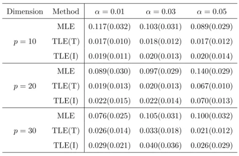
Table 4.1: Average (Std) of MCP, with n= 200. Dimension Method α= 0.01 α= 0.03 α= 0.05 MLE 0.117(0.032) 0.103(0.031) 0.089(0.029) p= 10 TLE(T) 0.017(0.010) 0.018(0.012) 0.017(0.012) TLE(I) 0.019(0.011) 0.020(0.013) 0.020(0.014) MLE 0.089(0.030) 0.097(0.029) 0.140(0.029) p= 20 TLE(T) 0.019(0.013) 0.020(0.013) 0.067(0.010) TLE(I) 0.022(0.015) 0.022(0.014) 0.070(0.013) MLE 0.076(0.025) 0.105(0.031) 0.100(0.032) p= 30 TLE(T) 0.026(0.014) 0.033(0.018) 0.021(0.012) TLE(I) 0.029(0.021) 0.040(0.036) 0.026(0.029)

4.2

Real data application

In this example, we consider applying both MLE and TLE of the mixture of factor analyzers to the wine data, which is available at the Machine Learning Repository of the University of California. The data set contains the results of chemical analysis of wines grown in the same region in Italy, but derived from three different cultivars. The analysis determined the quantities of p = 13 constituents found in each of n = 178 wines. Both MLE and TLE of the mixture of factor analyzers were fitted to this data set. Similar to the simulation study, the trimming proportion is set to be 0.05 for TLE.

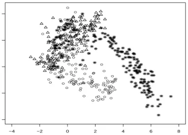
Based on McLachlan and Peel (2000), without the knowledge of true classification for parameters estimating, the error rate of the outright clustering is smallest forq= 2 and 3. In our analysis, q= 2 is used as our reduced dimension. Figure4.1 shows the values of sample means ˆµ_ij, the estimated posterior means of theq = 2 factors following a three-component mixture of factor analyzers of the wine data, which is actually the aij calculated from

E-step. These posterior means have been plotted with their true group labels corresponding to the three different cultivars displayed. From Figure4.1we can see that mixtures of factor analyzers have been useful here in exploring the grouping structure of the data in a much

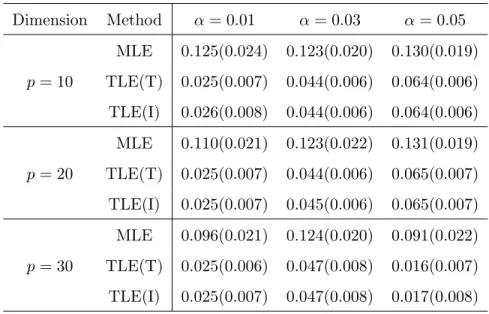
Table 4.2: Average (Std) of MCP, with n= 400. Dimension Method α= 0.01 α= 0.03 α= 0.05 MLE 0.125(0.024) 0.123(0.020) 0.130(0.019) p= 10 TLE(T) 0.025(0.007) 0.044(0.006) 0.064(0.006) TLE(I) 0.026(0.008) 0.044(0.006) 0.064(0.006) MLE 0.110(0.021) 0.123(0.022) 0.131(0.019) p= 20 TLE(T) 0.025(0.007) 0.044(0.006) 0.065(0.007) TLE(I) 0.025(0.007) 0.045(0.006) 0.065(0.007) MLE 0.096(0.021) 0.124(0.020) 0.091(0.022) p= 30 TLE(T) 0.025(0.006) 0.047(0.008) 0.016(0.007) TLE(I) 0.025(0.007) 0.047(0.008) 0.017(0.008) reduced dimension.

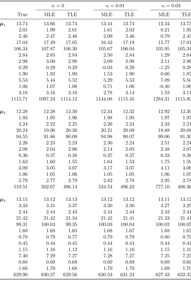
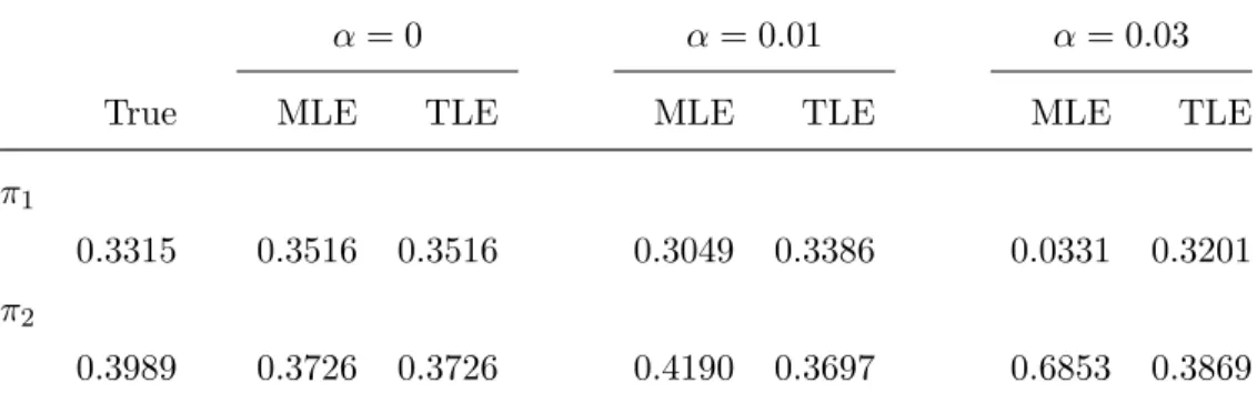
To assess the robustness of the two estimation methods, we also consider the contami-nated data by adding 1% and 3% outliers from U(9,11). Table 4.5 displays the estimated means µ₁, µ₂, and µ₃ via MLE and TLE when the proportion of outliers are α = 0, 0.01, and 0.03, and Table 4.6displays the estimated component proportions π1 and π2. The true

parameter values are calculated by using the true labels of observations. From both tables, we see that when there are no outliers, both MLE and TLE can provide comparatively good estimators. When the data is contaminated, however, TLE performs much better than M-LE. As the proportion of outliers gets higher, MLE departs further away from the original MLE without outliers, while TLE does not change much when the outliers are added to the data.

−4 −2 0 2 4 6 8 −6 −4 −2 0 2 ● ● ● ● ● ● ● ● ● ● ● ● ● ● ● ● ● ● ● ● ● ● ● ● ● ● ● ● ● ● ● ● ● ● ● ● ● _● ● ● ● ● ● ● ● ● ● ● ● ● ● ● ● ● ● ● ● ● ● ● ● ● ● ● ● ● ● ● ● ● ● ● ● ● ● ● ● ● ● ● ● ● ● ● ● ● ● ● ● ● ● ● ● ●● ● ● ● ● ● ● ● ● ● ● ● ● ● ● ● ● ● ●● ● ● ● ● ● ● ● ● ● ● ● ● ● ● ● ● ●● ● ● ● ● ● ● ● ●_● ● ● ● ● ● ● ● ● ● ● ● ● ● ● ● ● ● ● ● ● ● ● ● ● ● ● ● ● ● ● ● ● ● ● ● ● ●

Figure 4.1: Wine data: Plot of the estimated posterior means of the q = 2 factors (4, ◦, and ∗ denote true component membership).

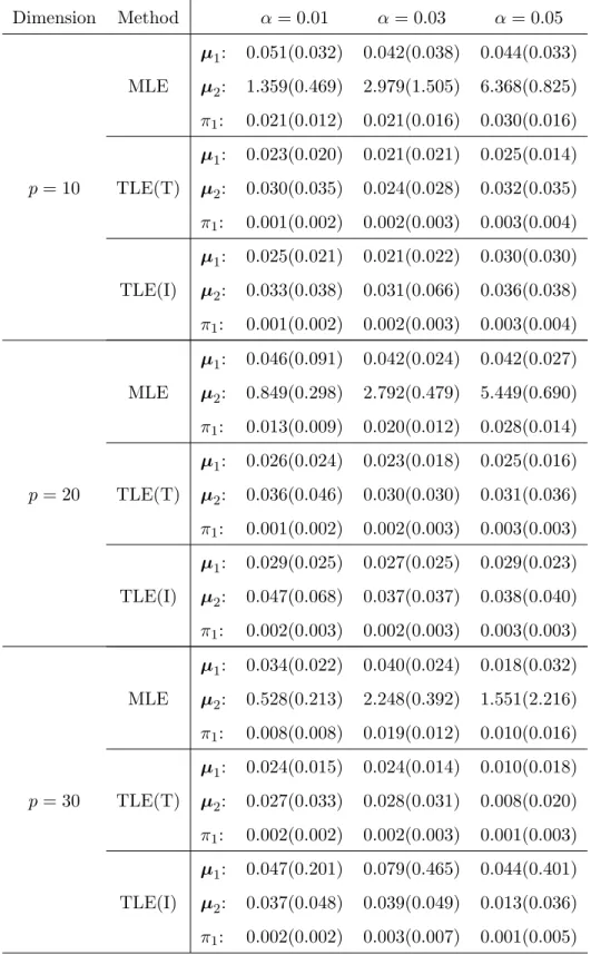
Table 4.3: Average (Std) of Euclidean distance, with n= 200. Dimension Method α= 0.01 α= 0.03 α= 0.05 µ₁: 0.051(0.032) 0.042(0.038) 0.044(0.033) MLE µ₂: 1.359(0.469) 2.979(1.505) 6.368(0.825) π1: 0.021(0.012) 0.021(0.016) 0.030(0.016) µ₁: 0.023(0.020) 0.021(0.021) 0.025(0.014) p= 10 TLE(T) µ₂: 0.030(0.035) 0.024(0.028) 0.032(0.035) π1: 0.001(0.002) 0.002(0.003) 0.003(0.004) µ₁: 0.025(0.021) 0.021(0.022) 0.030(0.030) TLE(I) µ₂: 0.033(0.038) 0.031(0.066) 0.036(0.038) π1: 0.001(0.002) 0.002(0.003) 0.003(0.004) µ₁: 0.046(0.091) 0.042(0.024) 0.042(0.027) MLE µ₂: 0.849(0.298) 2.792(0.479) 5.449(0.690) π1: 0.013(0.009) 0.020(0.012) 0.028(0.014) µ₁: 0.026(0.024) 0.023(0.018) 0.025(0.016) p= 20 TLE(T) µ₂: 0.036(0.046) 0.030(0.030) 0.031(0.036) π1: 0.001(0.002) 0.002(0.003) 0.003(0.003) µ₁: 0.029(0.025) 0.027(0.025) 0.029(0.023) TLE(I) µ₂: 0.047(0.068) 0.037(0.037) 0.038(0.040) π1: 0.002(0.003) 0.002(0.003) 0.003(0.003) µ₁: 0.034(0.022) 0.040(0.024) 0.018(0.032) MLE µ₂: 0.528(0.213) 2.248(0.392) 1.551(2.216) π1: 0.008(0.008) 0.019(0.012) 0.010(0.016) µ₁: 0.024(0.015) 0.024(0.014) 0.010(0.018) p= 30 TLE(T) µ₂: 0.027(0.033) 0.028(0.031) 0.008(0.020) π1: 0.002(0.002) 0.002(0.003) 0.001(0.003) µ₁: 0.047(0.201) 0.079(0.465) 0.044(0.401) TLE(I) µ₂: 0.037(0.048) 0.039(0.049) 0.013(0.036) π1: 0.002(0.002) 0.003(0.007) 0.001(0.005)

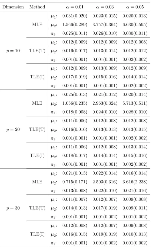
Table 4.4: Average (Std) of Euclidean distance, with n= 400. Dimension Method α= 0.01 α= 0.03 α= 0.05 µ₁: 0.031(0.020) 0.023(0.015) 0.020(0.013) MLE µ₂: 1.566(0.289) 3.757(0.364) 6.630(0.595) π1: 0.025(0.011) 0.026(0.010) 0.030(0.011) µ₁: 0.012(0.009) 0.012(0.009) 0.012(0.008) p= 10 TLE(T) µ₂: 0.016(0.017) 0.013(0.014) 0.012(0.012) π1: 0.001(0.001) 0.001(0.001) 0.002(0.002) µ₁: 0.012(0.009) 0.013(0.009) 0.012(0.009) TLE(I) µ₂: 0.017(0.019) 0.015(0.016) 0.014(0.014) π1: 0.001(0.001) 0.001(0.001) 0.002(0.002) µ₁: 0.025(0.013) 0.021(0.012) 0.020(0.014) MLE µ₂: 1.056(0.235) 2.963(0.324) 5.713(0.511) π1: 0.018(0.008) 0.024(0.010) 0.028(0.010) µ₁: 0.011(0.006) 0.012(0.008) 0.012(0.008) p= 20 TLE(T) µ₂: 0.016(0.016) 0.013(0.013) 0.013(0.015) π1: 0.001(0.001) 0.001(0.001) 0.002(0.002) µ₁: 0.011(0.006) 0.012(0.008) 0.013(0.014) TLE(I) µ₂: 0.018(0.017) 0.014(0.014) 0.015(0.016) π1: 0.001(0.001) 0.001(0.001) 0.002(0.002) µ₁: 0.021(0.013) 0.022(0.014) 0.016(0.014) MLE µ₂: 0.715(0.171) 2.503(0.316) 3.616(2.238) π1: 0.013(0.008) 0.022(0.010) 0.021(0.016) µ₁: 0.011(0.007) 0.012(0.007) 0.009(0.008) p= 30 TLE(T) µ₂: 0.014(0.013) 0.017(0.019) 0.009(0.011) π1: 0.001(0.001) 0.001(0.002) 0.001(0.002) µ₁: 0.012(0.008) 0.012(0.007) 0.009(0.008) TLE(I) µ₂: 0.016(0.015) 0.019(0.019) 0.010(0.013) π1: 0.001(0.001) 0.001(0.002) 0.001(0.002)

Table 4.5: Wine data: Estimated Means with α = 0,0.01, and 0.03. α = 0 α= 0.01 α= 0.03

True MLE TLE MLE TLE MLE TLE

µ₁ 13.74 13.66 13.74 13.44 13.74 12.34 13.73 2.01 1.99 2.01 1.61 2.02 0.21 1.99 2.46 2.47 2.46 2.09 2.46 0.79 2.43 17.04 17.49 17.05 16.42 17.18 15.77 17.01 106.34 107.87 106.30 105.67 106.04 105.95 105.34 2.84 2.85 2.84 2.50 2.84 1.29 2.84 2.98 3.00 2.98 2.69 2.98 2.11 2.96 0.29 0.29 0.29 -0.03 0.29 -1.25 0.28 1.90 1.92 1.90 1.53 1.90 0.66 1.87 5.53 5.44 5.52 5.29 5.53 7.09 5.50 1.06 1.07 1.06 0.71 1.06 -0.40 1.06 3.16 3.16 3.16 2.78 3.14 1.53 3.14 1115.71 1097.23 1114.12 1144.08 1115.45 1284.31 1115.80 µ₂ 12.28 12.28 12.30 12.34 12.32 12.92 12.30 1.93 1.95 1.96 1.98 1.95 1.97 1.97 2.24 2.22 2.25 2.26 2.24 2.33 2.24 20.24 19.96 20.26 20.21 20.09 18.88 20.08 94.55 91.86 90.09 94.98 90.07 99.06 91.30 2.26 2.23 2.23 2.30 2.24 2.51 2.24 2.08 2.04 2.06 2.14 2.05 2.48 2.07 0.36 0.37 0.38 0.37 0.37 0.33 0.38 1.63 1.60 1.55 1.64 1.53 1.75 1.59 3.09 3.05 3.07 3.17 3.07 4.11 3.06 1.06 1.05 1.06 1.05 1.05 1.06 1.05 2.79 2.77 2.79 2.82 2.78 2.95 2.78 519.51 502.67 496.14 534.54 496.23 777.10 498.36 µ₃ 13.15 13.12 13.13 13.12 13.12 13.11 13.12 3.33 3.31 3.37 3.30 3.30 3.27 3.29 2.44 2.44 2.43 2.44 2.44 2.43 2.44 21.42 21.42 21.34 21.42 21.41 21.33 21.41 99.31 100.03 99.35 100.03 100.04 100.02 100.05 1.68 1.68 1.65 1.68 1.67 1.68 1.67 0.78 0.79 0.77 0.79 0.79 0.80 0.79 0.45 0.44 0.45 0.44 0.44 0.44 0.44 1.15 1.16 1.12 1.16 1.16 1.15 1.16 7.40 7.29 7.27 7.28 7.27 7.25 7.25 0.68 0.69 0.69 0.69 0.69 0.69 0.69 1.68 1.70 1.68 1.70 1.70 1.69 1.70 629.90 630.27 629.56 630.53 631.24 627.43 632.32

Table 4.6: Wine data: Estimated component proportions with α= 0, 0.01, and 0.03. α= 0 α= 0.01 α= 0.03

True MLE TLE MLE TLE MLE TLE

π1

0.3315 0.3516 0.3516 0.3049 0.3386 0.0331 0.3201 π2

Chapter 5

Discussion

Mixtures of factor analyzers have been popularly used to do dimension reduction and model based clustering for high dimensional data. In this report, we investigate a robust estimation procedure of the mixtures of factor analyzers based on the TLE proposed by Neykov et al. (2007). The simulation study and real data analysis demonstrated the effectiveness of the TLE based robust estimation procedure.

In our examples, we have fixed the trimming proportion to be 0.05 for TLE. It works well whenever the true proportions of outliers are no more than 5%. However, it requires more research to find a data adaptive optimal or conservative trimming proportion for TLE in practice. Neykov et al. (2007) recommended a graphical tool to choose the trimming proportion in their examples. However, based on our limited empirical experience, such graphical tool was not very successful in choosing the trimming proportion for mixtures of factor analyzers. Therefore, we omitted the results in this report. There have been many methods proposed for choosing the trimming proportion for TLE in the non-mixture context. For example, Jure´ckov´a et al. (1994) studied the problem of choosing the trimming proportion for a trimmed L-estimator of location, and recommended the L-estimators with smooth weight functions. For the trimmed mean in the location modeling and for the trimmed least-squares estimator in the linear regression model, Dodge and Jure´ckov´a (1997) proposed a partially adaptive estimator of the trimming proportion based on a rank-based decision procedure. Clarke and Schubert (2010) studied an adaptive trimmed likelihood

estimator of regression, whose algorithm tends to expose the outliers automatically and provide the estimators with the outliers removed. It will be interesting to know whether we can extend the above methods to adaptively choose the trimming proportion for TLE in the mixture context.

Bibliography

[1] Andrews, J. L., McNicholas, P. D. and Subedi, S. (2011). Model-based classification via mixtures of multivariate t-distribution.Computational Statistics & Data Analysis, 55(1), 520-529.

[2] Arminger, G., Stein, P. and Wittenberg, J. (1999). Mixtures of conditional mean and covariance structure models. Psychometrika, 65, 475-494.

[3] Baek, J. and McLachlan, G. J. (2011). Mixtures of common t-factor analyzers for clustering high-dimensional microarray data. Oringnal Paper, 27(9), 1269-1276.

[4] Bishop, C. M. (1998). Latent variable models.Jordan, M.I. (Ed.), Learning in Graphical Models, pp, 371-403.

[5] Clark, B. R., Schubert, D. (2010). Adaptive trimmed likelihood estimation in regression. Probability and Statistics, 30, 203-219.

[6] Celeux, G., Hurn, M. and Robert, C. P. (2000). Computational and inferential difficul-ties with mixture posterior distributions. Journal of the American Statistical Associa-tion, 95, 957-970.

[7] Dodge, Yadolah and Jure´ckov´a (1997). Adaptive choice of proportion in trimmed least-squares estimation. Statistics & Probalility Letters, 33(2), 167-176.

[8] Fokou´e, E. and Titterington, D. M. (2003). Mixtures of factor analysers: Bayesian estimation and inference by stochastic simulation. Machine Learning, 50, 73-94.

[9] Ghahramani, Z. and Hinton, G. E. (1997). The EM algorithm for mixture of factor analyzers. University of Toronto Technical Report, CRG-TR-96-1.

[10] Gr¨un, B. and Leisch, F. (2009). Dealing with label switching in mixture models under genuine multimodality. Journal of Multivariate Analysis, 100, 851-861.

[11] Hinton, G. E., Dayan, P. and Revow, M. (1997). Modeling the manifolds of images of handwritten digits. IEEE Transaction, Neural Networks, 8, 65-73.

[12] Jasra, A, Holmes, C. C., and Stephens D. A. (2005). Markov chain Monte Carlo methods and the label switching problem in Bayesian mixture modeling.Statistical Science, 20, 50-67.

[13] Jure´ckov´a, J., Koenker, R., and Welsh, A. H. (1994). Adaptive choice of trimming proportions. Annals of the Institute of Statistical Mathematics, 46(4),737-755.

[15] McLachlan, G. J., Bean, R. W. and Ben-Tovim Jones, L. (2007). Extension of the mixture of factor analyzers model to incorporate the multivariatet−distribution. Com-putational Statistics & Data Analysis, 51, 5327-5338.

[15] McLachlan, G. J. and Peel, D. (2000). Finite mixture models. John Wiley & Sons, Inc, NY.

[16] McLachlan, G. J., Peel, D. and Bean, R. W. (2003). Modelling high-dimensional data by mixtures of factor analyzers.Computational Statistics&Data Analysis, 41, 379-388.

[17] Neykov, N., Filzmoser, P., Dimova, R. and Neytchev, P. (2007). Robust fitting of mix-tures using the trimmed likelihood estimator. Computational Statistics & Data Analy-sis, 52, 299-308.

[18] Neykov, N. M. and M¨uller, C. H. (2003), Breakdown points of the trimmed likelihood and related estimators in generalized linear models.Developments in Robust Statistics, pp, 277-286.

[19] Stephens, M. (2000). Dealing with label switching in mixture models. Journal of Royal Statistical Society, Ser B., 62, 795-809.

[20] Tipping, M. E., Bishop, C. M. (1997), Mixtures of probabilistic principal component analysers. Technical Report, No. NCRG/97/003, Neural Computing Research Group, Aston University, Birmingham

[21] Tipping, M. E. and Bishop, C. M. (1999). Mixtures of probabilistic principal component analysers. Neural Computation, 11, 443-482.

[22] Vandev, D. L. and Neykov, N. M. (1993). Robust maximum likelihood in the Gaussian case. New Directions in Data Analysis and Roubustness Morgenthaler, S., Ronchetti, E. and Stahel, W. A. (eds.), (Birkhauser Verlag, Basel, 1993)259-264.

[23] Wolberg, W. H. and Mangasarian, O. L. (1990). Multisurface method of pattern sep-aration for medical diagnosis applied to breast cytology. Proceedings of the National Academy of Sciences, 87, 9193-9196.

[25] Yao, W. (2012a). Model based labeling for mixture models. Statistics and Computing, 22, 337-347.

[25] Yao, W. (2012b). Bayesian mixture labeling and clustering. Communications in Statis-tics - Theory and Methods, 41, 403-421.

[26] Yao, W. (2013). A simple solution to Bayesian mixture labeling. Communication in Statistics–Simulation and Computation, 42, 800-813.

[27] Yao, W. and Lindsay, B. G. (2009). Bayesian mixture labeling by highest posterior density. Journal of American Statistical Association, 104, 758-767.

[28] Yung, Y. F. (1997). Finite mixtures in confirmatory factor analysis models. Psychome-trika, 62, 297-330.

Appendix A

R-Code

#define some necessary variables run=0;dif=10; n=dim(y)[2];p=dim(y)[1]; q=dim(lumbda1)[2] I<-diag(1,q) ezz1<-array(0,dim=c(q,q,n)) ezz2<-array(0,dim=c(q,q,n))

lh<-c() #lh records likelihood sequence repeat

run=run+1 lumbdaold1=lumbda1 lumbdaold2=lumbda2 # E step # generate expectation of pi sig1<-psi+lumbda1%*%t(lumbda1) sig2<-psi+lumbda2%*%t(lumbda2)

f1<-dmvnorm(t(y),mu1,sig1) #density function of component 1 f2<-dmvnorm(t(y),mu2,sig2) #density function of component 2 h1<-(pi1*f1)/(pi1*f1+pi2*f2) #expectation proportion 1 #h2<-(pi2*f2)/(pi1*f1+pi2*f2) #expectation proportion 2 h2=1-h1 if(min(sum(h1),sum(h2))<1){ ini=mfainitial(y,q,3*p); pi1=ini$pi1;pi2=ini$pi2;mu1=ini$mu1;mu2=ini$mu2; lumbda1=ini$lumbda1;lumbda2=ini$lumbda2;psi=ini$psi; out=mfa(y,pi1,pi2,mu1,mu2,lumbda1,lumbda2,psi,numrun) return(out) } lh[run]=sum(log(pi1*f1+pi2*f2))

# generate expectation of latent variable z

beta1<-t(lumbda1)%*%solve(psi+lumbda1%*%t(lumbda1)) beta2<-t(lumbda2)%*%solve(psi+lumbda2%*%t(lumbda2)) ez1<-beta1%*%(y-rep(mu1,n))

# generate expectation of z square for (i in 1:n){ ezz1[,,i]<-I-beta1%*%lumbda1+ez1[,i]%*%t(ez1[,i]) ezz2[,,i]<-I-beta2%*%lumbda2+ez2[,i]%*%t(ez2[,i]) } # M step # get new pi pi1<-sum(h1)/n pi2=1-pi1 #pi2<-sum(h2)/n

# get new miu

mu1<-t(h1%*%t((y-lumbda1%*%ez1)))%*%solve(sum(h1)) mu2<-t(h2%*%t((y-lumbda2%*%ez2)))%*%solve(sum(h2))

# get new lumbda sum1=0;sum2=0; for(i in 1:n){ sum1<-sum1+h1[i]*ezz1[,,i] sum2<-sum2+h2[i]*ezz2[,,i] } lumbda1<-((t(h1*t(y-rep(mu1,n))))%*%t(ez1))%*%solve(sum1) lumbda2<-((t(h2*t(y-rep(mu2,n))))%*%t(ez2))%*%solve(sum2)

psi<-(1/n)*diag(diag((t(h1*t(y-rep(mu1,n)-lumbda1%*%ez1)))%*%t(y-rep(mu1,n))+ (t(h2*t(y-rep(mu2,n)-lumbda2%*%ez2)))%*%t(y-rep(mu2,n))))

# give the rule to break

if(run>1){ dif=lh[run]-lh[run-1]} if(dif<0.001|run>numrun) {break} } out<-list(pi1=pi1,pi2=pi2,mu1=mu1,mu2=mu2,lumbda1=lumbda1,lumbda2=lumbda2,psi=psi,dif=dif,loglh=lh,posterior=cbind(h1,h2)) out } #############################

#Trimmed mixture of factor analyzers #########################

mfatrimone<-function(y,pi1,pi2,mu1,mu2,lumbda1,lumbda2,psi,alpha=0.95,numrun=500){ n=dim(y)[2];n1=round(n*alpha);

sig1<-psi+lumbda1%*%t(lumbda1) sig2<-psi+lumbda2%*%t(lumbda2)

f1<-dmvnorm(t(y),mu1,sig1) #density function of component 1 f2<-dmvnorm(t(y),mu2,sig2) #density function of component 2 lh=pi1*f1+pi2*f2 ind=order(-lh); run=0; acc=10^(-4); obj=sum(log(lh[ind[1:n1]])); repeat{ pobj=obj;run=run+1;indselected=ind[1:n1];

ynew=y[,indselected] out=mfa(ynew,pi1,pi2,mu1,mu2,lumbda1,lumbda2,psi); pi1=out$pi1;pi2=out$pi2;mu1=out$mu1;mu2=out$mu2; lumbda1=out$lumbda1;lumbda2=out$lumbda2;psi=out$psi; sig1<-psi+lumbda1%*%t(lumbda1) sig2<-psi+lumbda2%*%t(lumbda2)

f1<-dmvnorm(t(y),mu1,sig1) #density function of component 1 f2<-dmvnorm(t(y),mu2,sig2) #density function of component 2 lh=pi1*f1+pi2*f2 ind=order(-lh); obj=sum(log(lh[ind[1:n1]])); dif=obj-pobj; if(dif<0.001|run>numrun){break} } out$loglh=obj;out$dif=dif;out$ind=indselected;out$run=run out } mfainitial<-function(y,q,numsubset){ #q is the dimension latern variable. n=dim(y)[2];

p=dim(y)[1];

ind=sample(1:n,numsubset); sy=y[,ind];

hcTree=hc(modelName = "VII",data=t(sy)) #based on mclust cl=hclass(hcTree,2)

if(min(sum(cl==1),sum(cl==2))<2){ y1=sy[,1:round(numsubset/2)] y2=sy[,(round(numsubset/2)+1):numsubset] } else{ y1=sy[,cl==1] y2=sy[,cl==2] } if(min(sum(cl==1),sum(cl==2))>p){

out=factanal(t(y1),q) #based on factor analysis of stats

lumbda1=out$loadings; psi1=pmax(0.001,diag(cov(t(y1))-lumbda1%*%t(lumbda1))) out=factanal(t(y2),q) lumbda2=out$loadings; psi2=pmax(0.001,diag(cov(t(y2))-lumbda2%*%t(lumbda2))) psi=diag((psi1+psi2)/2) } else{ s1=cov(t(y1));psi1=diag(diag(s1)) cor1=cor(t(y1));eig=eigen(cor1) A1=eig$vectors[,1:q]; Lambda1=diag(pmax(eig$values[1:q],10^(-3))) sig1=mean(eig$values[(q+1):p]) lumbda1=psi1^(1/2)%*%A1%*%((Lambda1-sig1*diag(q))^(1/2))

s2=cov(t(y2));psi2=diag(diag(s2)) cor2=cor(t(y2));eig=eigen(cor2) A2=eig$vectors[,1:q]; Lambda2=diag(pmax(eig$values[1:q],10^(-3))) sig2=mean(eig$values[(q+1):p]) lumbda2=psi2^(1/2)%*%A2%*%((Lambda2-sig2*diag(q))^(1/2)) psi=(psi1+psi2)/2 } pi1=dim(y1)[2]/numsubset; pi2=1-pi1; mu1=rowMeans(y1); mu2=rowMeans(y2); out<-list(pi1=pi1,pi2=pi2,mu1=mu1,mu2=mu2,lumbda1=lumbda1,lumbda2=lumbda2,psi=psi) out } mfatrim<-function(y,q,alpha=0.95,numini=100,numrun1=50,numrun2=1000){ n=dim(y)[2]; p=dim(y)[1]; ini=mfainitial(y,q,n); pi1=ini$pi1;pi2=ini$pi2;mu1=ini$mu1;mu2=ini$mu2; lumbda1=ini$lumbda1;lumbda2=ini$lumbda2;psi=ini$psi; lh=rep(0,numini); est=mfatrimone(y,pi1,pi2,mu1,mu2,lumbda1,lumbda2,psi,alpha,numrun1);

lh[1]=est$loglh;

for(i in seq(numini-1)){ #print(i)

ini=mfainitial(y,q,min(round(n/2),3*p)); pi1=ini$pi1;pi2=ini$pi2;mu1=ini$mu1;mu2=ini$mu2; lumbda1=ini$lumbda1;lumbda2=ini$lumbda2;psi=ini$psi; temp=mfatrimone(y,pi1,pi2,mu1,mu2,lumbda1,lumbda2,psi,alpha,numrun1); lh[i+1]=temp$loglh; if(lh[i+1]>est$loglh){est=temp;} } pi1=est$pi1;pi2=est$pi2;mu1=est$mu1;mu2=est$mu2; lumbda1=est$lumbda1;lumbda2=est$lumbda2;psi=est$psi; est=mfatrimone(y,pi1,pi2,mu1,mu2,lumbda1,lumbda2,psi,alpha,numrun2); est$loglhseq=lh; est } posterior<-function(y,est){ pi1=est$pi1;pi2=est$pi2;mu1=est$mu1;mu2=est$mu2; lumbda1=est$lumbda1;lumbda2=est$lumbda2;psi=est$psi; sig1<-psi+lumbda1%*%t(lumbda1) sig2<-psi+lumbda2%*%t(lumbda2) f1<-dmvnorm(t(y),mu1,sig1) f2<-dmvnorm(t(y),mu2,sig2) h1<-(pi1*f1)/(pi1*f1+pi2*f2) h2=1-h1 out=cbind(h1,h2) out }

#####################Simulation study########## set.seed(10^8)

bt=Sys.time()

repnum=200; n=200; #n=200, n=400; q=2;p=10; #p=10; p=20

alpha=0.97 #trim proportion, alpha=0.95, alpha=0.97, alpha=0.99

numoutlier=round(n*(1-alpha))

#define sample sizes of two components pi1=0.4; pi2=1-pi1

#cprate is the classi

cprate=rep(0,n);cprate1=cprate;cprate2=cprate;cprate3=cprate; mse=matrix(rep(0,3*n),nrow=n);mse1=mse;mse2=mse;mse3=mse ### begin the replications

for(i in 17:repnum){ print(i) a<-rbinom(n,1,pi1) n1<-sum(a==1); n2<-n-n1

#define parameters pi,miu,lumbda and psi mu1=matrix(rep(0,p),p,1) mu2=matrix(rep(5,p),p,1) lumbda1<-matrix(rep(0.5,p*q),p,q) lumbda2<-matrix(rep(1,p*q),p,q) psi<-diag(p) #generate variable y z<-matrix(rnorm(n*q,mean=0,sd=1),q,n) e<-matrix(t(mvrnorm(n,rep(0,p),psi)),p,n) y1<-rep(mu1,n1)+lumbda1%*%z[,1:n1]+e[,1:n1]

y2<-rep(mu2,n2)+lumbda2%*%z[,(n1+1):n]+e[,(n1+1):n] y<-cbind(y1,y2) y[,1:numoutlier]=y[,1:numoutlier]-matrix(runif(numoutlier*p,20,30),nrow=p) trueposterior=matrix(c(rep(1,n1),rep(0,n2),rep(0,n1),rep(1,n2)),nrow=n) trueposterior=trueposterior[(numoutlier+1):n,]; out=mfa(y,pi1,pi2,mu1,mu2,lumbda1,lumbda2,psi,numrun=500) cp=out$posterior;cp=cp[(numoutlier+1):n,]; if(sum((cp>0.5)*trueposterior)>(n-numoutlier)/2){ cprate[i]=sum((cp>0.5)*trueposterior)/(n-numoutlier) mse[i,]=c(mean(out$mu1^2),mean((out$mu2-mu2)^2),(out$pi1-pi1)^2) } else{ cprate[i]=sum((cp>0.5)*(1-trueposterior))/(n-numoutlier) mse[i,]=c(mean(out$mu2^2),mean((out$mu1-mu2)^2),(out$pi2-pi1)^2) } out1=mfatrimone(y,pi1,pi2,mu1,mu2,lumbda1,lumbda2,psi,alpha=0.95,numrun=500) cp1=posterior(y[,(numoutlier+1):n],out1) if(sum((cp1>0.5)*trueposterior)>(n-numoutlier)/2){ cprate1[i]=sum((cp1>0.5)*trueposterior)/(n-numoutlier) mse1[i,]=c(mean(out1$mu1^2),mean((out1$mu2-mu2)^2),(out1$pi1-pi1)^2) } else{ cprate1[i]=sum((cp1>0.5)*(1-trueposterior))/(n-numoutlier) mse1[i,]=c(mean(out1$mu2^2),mean((out1$mu1-mu2)^2),(out1$pi2-pi1)^2) } out2=mfatrim(y,q,alpha=0.95,numini=20,numrun1=10,numrun2=500) if(out1$loglh>out2$loglh) out2=out1

cp2=posterior(y[,(numoutlier+1):n],out2) if(sum((cp2>0.5)*trueposterior)>(n-numoutlier)/2){ cprate2[i]=sum((cp2>0.5)*trueposterior)/(n-numoutlier) mse2[i,]=c(mean(out2$mu1^2),mean((out2$mu2-mu2)^2),(out2$pi1-pi1)^2) } else{ cprate2[i]=sum((cp2>0.5)*(1-trueposterior))/(n-numoutlier) mse2[i,]=c(mean(out2$mu2^2),mean((out2$mu1-mu2)^2),(out2$pi2-pi1)^2) } #out3=mvnormalmixEM(t(y),k=2,arbvar=1,maxit = 500) #cprate3[i]=sum((out3$posterior>0.5)*trueposterior) #if(sum((out3$posterior>0.5)*trueposterior)>n/2){ # cprate3[i]=sum((out3$posterior>0.5)*trueposterior)/n # mse3[i,]=c(mean(out3$mu[[1]]^2),mean((out3$mu[[2]]-mu2)^2),(out3$pi1-pi1)^2) #} #else{ # cprate3[i]=sum((out3$posterior>0.5)*(1-trueposterior))/n # mse3[i,]=c(mean(out3$mu[[2]]^2),mean((out3$mu[[1]]-mu2)^2),(out3$pi2-pi1)^2) #} } bt1=Sys.time()-bt save.image("E:\\Dropbox\\student\\liyang\\simulation\\ex-n200p30a99.RData") #load("E:\\Dropbox\\student\\liyang\\simulation\\ex-n400p20a95.RData") mean(cprate[1:repnum]) sqrt(var(cprate[1:repnum])) apply(mse[1:repnum,],2,mean)