Generative Modeling and Inference in Directed and Undirected Neural Networks

Undirected Neural Networks

Patrick Stinson

Submitted in partial fulfillment of the requirements for the degree

of Doctor of Philosophy under the Executive Committee of the Graduate School of Arts and Sciences

COLUMBIA UNIVERSITY

Generative Modeling and Inference in Directed and

Undirected Neural Networks

Patrick Stinson

Generative modeling and inference are two broad categories in unsupervised learning whose goal is to answer the following questions, respectively: 1. Given a dataset, how do we (either implicitly or explicitly) model the underlying probability distribution from which the data came and draw samples from that distribution? 2. How can we learn an underlying abstract representation of the data? In this dissertation we provide three studies that each in a different way improve upon specific generative modeling and inference techniques. First, we develop a state-of-the-art estimator of a generic probability distribution’s partition function, or normalizing constant, during simulated tempering. We then apply our estimator to the specific case of training undirected probabilistic graphical models and find our method able to track log-likelihoods during training at essentially no extra computational cost. We then shift our focus to variational inference in directed probabilistic graphical models (Bayesian networks) for generative modeling and inference. First, we generalize the aggregate prior distribution to decouple the variational and generative models to provide the model with greater flexibility and find improvements in the model’s log-likelihood of test data as well as a better latent representation. Finally, we study the variational loss function and argue under a typical architecture the data-dependent term of the gradient decays to zero as the latent space dimensionality increases. We use this result to propose a simple modification to random weight initialization and show in certain models the modification gives rise to substantial improvement in training convergence time. Together, these results improve quantitative performance of popular generative modeling and inference models in addition to furthering our understanding of them.

List of Figures iv

List of Tables vii

Chapter 1 Introduction 1

1.1 Overview . . . 1

1.2 Monte Carlo methods . . . 3

1.3 Latent variable modeling . . . 7

1.4 Variational inference . . . 8

1.5 Undirected models . . . 9

Chapter 2 Partition functions from Rao-Blackwellized tempered sampling 11 2.1 Introduction . . . 12

2.2 Partition functions from tempered samples . . . 13

2.2.1 Simulated tempering . . . 14

2.2.2 Estimating partition functions . . . 15

2.2.3 Rao-Blackwellized likelihood interpretation . . . 16

2.2.4 Initial iterations . . . 19

2.2.5 Bias and variance . . . 20

2.3 Related work . . . 21 2.3.1 Wang-Landau . . . 21 2.3.2 AIS/RAISE . . . 21 2.3.3 BAR/MBAR . . . 22 2.3.4 Thermodynamic integration . . . 24 2.4 Examples . . . 25 i

2.4.3 Number of temperatures . . . 28

2.4.4 Tracking partition functions while training . . . 29

2.5 Discussion . . . 31

Chapter 3 Decoupling aggregate priors in variational autoencoders 33 3.1 Introduction . . . 34

3.2 Variational Autoencoders . . . 36

3.3 Prior Choice . . . 37

3.3.1 Aggregate priors . . . 37

3.3.2 Decoupling . . . 39

3.3.3 Connection with kernel density estimation . . . 40

3.4 Experiments . . . 42

3.5 Conclusion . . . 45

Chapter 4 ELBO amputation: an initialization scheme for variational autoen-coders 48 4.1 Introduction . . . 48

4.2 ELBO gradients . . . 50

4.2.1 Cross-covariance interpretation of gradient . . . 51

4.2.2 Potential concerns: code collapse and symmetry . . . 53

4.2.3 Numerical simulation . . . 53

4.2.4 Application to sequential autoencoder . . . 54

4.3 Discussion . . . 56

Chapter 5 Conclusion 59 Bibliography 61 Appendix A Chapter 2 Appendix 69 A.1 Estimatingq(βk) from a transition matrix . . . 69

A.4 RTS and TI-RB Continuousβ Equivalence . . . 75

Appendix B Chapter 4 Appendix 78 B.1 Linear function . . . 79

B.2 Linear + ReLU function . . . 79

B.3 Linear + ReLU layer . . . 82

B.4 Linear + ReLU network . . . 83

Appendix C Gaussian tube prior 85 C.1 Examining latent space . . . 86

Appendix D Flow-based prior 89 D.1 Flow-based prior . . . 90

Figure 2.1 Comparison of log ˆZkand log ˆckestimates, in some of the first eight iterations

of the initialization procedure described in Section 2.2.4, with and without Rao-Blackwellization, with K = 100. The initial values were ˆZk = 1 for all k, and

the prior was uniform, rk = 1/K. The model is a RBM with 784 visible and 10

hidden units, trained on the MNIST dataset. Each iteration consists of 50 Gibbs sweeps, on each of 100 parallel chains. Since in the non-Rao-Blackwellized case, the updates are unstable and sometimes infinite, for demonstration purposes only, we define ˆck ∝ 0.1 +PN_i=1δk,k(i) and normalize. Note that in the Rao-Blackwellized

case, the values of ˆckin the final iteration are very close to those ofrk, signaling that

the ˆZk’s are good enough for a last, long MCMC run to obtain the final ˆZkestimates. 17

Figure 2.2 Comparison of logZ estimation performance on a toy Gaussian Mixture Model using an RMSE from 10 repeats. TI Riemann approximates the discrete integral as a right Riemann sum, TI trap uses the trapezoidal method, TI trap corrected uses a variance correction technique, TI RB uses the Rao-Blackwellized version of TI. . . 26 Figure 2.3 Mean and root mean squared error (RMSE) of competing estimators of logZK

evaluated on RBMs with 784 visible units trained on the MNIST dataset. The numbers of hidden units were 500 (Top) and 100 (Bottom). In both cases, the bias from RTS decreases quicker than that of AIS and RAISE, and the RMSE of AIS does not approach that of RTS at 1000 Gibbs sweeps until over an order of magnitude later. Each method is run on 100 parallel Gibbs chains, but the Gibbs sweeps in the horizontal axis corresponds to each individual chain. . . 27

Each point was obtained by averaging over 200 estimates (20 for MBAR due to computational costs) made from 10,000 bootstrapped samples from a long MCMC run of 3 million samples. . . 29 Figure 2.5 A demonstration of the ability to track with minimal cost the mean train and

validation log-likelihood during the training of a RBM on the dna 180-dimensional binary dataset, with 500 latent features. . . 31

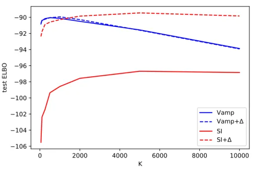
Figure 3.1 Proposed aggregate decoupling model. The vanilla aggregate prior is shown in black and is unchanged; u can represent either pseudoinputs or random data subsamples. Decoupling via the delta function/network is shown in gray and dotted lines. . . 40 Figure 3.2 Test ELBO terms as a function ofK (static MNIST). . . 45 Figure 3.3 ELBO terms as a function of K (static MNIST): (a) test reconstruction

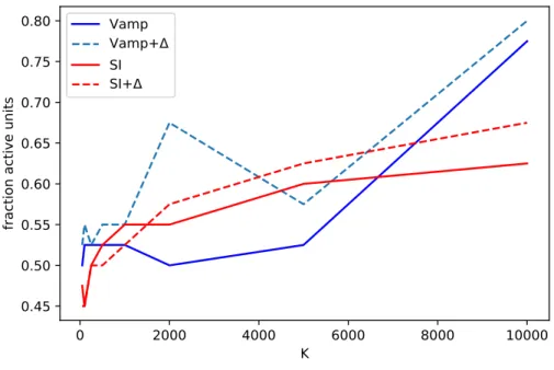
log-probability, (b) test KL(q(z)||p(z)). Asterisks indicate the values of K which maximize the test ELBO for each model in (a) and (b). . . 46 Figure 3.4 Fraction of active latent units for each model as a function ofK. . . 47

Figure 4.1 Closed-form KL gradients dominate during the beginning of training. Top: Cosine similarity between MCMC estimated µ gradient for and closed-form µ KL gradient during training. Middle: Same for λ gradients. Bottom: ELBO during training. . . 57 Figure 4.2 Training a sequential autoencoder on MNIST. Comparison of test ELBOs

during training between zero initialization and (a) standard initialization (b) various KL annealing schedules. The length of annealing in iterations for each schedule is written after ‘anneal’ in the legend. . . 58

Experimental procedure is the same as the main text. (Left) RTS, TM, and RTM compared on a 784-10 RBM. Because the latent dimensionality is small, mixing is very effective and accounting for the transition matrix improves performance consis-tently by about 10%. (Right) For an 784-200 RBM, the approximation as a Markov transition is inaccurate, and we observe no performance improvements. . . 71 Figure A.2 (Left) Mixing inβ under the fixed step size. (Center) Mixing in β under the

adaptive scheme. (Right) Partition function estimates under the fixed step size and adaptive scheme after 10000 samples. Mixing in β using a fixed step size is visibly slower than mixing using the adaptive step size, which is reflected by the error in the partition function estimate. . . 73

Figure C.1 Interpolating position. Top-left: standard normal prior,top-right VampPrior, bottom-left: SI prior, bottom-right: Gaussian tube. . . 87 Figure C.2 Interpolating size. Top-left: standard normal prior, top-right VampPrior,

bottom-left: SI prior, bottom-right: Gaussian tube. . . 87

Table 3.1 Test log-likelihoods on three data sets. . . 44

I first would like to thank my advisor Liam Paninski. When I joined the group, I was amazed by the degree of engagement you had in my projects–it’s astounding to me that despite the large volume of research being done in the group you are not only able to keep abreast of the technical details but also contribute a steady stream of original ideas.

I would also like to thank the members of my thesis committee: Niko Kriegeskorte, Larry Ab-bott, John Cunningham, and Rajesh Ranganath. You were instrumental in supporting a direction for me to take to finish. I would like to thank Niko in particular not only for chairing the committee but also for inspiring me with your far-reaching curiosity, positive attitude, and encouragement.

I would like to thank Leslie Osborne for her confidence in me. It was only after an introduction to information theory and those fly papers that my interest in machine learning started to take off. I thank Jason Maclean for inspiring me ultimately to take the plunge and attend graduate school. I admired your no nonsense approach to research and the lab environment you cultivated during my time at UChicago. You and your students treated me like one of your own.

I would also like to thank my friends. Dan, for the gym celebrity tiers and Ganon v. Ganon matches. Uygar, for the nights working together in the office. Xuexin, for your enthusiasm for conversation and great generosity with your time. Kenny, for our philosophical conversations that stop time for hours. Erdem, for a friendship that would make Zizek blush. Cat, for countless conversations and schemes.

Finally, I thank Audrey for all of her love, companionship, and support.

Chapter 1

Introduction

“We are forced to tell the truth, we are constrained, we are condemned to admit the truth or

to discover it.” — Michel Foucault

1.1

Overview

Much of what is commonly thought of as cognition can be considered a form of inference; it is

usually not the data itself that we care about or even seem to think about but rather a more abstract

form of the data. Instead of perceiving the world as streams of ‘raw’ data from our sensory faculties,

we cut through redundancy and nuisance by perceiving on a more general and abstract level: we

see objects that belong to various conceptual hierarchies, we hear words and sentences instead of

phonemes, etc. Inference takes place at every level of complexity of life, from axonal growth cones

inferring directions of chemical gradients from the stochastic pattern of receptors binding to the

chemical molecules [Mortimer et al., 2009], to the mind’s abstraction of concepts [Tenenbaum et al.,

2011], to global inference emergent in message passing across networks of individuals (see e.g., [Xu

et al., 2014; Vehtari et al., 2014] for how this could be realized in a computational framework).

is closely tied to inference. In many frameworks, they are learned simultaneously. Intuitively, having

a good model of the important abstract elements of the data should make it easier to generate data

that contain these elements. In other words, it’s easier to draw a chair when you know what a chair

is.

Generative modeling provides a means of general-purpose data augmentation whose

impor-tance may soon come to the forefront of research as more sophisticated models require more data,

but there is a more ambitious goal hidden in the form of a sanity check. If we are able to learn

from a dataset to in turn generate data that exhibit characteristics from that dataset, our model

may have captured in some form the causal factors that gave rise to the data in our dataset. More

succinctly, in the limit that our generative model can produce arbitrarily accurate and diverse

samples from a distribution, the model has captured all the information in that distribution.

The contributions in this thesis to generative modeling and inference are as follows: in

Chapter 2, we develop a method to estimate partition functions of hard to sample

distribu-tions, which we use to improve training of Restricted Boltzmann Machines [Smolensky, 1986].

In Chapters 3 and 4, we shift our focus to variational autoencoders [Kingma and Welling, 2014;

D.J. Rezende, 2014]. In Chapter 3, we decouple the inference and generative models by

gener-alizing the prior distribution and improve performance. In Chapter 4, we show that a simple

random weight initialization modification can lead to substantial training improvements for VAEs

with large latent dimension. We conclude with a discussion in Chapter 5. To improve the flow of

the thesis, more dense mathematical work for Chapters 2 and 4 has been moved to Appendices

A and B, respectively. We include some negative results in Appendices C and D that the reader

can omit without detriment to the rest of the thesis. For the remainder of this chapter, we

pro-vide the background necessary for easy reading of these chapters in an effort to make this work

1.2

Monte Carlo methods

Monte Carlo methods [Robert and Casella, 2013] comprise a general purpose toolbox for

estimating expectations over arbitrary (with mild restrictions) probability distributions. As we will

see, essentially all of the quantities we are interested in take the form of expectations, so their

utility cannot be overstated.

Suppose we have a function f(x) that we would like to average over some probability

dis-tribution p(x). Ignoring mild restrictions on f(_·) and p(_·), the strong law of large numbers tells us 1 N N X n=1 f(x(n))_−−→a.s. Ep(x)[f(x)], (1.1) wherex(n) _∼p(·).

In other words, we can estimate the average of a function of a random variable by simply

averaging function evaluations at random samples. Importantly, if we take an expectation over the

left hand side of (1.1), we see that our estimate is unbiased; that is, E[E\[f(x)]] =E[f(x)].

(1.1) applies so long as we can easily sample from p(_·). If p(_·) isn’t easy to sample from, we can still make use of (1.1) with a little extra work.

One option is rejection sampling. If we pick an easy to sample from distributionq(x) and can

boundp(x)/q(x) byM <∞, rejection sampling is done by following Algorithm 1.

The issue with rejection sampling is that M must be picked beforehand and cannot be

arbi-trarily large since

P(accept) =Eq p(x) M q(x) = 1 M.

Since M is hard to pick for high dimensional distributions, rejection sampling is usually

Algorithm 1 Rejection Sampling initialize s= 1 while s_≤S do Samplex_∼q(_·) and u_∼U[0,1]. if u > _{M q}p(x_(x)₎ then x(s)_=x s=s+ 1 end if end while return_{x(s)_}S s=1

A second option is importance sampling, which we can derive by noting

Ep[f(x)] = Z f(x)p(x)dx (1.2) = Z f(x)p(x)q(x) q(x)dx (1.3) = Z f(x)p(x) q(x)q(x)dx (1.4) =Eq[w(x)f(x)], (1.5)

where q(x) is called the importance distribution and w(x) = _qp(₍x_x)₎ are the importance weights. If q(x) is easy to sample from, we can just sample from it and weight our evaluations of f(x) with

x∼q(·) by w(x).

A potential problem with importance sampling, however, is if q(_·) does not match well with p(_·) on some subset of p’s support. Intuitively, if there are regions where q(x) is small but p(x) is large, or vice versa, the importance weights will be relatively high or low, respectively. The result is

high variance importance weights and consequently a high variance Monte Carlo estimate. As with

rejection sampling, high dimensional probability distributions often preclude importance sampling,

since the probability of such regions existing is high.

sampling by exploring the space of x _{∈ X} based on a series of jumps. By doing so, we trade off having to find a suitable distribution q(·) to match p(·) globally with introducing temporal correlations between samples.

A Markov Chain is a sequencex(1)_{, x}(2)_{, ..., x}(N) _{whose dynamics obey the following identity}

p(x(i)) =T(x(i)_|x(i−1)), (1.6) where T(x(i)_|x(i−1)_{) is called the transition function. To start the chain, x}

0 ∼ p0(x) must be

specified.

A distribution p(x) is said to be the invariant distribution of the Markov Chain specified by

T(_·|·) if

lim

N→∞P(x

(N)_|x(N) _{=x) =p(x). (1.7)}

That is, we can draw samples whose distribution is arbitrarily close to p(x) by running the

Markov Chain for enough steps. For any x0, it can be shown that if T(x(i)|x(i−1)) is irreducible

(T(x(i)_|x(j)_{) > 0 for all i, j) and aperiodic (it does not get stuck in cycles), the Markov Chain}

will converge to the invariant distribution. Note in the discrete case, running a Markov Chain is

equivalent to a power iteration; consequently, we can conclude that the first eigenvector ofT is the

invariant distribution p(x) (for continuous distributions, it is the first eigenfunction).

Most of the time though, we are interested in deriving a transition function from a desired

invariant distribution–not the other way around. The condition of detailed balance provides a

sufficient but not necessary condition for a transition function to have an invariant distribution

p(x):

p(x(i))T(x(i−1)_|x(i)) =p(x(i−1))T(x(i)_|x(i−1)). (1.8) The Metropolis-Hastings algorithm [Metropolis et al., 1953] is derived from satisfying detailed

function

T(x(i)_|x(i−1)) =A(x(i)_|x(i−1))g(x(i)_|x(i−1)) + (1₋A(x(i)_|x(i−1)))δ(x(i−1)), (1.9) for some proposal distributiong(·|·) whereA(x(i)_|x(i−1)_{) = min1,} p(x(i))g(x(i−1)|x(i))

p(x(i−1)_)g(x(i)_|x(i−1)₎

.

Note that multiplyingp(x) by a constant does not affect the transition function in (1.9), which

enables us to sample from unnormalized distributions.

As a special case, consider the proposal distribution g(x(i)_|x(i−1)_{) = δx}(i)

−j =x

(i−1)

−j

+

p(xj|x−(ij−1)), where x−j , x\xj, called Gibbs sampling [Geman and Geman, 1984]. It is easily

shown the probability of accepting a proposal from a conditional distribution ofp(x) is 1.

A common choice for the proposal distribution is a symmetric Gaussian g(x(i)_|x(i−1)_{) =}

N(x(i)_{|0,Σ). Note, however, that Σ may not be easy to determine and for certain distributions a}

static transition matrix will lead to poor mixing, the time taken such that a sample from the chain

is approximately from the invariant distribution. For example, consider a mixture of two isotropic

Gaussians with one component having a large variance and the other having a small variance. If Σ

is large, if we are within the flatter component, we will have good mixing, but when we transition

to the sharper component, it will be difficult to accept the large jumping proposals, since we are

already in a high density region. Conversely, if we have a small Σ, we will be able to move in the

sharper component, but movement in the flatter component will be relatively slow.

As the target distribution becomes more difficult to sample from, these simpler methods will no

longer be sufficient. We will see examples of more sophisticated methods later, including simulated

1.3

Latent variable modeling

If we believe our data can be described in terms of more abstract but less complicated factors,

instead of directly modeling how the data behave, we can instead model how the so-called latent

variables behave and how the latent variables influence the data. The utility of such modeling is

twofold: we build a probabilistic model of the data, but given a data point, we can also infer (or

approximate) the distribution of the underlying latent variables that gave rise to the data point.

Factor analysis [Cattell, 1952] models the data as the sum of linear projections from latent

factors. The simplest case is linear Gaussian factor analysis, in which

p(z) =_N(z_|0, I) (1.10)

p(x|z) =N(x|µ+ Λz,Σ), (1.11) where x represents our data and z represents our latent variables. To fit this model to the data,

we can perform Expectation Maximization (EM) [Dempster et al., 1977].

This simple mixing model has substantial limitations. In particular, the additivity of latent

factors restricts the expressiveness of the model, causing Gaussian mixture models to tend to

oversmooth. If we deviate much from the Gaussian mixture model, though, we can no longer do

EM, as we can no longer evaluate the posterior distribution, since it requires marginalization over

the latents: p(z_|x) = p(x, z) p(x) = p(x, z) R p(x, z)dz, (1.12)

which cannot be evaluated in many (non-conjugate) models.

We will explore two alternatives: 1. using a generalization of EM called variational inference

[Jordan et al., 1999] to train models in which the posterior cannot be evaluated 2. using an

1.4

Variational inference

Suppose we take our factor analysis model in the previous section and after taking an affine

transformation of the factors, we compose the transformation with a nonlinear function f(·) and definex|z∼p(x;θ=f(W z+b)), wherepis some density with parametersθ. f(·) induces coupling between the latent variables, which we can see by taking a Taylor expansion of some element of

f(z), fi(z), atz0: fi(z) =fi(z0) +∇fi(z0)T(z−z0) + 1 2(z−z0) T_∇2_f i(z0)(z−z0) +· · ·. (1.13)

The nonlinear coupling of latent variables endows the model with a great amount of flexibility,

enabling the latent variables to represent distinct features of the data. Additionally, since the

composition of two nonlinear functions does not reduce in the same way that linear functions do,

we can add more latent variables to the model and ‘stack’ layers such that, e.g., p(x) = p(x_|θ = f(W(1)_z(1) _+b(1)_{)) and p(z}(1)_{) = p(z}(1)_{|θ = f(W}(0)_z(0)_+b(0)_{). The price we must pay for this}

flexibility is thatp(z_|x) is no longer tractable.

Instead, variational inference (VI) [Jordan et al., 1999] introduces a variational distributionq(_·) to approximate the posterior distribution and maximizes a lower bound on the evidence (ELBO):

L(x) =Eq(z)[logp(x, z)−logq(z)]. (1.14)

It turns out that the gap between the ELBO and the evidence is the KL-divergence between

the variational distribution and the true posterior:

logp(x) = Z logp(x)q(z)dz = Z [logp(x, z)−logp(z|x)]q(z)dz = Z

[logp(x, z)₋logq(z) + logq(z)₋logp(z_|x)]q(z)dz

If the variational distribution takes a particular form, such as a mean-field distributionq(z) = Q

iqi(z) and qi(·) is in the exponential family, coordinate ascent methods to optimize each qi(·)

individually can be performed. However, this can place a large constraint on the family of variational

distributions available, potentially increasing the gap between the ELBO and the evidence.

We can improve the variational distribution’s flexibility by amortizingq(z) and turning it into

a function of x, q(z_|x), and optimizing the ELBO through stochastic gradient descent [Bottou, 2010]. However, the training gradient from these estimates can be relatively noisy, often requiring

design of control variates [Mnih and Gregor, 2014; Mnih and Rezende, 2016] to reduce the noise.

We can substantially reduce the noise in the ELBO gradient making use of the

‘reparameter-ization trick’ in variational autoencoders [Kingma and Welling, 2014; D.J. Rezende, 2014]. When

the stochastic latent variable comes from a distribution that can be reparameterized as a

func-tion of parameterless ‘base’ distribufunc-tion and parameters of the original latent distribufunc-tion (e.g.,

z _{∼ N}(µ, σ2_{) = σ∗+µ, ∼ N(0, I)), we can express the ELBO gradient in terms of the latent}

parameters, which often greatly reduces its variance. This, however, constrains our latent variables

to come from a class of parametric models.

1.5

Undirected models

An alternative to variational inference in directed models is the undirected energy-based model,

in which inference is exact and easy, but sampling (which is exact and easy in directed models) is

difficult.

The density of an energy-based model takes the form

p(x, z) = 1

Z exp(−E(x, z)), (1.16)

Note that we do not have to specify a prior distribution on the latents, in contrast to Factor

Analysis and the directed model we will use for the variational autoencoder. It is tempting to view

the prior distribution as trivial; however, we will see in Chapter 3 that this is the fundamental

‘issue’ with the autoencoder.

In Chapter 2, we will train the Restricted Boltzmann Machine whose energy function takes

the form

ERBM(x, z) =−aTx−bTz−xTW z. (1.17)

Evaluating the conditional distributions p(x|z) andp(z|x) is easy in this model. To perform infer-ence, a simple calculation gives

p(z|x) = P Y i=1 p(zi|x) = P Y i=1 σ(ai+WiTz), (1.18)

whereσ(_·) is the sigmoid function σ(x), _1+exp(1 −x).

The downside to this model is that it is very difficult to produce samples from the model. In

contrast to directed models, in which one simply samples from the prior distribution over latent

variables and performs a single feedfoward pass to sample x, in the RBM, one must perform

(blockwise) Gibbs sampling by starting at some initial configurationx(0)_{and alternatively sampling}

z(0) _{∼ p(z|x}(0)_{), x}(1) _{∼ p(x|z}(0)_{), z}(1) _{∼ p(z|x}(1)_{), ..., x}(N) _{∼ p(x|z}(N−1)_{), where N can be of}

the order of 105 _{to achieve proper burn-in [Salakhutdinov, 2010]. Since sampling from p(x) is}

difficult, training has traditionally been done with approximate maximum likelihood methods, e.g,

contrastive divergence [Hinton, 2002], which truncate the chain before it has reached convergence

Chapter 2

Partition functions from

Rao-Blackwellized tempered sampling

David Carlson*, Patrick Stinson*, Ari Pakman*, Liam Paninski, ICML 2015

(*equal contribution)

Partition functions of probability distributions are important quantities for model

evalua-tion and comparisons. We present a new method to compute partievalua-tion funcevalua-tions of complex and

multimodal distributions. Such distributions are often sampled using simulated tempering, which

augments the target space with an auxiliary inverse temperature variable. Our method exploits

the multinomial probability law of the inverse temperatures, and provides estimates of the

par-tition function in terms of a simple quotient of Rao-Blackwellized marginal inverse temperature

probability estimates, which are updated while sampling. We show that the method has interesting

connections with several alternative popular methods, and offers some significant advantages. In

particular, we empirically find that the new method provides more accurate estimates than

Machines (RBM); moreover, the method is sufficiently accurate to track training and validation

log-likelihoods during learning of RBMs, at minimal computational cost.

2.1

Introduction

The computation of partition functions (or equivalently, normalizing constants) and marginal

likelihoods is an important problem in machine learning, statistics and statistical physics, and is

necessary in tasks such as evaluating the test likelihood of complex generative models, calculating

Bayes factors, or computing differences in free energies. There exists a vast literature exploring

methods to perform such computations, and the popularity and usefulness of different methods

change across different communities and domain applications. Classic and recent reviews include

[Gelman and Meng, 1998; Vyshemirsky and Girolami, 2008; Marin and Robert, 2009; Friel and

Wyse, 2012].

In this paper we are interested in the particularly challenging case of highly multimodal

dis-tributions, such as those common in machine learning applications [Salakhutdinov and Murray,

2008]. Our major novel insight is that simulated tempering, a popular approach for sampling from

such distributions, also provides an essentially cost-free way to estimate the partition function.

Simulated tempering allows sampling of multimodal distributions by augmenting the target space

with a random inverse temperature variable and introducing a series of tempered distributions.

The idea is that the fast MCMC mixing at low inverse temperatures allows the Markov chain to

land in different modes of the low-temperature distribution of interest [Marinari and Parisi, 1992;

Geyer and Thompson, 1995].

As it turns out, (ratios of) partition functions have a simple expression in terms of ratios of

the parameters of the multinomial probability law of the inverse temperatures. These parameters

along the Markov chain. This simple method matches state-of-the-art performance with minimal

computational and storage overhead. Since our estimator is based on Rao-Blackwellized marginal

probability estimates of the inverse temperature variable, we denote it Rao-Blackwellized Tempered

Sampling (RTS).

In Section 2.2 we review the simulated tempering technique and introduce the new RTS

estimation method. In Section 2.3, we compare RTS to Annealed Importance Sampling (AIS) and

Reverse Annealed Importance Sampling (RAISE) [Neal, 2001; Burda et al., 2015], two popular

methods in the machine learning community. We also show that RTS has a close relationship with

Multistate Bennett Acceptance Ratio (MBAR) [Shirts and Chodera, 2008; Liu et al., 2015] and

Thermodynamic Integration (TI) [Gelman and Meng, 1998], two methods popular in the chemical

physics and statistics communities, respectively. In Section 2.4, we illustrate our method in a simple

Gaussian example and in a Restricted Boltzmann Machine (RBM), where it is shown that RTS

clearly dominates over the AIS/RAISE approach. We also show that RTS is sufficiently accurate to

track training and validation log-likelihoods of RBMs during learning, at minimal computational

cost. We conclude in Section 2.5.

2.2

Partition functions from tempered samples

In this section, we start by reviewing the tempered sampling approach. We then introduce our

procedure to estimate partition functions by tempered sampling. We note here that our approach

is useful not only as a stand-alone method for estimating partition functions, but is also essentially

2.2.1 Simulated tempering

Consider an unnormalized, possibly multimodal distribution proportional tof(x), whose

par-tition function we want to compute. Our method is based on simulated tempering, a well known

approach to sampling multimodal distributions [Marinari and Parisi, 1992; Geyer and Thompson,

1995]. Simulated tempering begins with a normalized and easy-to-sample distribution p1(x) and

augments the target distribution with a set of discrete inverse temperatures {0 = β1 < β2 < ... <

βK = 1}to create a series of intermediate distributions betweenf(x) and p1(x), given by

p(x_|βk) = fk(x) Zk , (2.1) where fk(x) =f(x)βkp1(x)1−βk, (2.2) and Zk= Z fk(x)dx . (2.3)

ZK is the normalizing constant that we want to compute. Note that we assume Z1 = 1 and

p(x_|β1) = p1(x). However, our method does not depend on this assumption. When performing

model comparison through likelihood ratios or Bayes factors, both distributionsf(x) andp1(x) can

be unnormalized, and one is interested in the ratio of their partition functions. For the sake of

simplicity, we consider here only the interpolating family given in (2.2); other possibilities can be

used for particular distributions, such as moment averaging [Grosse et al., 2013] or tempering by

subsampling [van de Meent et al., 2014].

r(βk) =rk, and define the joint distribution

p(x, βk) =p(x|βk)rk (2.4)

= fk(x)rk Zk

, (2.5)

whereZk is unknown. Instead, suppose we know approximate values ˆZk. Then we can define

q(x, βk)∝

fk(x)rk

ˆ Zk

, (2.6)

which approximatesp(x, βk). We note that the distributionq depends explicitly on the parameters

ˆ

Zk. A Gibbs sampler is run on this distribution by alternating between samples fromx|β andβ|x.

In particular, the latter is given by

q(βk|x) =

fk(x)rk/Zˆk

PK

k0₌₁f_k0(x)r_k0/Zˆ_k0

. (2.7)

Sampling as such enables the chain to traverse the inverse temperature ladder stochastically,

es-caping local modes under low β and collecting samples from the target distribution f(x) when

β = 1 [Marinari and Parisi, 1992].

2.2.2 Estimating partition functions

Letting ˆZ1 ≡ Z1 = 1, we first note that by integrating out x in (2.6) and normalizing, the

marginal distribution over the βk’s is

q(βk) =

rkZk/Zˆk

PK

k0₌₁r_k0Z_k0/Zˆ_k0

. (2.8)

Note that if ˆZk is not close to Zk for allk, the marginal probabilityq(βk) will differ from the prior

rk, possibly by orders of magnitude for some k’s, and theβk’s will not be efficiently sampled. One

approach to compute approximate ˆZk values is the Wang-Landau algorithm [Wang and Landau,

Given samples_{x(i)_{, β}

k(i)} generated fromq(x, β_k), the marginal probabilities above can

sim-ply be estimated by the normalized counts for each bin βk, _N1 PN_i=1δk,k(i). But a lower variance

estimator can be obtained by the Rao-Blackwellized [Robert and Casella, 2013] form

ˆ ck= 1 N N X i=1 q(βk|x(i)). (2.9)

Note that our estimates in (2.9) are unbiased estimators of (2.8), since

q(βk) =

Z

q(βk|x)q(x)dx . (2.10)

Our main idea is that the exact partition function can be expressed by ratios of the marginal

distribution in (2.8), Zk = ˆZk r1 rk q(βk) q(β1) k= 2, . . . , K . (2.11)

Plugging our estimates ˆck ofq(βk) into (2.11) immediately gives us the consistent estimator

ˆ ZRTS k = ˆZk r1 rk ˆ ck c1 k= 2, . . . , K . (2.12)

The resulting procedure is outlined in Algorithm 2.

2.2.3 Rao-Blackwellized likelihood interpretation

We can alternatively derive (2.12) by optimizing a Rao-Blackwellized form of the marginal

likelihood. From (2.8), the log-likelihood of the_{β_k(i)} samples is

logq({β_k(i)}N_i=1) = N X i=1 log(Z_k(i)) (2.13) −Nlog K X k=1 rkZk/Zˆk ! +const.

k 1 10 20 30 40 50 60 70 80 90 100 120 130 140 150 160 170

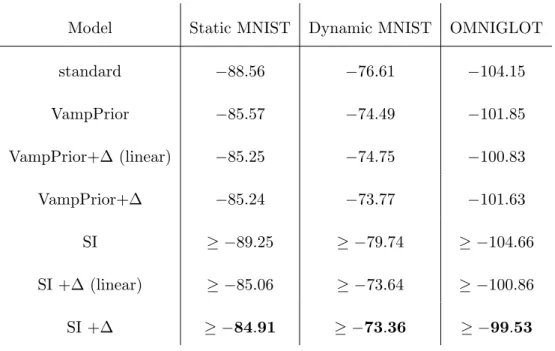
log ˆZk with Rao-Blackwellization

Exact Iteration 8 Iteration 6 Iteration 4 Iteration 2 Iteration 1 k 1 10 20 30 40 50 60 70 80 90 100 -12 -10 -8 -6 -4 -2 0

log ˆck with Rao-Blackwellization

logrk k 1 10 20 30 40 50 60 70 80 90 100 100 110 120 130 140 150 160 170 log ˆZk Exact Iteration 8 Iteration 6 Iteration 4 Iteration 2 Iteration 1 k 1 10 20 30 40 50 60 70 80 90 100 -12 -10 -8 -6 -4 -2 0 log ˆck logrk

Figure 2.1: Comparison of log ˆZk and log ˆck estimates, in some of the first eight iterations of the

initialization procedure described in Section 2.2.4, with and without Rao-Blackwellization, with K = 100. The initial values were ˆZk = 1 for all k, and the prior was uniform, rk = 1/K. The

model is a RBM with 784 visible and 10 hidden units, trained on the MNIST dataset. Each iteration consists of 50 Gibbs sweeps, on each of 100 parallel chains. Since in the non-Rao-Blackwellized case, the updates are unstable and sometimes infinite, for demonstration purposes only, we define ˆ

ck∝0.1 +PNi=1δk,k(i) and normalize. Note that in the Rao-Blackwellized case, the values of ˆck in

the final iteration are very close to those of rk, signaling that the ˆZk’s are good enough for a last,

Algorithm 2 Rao-Blackwellized Tempered Sampling Input: _{βk, rk}k=1,...,K, N Initialize log ˆZk, k= 2, ..., K Initialize β _{∈ {}β1, ..., βK} Initialize ˆck= 0, k= 1, ..., K for i= 1 toN do

Transition in xleaving q(x|β) invariant. Sampleβ_|x_∼(β_|x) Update ˆck←ˆck+_N1q(βk|x) end for Update ˆZRTS k ←Zˆk r1ˆck rkˆc1, k = 2, ..., K

Because β_k(i) was sampled from q(β|x(i)), we can reduce variance by Rao-Blackwellizing the first

sum in (2.13), resulting in LRB[Z] = N X i=1 K X k=2 log(Zk)q(βk|x(i)) −Nlog K X k=1 rkZk/Zˆk ! +const, =N K X k=2 log(Zk)ˆck (2.14) −Nlog K X k=1 rkZk/Zˆk ! +const .

The normalizing constants are estimated by maximizing (2.14) subject to a fixed Z1, which is

known. Setting the derivatives of (2.14) w.r.t. Zk’s to zero gives a system of linear equations

K X k0₌₂ rk0 ˆ Zk0 δk0_,k ˆ ck − 1 Zk0 =r₁ k= 2, . . . , K whose solution is (2.12).

2.2.4 Initial iterations

As mentioned above, the chain with initial ˆZk’s may mix slowly and provide a poor

estima-tor (i.e. small q(βk)’s are rarely sampled). Therefore, when the ˆZk’s are far from the Zk’s (or

equivalently, therk’s are far from the ˆck’s), the ˆZk’s estimates should be updated.

Our estimator in (2.12) does not directly handle the case where ˆZk is sequentially updated.

We note that the likelihood approach of (2.14) is straightforwardly adapted to this case and is

straightforwardly numerically optimized (see Section 2.4.4 for details). A simpler, less

computa-tionally intensive, and equally effective strategy is as follows: start with ˆZk= 1 for allk(or a better

estimate, if known), and iterate between estimating ˆck with few MCMC samples and updating ˆZk

with the estimated ˆZRTS

k using (2.12). In our experiments using many parallel Markov chains, this

procedure worked best when the updated Markov chains started from the previous last x’s, and

fresh, uniformly random sampled βk’s.

Once the ˆZk’s estimates are close enough to the Zk’s to facilitate mixing, a long MCMC chain

can be run to provide samples for the estimator. Because ˆck estimatesq(βk), andq(βk)'rk when

ˆ

Zk ' Zk, a simple stopping criterion for the initial iterations is to check the similarity between

ˆ

ck and rk. For example, if we use a uniform prior rk = 1/K, a practical rule is to iterate the

few-samples chains until maxk|rk−cˆk|<0.1/K.

Figure 2.1 shows the values taken by ˆZk and ˆck in these initial iterations in a simple example.

The figure also illustrates the importance of using the Rao-Blackwellized form (2.9) for ˆck, which

2.2.5 Bias and variance

Using (2.11)-(2.12) and log(1 +x)_'x₋x2_{/2, gives}

log ˆZ_kRTS≈logZk+ ∆ck qk − ∆c1 q1 − (∆ck)2 2q2 k +(∆c1) 2 2q2 1 (2.15)

whereqk=q(βk) and ∆ck= ˆck−qk. Taking expectations gives

E h log ˆZ_kRTSi₋logZk≈ 1 2 σ2 1 ˆ c2 1 − σ 2 k ˆ c2 k , (2.16) and Var[log ˆZRTS k ]≈ σ2 1 ˆ c2 1 +σ 2 k ˆ c2 k −2σ1k ˆ ckˆc1 (2.17) whereσ2

1 = Var[ˆc1], σ_k2 = Var[ˆck], andσ1k= Cov[ˆc1,cˆk].

This shows that the bias of log ˆZk has no definite sign. This is in contrast to many popular

methods, such as AIS, which underestimates logZk [Neal, 2001], and RAISE, which overestimates

logZk [Burda et al., 2015].

From the Central Limit Theorem, the asymptotic variance of ˆck is

V ar(ˆck) =

V arq(q(βk|x))ak

N , (2.18)

where the factor

ak= 1 + 2 ∞ X i=1 corrhq(βk|x(0)), q(βk|x(i)) i (2.19)

takes into account the autocorrelation of the Markov chain. But estimates of this sum from the

MCMC samples are generally too noisy to be useful. A more practical approach is to estimate

2.3

Related work

In this section, we briefly review some popular estimators and explore their relationship to

the proposed RTS estimator (2.12).

2.3.1 Wang-Landau

A well-known approach to obtain approximate values of the Zk’s is the Wang-Landau

algo-rithm [Wang and Landau, 2001; Atchade and Liu, 2010]. The setting is similar to ours, but the

algorithm constantly modifies the ˆZk’s along the Markov chain as differentβk’s are sampled. The

factors that change the ˆZk’s asymptotically converge to 1. The resulting ˆZk estimates are

usu-ally good enough to allow mixing in the (x, β) space [Salakhutdinov, 2010], but are too noisy for

purposes such as likelihood estimation [Tan, 2016].

2.3.2 AIS/RAISE

Annealed Importance Sampling (AIS) [Neal, 2001] is perhaps the most popular method in the

machine learning literature to estimate logZK. Here, one starts from a samplex1 fromp1(x), and

samples a point x2, using a transition function K2(x2|x1) that leaves f2(x) invariant. The process

is repeated until one has sampled xK using a transition function that leaves f(x) invariant. The

vector (x1, x2, ..., xK) is interpreted as a sample from an importance distribution on an extended

space, while the original distribution p(xK) can be similarly augmented into an extended space.

The resulting importance weight can be computed in terms of quotients of the fk’s, and provides

an unbiased estimator forZK/Z1, whose variance decreases linearly withK. Note that the inverse

temperatures in this approach are not random variables.

The variance of the AIS estimator can be reduced by averaging over several runs, but the

positive bias when estimating data log-likelihoods.

Recently, a related method, called Reverse Annealed Importance Sampling (RAISE) was

pro-posed to estimate the data log-likelihood in models with latent variables, giving negatively biased

estimates [Burda et al., 2015], [Z. et al., 2015]. The method performs a similar sampling as AIS,

but starts from a sample of the latent variables at βK = 1 and proceeds then to lower inverse

temperatures. In certain cases, such as in the RBM examples we consider in Section 2.4.2, one can

obtain from these estimates of the data log-likelihood an estimate of the partition function, which

will have a positive bias. The combination of the expectations of these AIS and RAISE estimators

thus ‘sandwiches’ the exact value [Burda et al., 2015], [Z. et al., 2015].

2.3.3 BAR/MBAR

Bennett’s acceptance ratio (BAR) [Bennett, 1976], also called bridge sampling [X.-L.Meng

and Wong, 1996], is based on the identity

Zk

Z1

= Ep(x|β1)[α(x)fk(x)]

Ep(x|βk)[α(x)f1(x)]

, (2.20)

where α(x) is an arbitrary function such that R f1(x)fk(x)α(x)dx < ∞, which can be chosen to

minimize the asymptotic variance. BAR has been generalized to estimate partition functions when

sampling among multiple distributions, a method termed the multistate BAR (MBAR) [Shirts and

Chodera, 2008].

Assuming that there are nk i.i.d. samples for each inverse temperature βk (N samples

be obtained by maximizing the log-likelihood function [Tan et al., 2012]: L[Z] = 1 N N X i=1 log K X k=1 nk N exp(−logZk+βk∆xi) ! + K X r=1 nr N logZr (2.21)

This method was recently rediscovered and shown to compare favorably against AIS/RAISE in [Liu

et al., 2015]. MBAR has many different names in different literatures, e.g. unbinned weighted

histogram analysis method (UWHAM) [Tan et al., 2012] and reverse logistic regression [Geyer,

1994].

Unlike RTS, MBAR does explicitly use q(β) when estimating the partition function. As a

price associated with this increased generality, MBAR requires the storage of all collected samples,

and the estimator is calculated by finding the maximum of (2.21). This likelihood function does

not have an analytic solution, and Newton-Raphson was proposed to iteratively solve this problem,

which requires _O(N K2 _+K3_{) per iteration. While RTS is less general than MBAR, RTS has an}

analytic solution and only requires the storage of the ˆck statistics. We note that this objective

function is very similar to the one discussed in Section 2.4.4 for pooling across samples collected

using different ˆZk’s.

Recent work has proposed a stochastic learning algorithm based on MBAR/UWHAM [Tan

et al., 2016]. This algorithm gives updates based on the sufficient statistics ˆck with

log ˆZ_k(t+1) = log ˆZ_k(t)+γt ˆ ck rk − ˆ c1 r1 . (2.22)

γt is a step size that is recommended to be set toγt=t−1. We note that our estimator from (2.12)

in log space may be written in a similar form, as logˆck

rk

−logcˆ1

r1

, which is very related in

form to (2.22). We empirically found that when the partition function estimates are far away from

estimator in (2.15) is the same as the term in (2.22), the updates will essentially only differ by the

selection of the step size γt when ˆck'rk.

2.3.4 Thermodynamic integration

Thermodynamic Integration [Gelman and Meng, 1998] is derived from basic calculus identities.

Let us first assume thatβis a continuous variable in [0,1]. We again define ∆x = logf(x)−logp1(x),

and fβ(x) =f(x)βp1(x)1−β. We note that

d dβlogZ(β) = Z ₁ Z(β) d dβfβ(x)dx =Ex|β[∆x], (2.23)

From calculus, we have

log ZK Z1 = Z 1 0 Ex|β[∆x]dβ =Ep(x|β)p(β) ∆x p(β)

This equation holds for anyp(β) that is positive over the range [0,1], and provides an unbiased

estimator for logZk if unbiased samples fromp(x|β) are available. This is in contrast to AIS, which

is unbiased onZk, and biased on logZk. Given samples{x(i), β(i)}i=1,...,N, the estimator for logZK

is \ logZK = logZ1+ 1 N N X i=1 ∆_x(_i) p(β(i)₎

There are two distinct approaches for generating samples and performing this calculation in

TI. First, β can be sampled from a prior p(β), and samples are generated fromfβ(x) to estimate

the gradient at the current point inβ space. A second approach is to use samples generated from

simulated tempering, which can facilitate mixing. However, the effective marginal distributionq(β)

must be estimated in this case.

When β consists of a discrete set of inverse temperatures, the integral can be approximated

integration, which can help in some cases [Friel et al., 2014]. As noted by [Calderhead and Girolami,

2009], this discretization error can be expressed as a sum of KL-divergences between neighboring

intermediate distributions. If the KL-divergences are known, an optimal discretization strategy can

be used. However, this is unknown in general.

While the point of this paper is not to improve the TI approach, we note that the

Rao-Blackwellization technique we propose also applies to TI when using tempered samples. This gives

that the Monte Carlo approximation of the gradient (2.23) is

d dβlogZ(β) β=βk ' N X i=1 q(βk|xi)∆xi PN j=1q(βk|xj) . (2.24)

This reduces the noise on the gradient estimates, and improves performance when the number

of bins is relatively high compared to the number of collected samples. We refer to this technique

as TI-Rao-Blackwell (TI-RB).

TI-RB is further interesting in the context of RTS, because of a surprising relationship: in

the continuous β limit, RTS and TI-RB areequivalent estimators. However, when using discrete inverse temperatures, RTS does not suffer from the discretization error that TI and TI-RB do.

2.4

Examples

In this section, we study the ability of RTS to estimate partition functions in a Gaussian

mixture model and in Restricted Boltzmann Machines and compare to estimates from popular

existing methods. We also study the dependence of several methods on the number K of inverse

temperatures, and show that RTS can provide estimates of train- and validation-set likelihoods

1000 1500 2000 2500 3000 3500 4000 −1 0 1 2 3 Number of samples log RMSE RTS MBAR TI Riemann TI trap TI trap corrected TI RB

Figure 2.2: Comparison of logZ estimation performance on a toy Gaussian Mixture Model using an RMSE from 10 repeats. TI Riemann approximates the discrete integral as a right Riemann sum, TI trap uses the trapezoidal method, TI trap corrected uses a variance correction technique, TI RB uses the Rao-Blackwellized version of TI.

2.4.1 Gaussian mixture example and comparisons

Figure 2.2 compares the performance of RTS to several methods, including MBAR and TI

and its variants, in a mixture of two 10-dimensional Gaussians (see Section A.2 for specific details).

The sampling was performed using a novel adaptive Hamiltonian Monte Carlo method for tempered

distributions of continuous variables, introduced in Section A.2. In this case the exact partition

function can be numerically estimated to high precision. Note that the estimators essentially give

identical performance; however, our method is the simplest to implement and use for tempered

samples, with minimal memory and computation requirements.

2.4.2 Partition functions of RBMs

The Restricted Boltzmann Machine (RBM) is a bipartite Markov Random Field model popular

in the machine learning community [Smolensky, 1986]. For the binary case, this is a generative

10

10

10

Gibbs Sweeps

450

451

452

453

454

E

st

im

at

or

M

ea

n

10

10

10

Gibbs Sweeps

0

0.5

1

1.5

2

2.5

E

st

im

at

or

R

M

S

E

10

10

10

10

Gibbs Sweeps

283

284

285

286

287

E

st

im

at

or

M

ea

n

10

10

10

10

Gibbs Sweeps

0

0.5

1

1.5

2

E

st

im

at

or

R

M

S

E

Figure 2.3: Mean and root mean squared error (RMSE) of competing estimators of logZKevaluated

on RBMs with 784 visible units trained on the MNIST dataset. The numbers of hidden units were 500 (Top) and 100 (Bottom). In both cases, the bias from RTS decreases quicker than that of AIS and RAISE, and the RMSE of AIS does not approach that of RTS at 1000 Gibbs sweeps until over an order of magnitude later. Each method is run on 100 parallel Gibbs chains, but the Gibbs sweeps in the horizontal axis corresponds to each individual chain.

vT_c+vT_{W h+h}T_{b, for parameters c∈}

RM,b∈RJ, andW ∈RM×J. A fundamental performance

measure of this model is the log-likelihood of a test set, which requires the estimation of the log

partition function. Both AIS [Salakhutdinov and Murray, 2008] and RAISE [Burda et al., 2015]

were proposed to address this issue. We will evaluate performance on the bias and the root mean

average of estimates from AIS and RTS with 106 _{samples from 100 parallel chains. We note the}

variance of these estimates was very low (≈0.006).

Figure 2.3 shows a comparison of RTS versus AIS/RAISE on two RBMs trained on the

bina-rized MNIST dataset (M=784, N=60000), with 500 and 100 hidden units. The former was taken

from [Salakhutdinov and Murray, 2008],1 _{while the latter was trained with the method of [Carlson}

et al., 2015].

In all the cases we used for p1 a product of Bernoulli distributions over thev variables which

matches the marginal statistics of the training dataset, following [Salakhutdinov and Murray, 2008].

We run each method (RTS, AIS, RAISE) with 100 parallel Gibbs chains. In RTS, the number

of inverse temperatures was fixed at K=100, and we performed 10 initial iterations of 50 Gibbs

sweeps each, following Section 2.2.4. In AIS/RAISE, the number of inverse temperatures K was set

to match in each case the total number of Gibbs sweeps in RTS, so the comparisons in Figure 2.3

correspond to matched computational costs. We note that the performance of RAISE is similar to

the plots shown in [Burda et al., 2015] for these parameters.

2.4.3 Number of temperatures

An advantage of the Rao-Blackwellization of temperature information is that there is no need

to pick a precise number of inverse temperatures, as long as K is big enough to allow for good

mixing of the Markov chain. As shown in Figure 2.4, RTS’s performance is not greatly affected by

adding more temperatures once there are enough temperatures to give good mixing.

Also note that as the number of temperatures increases RTS and the Rao-Blackwellized

ver-sion of TI (TI-RB) become increasingly similar. We show explicitly in Section A.4 that they are

equivalent in the infinite limit of the number of temperatures. Due to computational costs, running

1_{Code and parameters available from:}

101 102 103 Number of Temperatures 0.2 1 5 E st im a to r R M S E RTS TS MBAR TI TI-RB

Figure 2.4: RMSE as a function of the number of inverse temperatures K for various estimators. The model is the same RBM with 500 hidden units studied in Figure 2.3. Each point was obtained by averaging over 200 estimates (20 for MBAR due to computational costs) made from 10,000 bootstrapped samples from a long MCMC run of 3 million samples.

MBAR on a large number of temperatures is computationally prohibitive. An issue when estimates

are non-Rao-Blackwellized is that the estimates eventually become unstable as we do not have

positive counts for each bin. This is addressed heuristically in the non-Rao-Blackwellized version

of RTS (TS) by adding a constant of .1 to each bin. For TI, empty bins are imputed by linear

interpolation.

2.4.4 Tracking partition functions while training

There are many approaches to training RBMs, including recent methods that do not require

sampling [Sohl-Dickstein et al., 2010; Im et al., 2015; Gabrie et al., 2015]. However, most learning

algorithms are based on Monte Carlo Integration with persistent Contrastive Divergence [Tieleman

and Hinton, 2009]. This includes proposals based on tempered sampling [Salakhutdinov, 2009;

Desjardins et al., 2010]. In these cases, the slow speed of change of the parameters and the relatively

likelihoods during RBM training at minimal additional cost. This allows us to avoid overfitting by

early stopping of the training. We note that there are previous more involved efforts to track RBM

partition functions, which involve additional computational and implementation efforts [Desjardins

et al., 2011].

This idea is illustrated in Figure 2.5, which shows estimates of the mean of training and

validation log-likelihoods on the dna dataset2_{, with 180 observed binary features, trained on a}

RBM with 500 hidden units.

We first pretrain the RBM with CD-1 to get initial values for the RBM parameters. We

then run initial RTS iterations with K = 100, as in Section 2.2.4, in order to get starting log ˆZk

estimates.

For the main training effort we used the RMSspectral gradient method, with stepsize of 1e-5

and parameterλ=.99 (see [Carlson et al., 2015] for details). We considered a tempered space with

K = 100 and sampled 25 Gibbs sweeps on 2000 parallel chains between gradient updates. The

latter is a large number compared to older learning approaches [Salakhutdinov and Murray, 2008],

but is similar to that used both in [Carlson et al., 2015] and [Grosse and Salakhudinov, 2015] that

provide state-of-the-art learning techniques.

With the samples collected after each 25 Gibbs sweeps, we can estimate the ˆck’s to compute

the running partition function. To smooth the noise from such a small number of samples, we

consider partial updates of ˆZK given by

ˆ Z_K(t+1)= ˆZ_K(t) r1 rK ˆ c(_Kt) ˆ c(₁t) !α (2.25)

withα= 0.2, andtan index on the gradient update. Similar results were obtained with.05< α <

.5. This smoothing is also justified by the slowly changing nature of the parameters. Figure 2.5 also

2_{Available from:}

0

2000

4000

6000

8000

Iteration

-100

-90

-80

-70

-60

-50

h

lo

g

p

(

v

)

i

Figure 2.5: A demonstration of the ability to track with minimal cost the mean train and validation log-likelihood during the training of a RBM on thedna 180-dimensional binary dataset, with 500 latent features.

shows the corresponding value from AIS with 100 parallel samples and 10,000 inverse temperatures.

Such AIS runs have been shown to give accurate estimates of the partition function for RBMs with

even more hidden units [Salakhutdinov and Murray, 2008], but involve a major computational cost

that our method avoids. Using the settings from [Salakhutdinov and Murray, 2008] adds a cost of

106 _{additional samples.}

2.5

Discussion

In this paper, we have developed a new partition function estimation method that we called

Rao-Blackwellized Tempered Sampling (RTS). Our experiments show RTS has equal or superior

performance to existing methods popular in the machine learning and physical chemistry

commu-nities, while only requiring sufficient statistics collected during simulated tempering.

An important free parameter is the prior over inverse temperatures,rk, and its optimal

selec-tion is a natural quesselec-tion. We explored several parametrized proposals forrk, but in our experiments

continuous β formulation, but the resulting estimates were less accurate. Additionally, we tried

subtracting off estimates of the bias, but this did not improve the results. Finally, we tried

incor-porating a variety of control variates, such as those in [Dellaportas and Kontoyiannis, 2012], but

did not find them to reduce the variance of our estimates in the examples we considered. Other

control variates methods, such as those in [Oates et al., 2015], could potentially be combined with

Chapter 3

Decoupling aggregate priors in

variational autoencoders

The choice of the generative model prior is an important part of designing variational

au-toencoders. The variational posterior averaged over the data distribution uniquely minimizes the

evidence lower bound (ELBO) with respect to the prior; consequently, a popular prior choice is a

direct estimate of the variational posterior by averaging a fixed number of encoding distributions.

However, since the encoding model is regularized by the prior in the ELBO, such direct coupling

of the prior and variational distribution leads to additional constraints on the encoding model,

which can limit performance. We propose a generalization of the aggregate approximation prior by

endowing it with generic ‘delta’ functions parameterized independently from the encoder, giving

rise to a more flexible prior capable of decoupling from the encoder model, which we show improves

the latent representation. We also show that when this approach is used in conjunction with a

semi-implicit aggregate prior, it greatly improves performance and gives superior log-likelihoods

compared to existing aggregate models. Finally, we draw a parallel between the decoupled

3.1

Introduction

Generative modeling, which aims to learn and produce samples from a dataset’s underlying

probability distribution, is a major goal of machine learning. Variational autoencoders (VAEs) [Kingma and Welling, 2014; D.J. Rezende, 2014] have become very popular over the past few

years partly due to their combining inference and generative modeling into one framework, with

the evidence lower bound (ELBO) on the marginal log-likelihood reflecting both the inference and

generative models. Integral to its success is the reparameterization trick, which enables stochastic

gradients of the ELBO to leverage the latent space density’s parametric form, thereby reducing

variance.

A common consequence of the latent distribution’s parametric form is that it can be overly

simplistic relative to the true posterior and cannot accurately approximate it, represented by the

gap between the ELBO and the marginal log-likelihood. Consequently, efforts have been made to

increase the variational distribution’s expressiveness including using flow-based models [Rezende

and Mohamed, 2015; Kingma et al., 2016; van den Berg et al., 2018; Chen et al., 2018], implicit

variational models [Huszar, 2017; Mescheder et al., 2017; Tran et al., 2017; Yin and Zhou, 2018;

Shi et al., 2018], adversarial models [Mescheder et al., 2017], and Bayesian nonparametric models [Tran et al., 2016; Nalisnick and Smyth, 2017]

However, due to being regularized by the generative model’s prior, the variational distribution

may not reach its full expressive capacity even under more sophisticated encoder models. Due to

the nature of the KL-divergence penalty, the variational distribution will tend to avoid putting

probability density in regions in which the prior’s density is low [Ranganath et al., 2016],

poten-tially limiting the variational model. Another drawback of overregularization of the variational

vari-able is drawn from the prior’s wider density [Makhzani et al., 2016]. When the decoder model is

sophisticated enough, for example in autoregressive decoders (e.g., [van den Oord et al., 2016a;

van den Oord et al., 2016b], the KL penalty may prevent the model from learning a useful

encoding entirely [Alemi et al., 2017], and optimization heuristics must be used, including

an-nealing the KL penalty at the start of training [Bowman et al., 2016; Sønderby et al., 2016;

Serban et al., 2017] or effectively eliminating the KL penalty up to some quantity [Kingma et al.,

2016]. Additionally, specific modeling constraints can be put on the decoder to require the latent

space to be informative [Chen et al., 2017].

Designing the prior has received less attention than the variational distribution, perhaps due

to its perceived relative simplicity, or that many of the methods used to increase the expressivity of

the encoding model (e.g., flow-based and autoregressive models) can be used similarly for the prior.

In this paper, we restrict our attention to models that use for the prior an approximation of the

ag-gregate variational posterior that is either explicit [Tomczak and Welling, 2018] or (semi-) implicit

[Molchanov et al., 2019]. An alternate expression of the ELBO by [Hoffman and Johnson, 2016]

using a marginal KL penalty served as motivation for these models, as the penalty is minimized

by the aggregate variational distribution. However, we argue that alone, these approximations can

place unnecessary constraints on the encoder model and hinder overall performance. Thus, the

aggregate approximation prior still has an effect on the encoding model, despite the technique’s

motivation to simply minimize one term in the ELBO. In fact, as we show empirically, a better

prior can even increase the marginal KL if the reconstruction quality is sufficiently improved.

We propose a generic decoupling model to endow the prior with flexibility while still utilizing

information about the encoder, which we show improves reconstruction and latent representation

quality. Decoupling the semi-implicit prior in particular leads to superior test log-likelihoods over

approxima-tion. Finally, we draw a connection between the decoupled semi-implicit model and kernel density

estimation.

3.2

Variational Autoencoders

Given some data,{xn}Nn=1, xn ∼ptrue(x), latent variable models circumvent direct modeling

of the observed data and instead assume a set of stochastic unobserved variables z interact

ac-cording to p(z) and influence the observed variables according to p(x|z). However, the posterior probability p(z_|x) is often intractable to compute. Instead, variational inference [Jordan et al., 1999] introduces a variational distributionq(z) that functions as a tractable approximation to the

posterior distribution.

Without access top(z_|x), variational inference aims to maximize not the marginal log-probability logp(x) but rather an expected lower bound on it (the ELBO):

L(x),Eq(z|x)[logp(x, z)−logq(z|x)], (3.1)

where we have amortized the variational distribution by making it a function ofx. The variational

autoencoder [Kingma and Welling, 2014; D.J. Rezende, 2014] uses two separate deterministic

feed-forward neural networks to modelq(z_|x) andp(x_|z), called the recognition (or encoder) model and the generative model, respectively. Specification of the prior p(z) completes the model.

In contrast to undirected generative models [Dayan et al., 1995; Hinton and Salakhutdinov,

2006], sampling from the latent space requires only one feedforward ‘sweep.’ Additionally, as

op-posed to stochastic neural networks [Neal, 1992; Mnih and Gregor, 2014; Mnih and Rezende, 2016]

the simple parametric form ofq(z_|x) enables the use of the ‘reparameterization trick’ [Kingma and Welling, 2014; D.J. Rezende, 2014], which expresses latent samples as functions of parameters of

The ELBO can be rewritten as

L(x) =Eq(z|x)[logp(x, z)−logq(z|x)]

=Eq(z|x)[logp(x|z)]−DKL(q(z|x)||p(z)), (3.2)

where we can interpret the first term as encouraging the recognition model to provide latent samples

to generative model which will give rise to reconstructions that match the data, while the second

term functions as a complexity penalty.

3.3

Prior Choice

Until recently, the prior has received little attention, potentially because from a modeling

perspective, a sufficiently complex decoderp(x_|z) should be able to transform a base distribution such as the standard Gaussian into a potentially highly complicated marginal distribution over the

observed space (see e.g., [Goodfellow et al., 2014]). However, from Equation (3.2), we see that the

ELBO is regularized by the encoding distribution’s deviation from the prior, so even if a basic prior

can produce good samples with the right generative model, if the encoder cannot find a good latent

representation, the model will be poor.

3.3.1 Aggregate priors

A key observation by [Hoffman and Johnson, 2016] was that the ELBO averaged over the

training set{xn}Nn=1 can be rewritten as

L(θ, φ) = 1 N N X n=1 Eq(z|xn)[logp(xn|z)]−(logN −Eq(z)[H[q(n|z)]])−KL(q(z)||p(z)) (3.3) = 1 N N X n=1 Eq(z|xn)[logp(xn|z)]−MI[n, z]−KL(q(z)||p(z)), (3.4) whereH[·] is entropy,q(n|x) = q(z|xn)_qp_(zdata₎ (xn) = PNq(z|xn)

i=1q(z|xi),and MI[·,·] is mutual information. We see from Equation (3.4) that the ELBO consists of a data-dependent reconstruction term