Nested VAE:Isolating Common Factors via Weak Supervision

NestedVAE: Isolating Common Factors via Weak Supervision.

Matthew J. Vowels

Necati Cihan Camgoz

Richard Bowden

Centre for Vision, Speech and Signal Processing

University of Surrey

Guildford, UK

Abstract

Fair and unbiased machine learning is an important and active field of research, as decision processes are increas-ingly driven by models that learn from data. Unfortunately, any biases present in the data may be learned by the model, thereby inappropriately transferring that bias into the de-cision making process. We identify the connection between the task of bias reduction and that of isolating factors com-mon between domains whilst encouraging domain specific invariance. To isolate the common factors we combine the theory of deep latent variable models with information bot-tleneck theory for scenarios whereby data may be naturally paired across domains and no additional supervision is re-quired. The result is the Nested Variational AutoEncoder (NestedVAE). Two outer VAEs with shared weights attempt to reconstruct the input and infer a latent space, whilst a nested VAE attempts to reconstruct the latent representation of one image, from the latent representation of its paired im-age. In so doing, the nested VAE isolates the common latent factors/causes and becomes invariant to unwanted factors that are not shared between paired images. We also pro-pose a new metric to provide a balanced method of evaluat-ing consistency and classifier performance across domains which we refer to as the Adjusted Parity metric. An evalua-tion of NestedVAE on both domain and attribute invariance, change detection, and learning common factors for the pre-diction of biological sex demonstrates that NestedVAE sig-nificantly outperforms alternative methods.

1. Introduction

One of the goals of representation learning is to achieve an embedding that informatively captures the underlying factors of variation in data [10]. However, many techniques for learning such embeddings have been found to also learn unwanted or confounding factors, irrelevant or detrimental to the intended task(s) [54]. Such factors can include dis-tribution specific bias, which impairs the generalizability of a model across empirical samples or in the face of

distri-z

z

z

x

x

ˆ

x

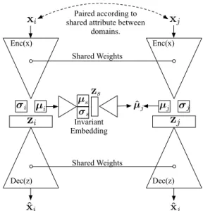
domains. Shared Weights Shared Weights Enc(x) Enc(x) Dec(z) Dec(z) Invariant Embedding ˆ µj µj σj σi µi _σ s µs

Figure 1. Top-level architecture of NestedVAE. Images (or alter-native data modality) are paired according to shared attributes or domains. Latent representationsziandzjfor imagesxiandxj are derived and fed to a secondary ‘nested’ VAE. Using the princi-ples from Information Bottleneck theory, a sufficient and minimal representationzs forzjmay be derived fromziand vice versa.

zsmay therefore be interpreted as representing the common fac-tors, or common causes for the two images. Sufficiency indicates it contains the information common to both, and minimality indi-cates that it is invariant to information specific to each.

butional shift [14, 54, 74, 11], or bias associated with cul-turally sensitive or legally protected characteristics such as race, age, gender or sex [55, 17, 53, 36, 71, 57, 65, 15].

Indeed, the prevalence of reports of systemic bias aris-ing from the use of machine learnaris-ing algorithms is increas-ing [35, 66, 77]. Furthermore, conceptually distinct factors, such as object type and pose, may be entangled in the em-bedding, despite a prior expectation that they ought to be factorized. Learning models that solve these problems is therefore important from a number of converging ing and societal perspectives [55]. In terms of

engineer-xi xj zs

z

z

θ

φ

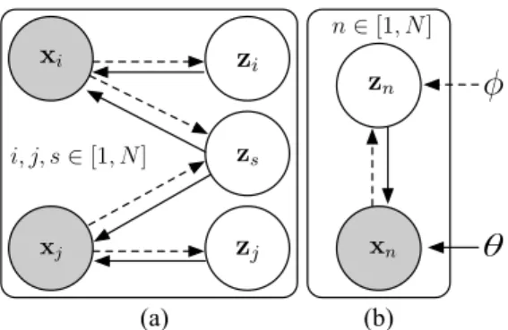
Figure 2. Probabilistic Graphic Model for (a) inferring the com-mon factors zs from pairs of imagesxi andxj and (b) the in-ference and generative processes of a VAE. Dotted lines indicate inference and solid lines indicate generation.φandθare the VAE encoder (inference) and decoder (generation) parameters respec-tively.

ing, we may wish for our models to be informative, to be invariant to nuisance factors, to perform well and gener-alize across domains, and to disentangle independent fac-tors of variation. From a societal perspective, we may wish to achieve statistical and demographic parity such that our models do not reflect or amplify any unfairness present in our data or in society itself [65, 91, 35, 66].

Success at these overlapping tasks has implications for a range of more specific downstream tasks including attribute transfer [80, 81, 33, 39, 94], person re-identification [8, 27], change detection [32] adversarial robustness [37], and ma-chine learning based decision processes [55, 9, 63].

The contributions of this work are as follows:

• A unified interpretation of prior work on bias, disen-tanglement, fairness, domain/attribute invariance, and common causes.

• A novel deep latent variable model (Figure 1) called the Nested Variational Autoencoder (NestedVAE) that combines deep, amortized variational inference [43] and Information Bottleneck (IB) theory [82, 83].

• A demonstration that NestedVAE achieves significant improvements in classification and regression by learn-ing the common factors between domains.

• A novel metric for evaluating regression and classifica-tion parity across domains, referred to as the Adjusted Parity Metric, that accounts for predictive performance and the variation in performance across domains.

2. Formulation

2.1. Problem Formulation

We consider the problem of encoding an informa-tive, latent representation z _∼ p(z) from observation

x _∼ p(x_|z,c) such that z is invariant to some irrele-vant/nuisance/confounding covariatec[58]. From a statis-tical parity perspective, we wish to be able to use the latent

representation for some arbitrary downstream prediction of labelysuch thatp(ˆy =y_|c,z) =p(ˆy=y_|z)_∀y,c,z[56]. We therefore wish forz_⊥⊥candy _⊥⊥c. From a domain invariance perspective, we wish learning to transfer as much as possible between the different domains, where each do-main is associated with its own confounders or covariates. In other words, the learnt latent representation should be in-dependent of nuisance or confounding factors, thereby re-sulting in downstream task performance that is invariant to these factors. Further, the resulting representation will rep-resent the latent factors common to each domain.

For the development of NestedVAE, we consider the in-corporation of weak supervision whereby the supervision takes the form of data pairs [75]. Scenarios for which nat-ural pairings occur or may be straightforwardly derived in-clude: time series data whereby individuals appearing in frames from the same scene vary in terms of pose and ex-pression but maintain identity [23, 26]; pairings within do-mains where the dodo-mains may be hospitals or patients and the data may be medical images [54]; pairings arising from dyadic interactions such as conversations [40]; and pair-ings of data representing images of objects (e.g. hands from sign language data) from multiple viewpoints. With-out loss of generality we primarily consider the application of computer vision with face images, whereby the images are paired according to sex.

For the following formalization we assume two domains, although the model can be extended to include any number of domains for which we can form pairs. The Probabilis-tic Graphic Model (PGM) corresponding with our world model is depicted in Figure 2a. We assume that each im-agexi ∈X1andxj ∈X2has latent factors/causesziand zj specific to the respective domainsX1orX2, as well as

shared factors/causeszs common to both domains. From

the perspective of learning domain invariance, zi and zj

represent confoundersci andcj respectively, and X1 and

X2 represent different domains to which the

representa-tionzsshould be agnostic/invariant. From the perspectives

of causal modelling, zi andzj are domain specific latent

causes, andzsare common latent causes [50]. This is

simi-lar to the confounding additive noise model [38, 50] where

xi =fi(zi) +gi(zs) +iandxj =fj(zj) +gj(zs) +j,

f andgare arbitrary functions, andis additive noise. For each pair of images we wish to learn a representa-tion zs that represents only the common factors between

images in the pair. In order to do so, we leverage the infor-mation gain achieved from specific pairings in order to infer

zsfromziandzj, and take inspiration from the information

bottleneck perspective [82, 83, 65, 2]. To do so, we model the shared and common factors as a Markov chain:

zi−→zs−→zjs.t.p(zj|zi,zs) =p(zj|zs) (1)

The Data Processing Inequality [20] means thatzs

information about zj inzs can therefore only be what is

common to bothziandzj. The image pairings are formed

as non-ordered combinations such that we pairxi withxj

but alsoxjwithxi. As such, our task becomes that of

pre-dictingzj fromzi viazs. Finally, if we make the (albeit

strong) assumption thatzi≈zj+, whererepresents

ran-dom perturbations specific to the respective ran-domain, then we can apply VAEs to the task of learning the minimal and sufficient representationzsby seeking to generatezifrom zj, and vice versa. Sufficiency describes the Markov chain

condition in Eq. 1 wherebyI(zs;zj) =I(zi;zj), and

min-imality describes the fact that there is minimal redundant information in the representation [2, 20].1 _{In other words,} zsonly contains the information inzjwhich is also inzi.

2.2. VAEs

We now turn our attention to VAEs. For a detailed review of the theory, interested readers are directed to [24, 43, 70]. The PGM for the inference and generation (or, equivalently, encoding and decoding) processes of the VAE is shown in Figure 2b. Following the theory for variational inference [12] for a distribution of latent variablesz, we start by sam-plingz_∼p(z)and generate datasetX of imagesx_∈RN

with reconstructed/generated distributionpθ(x|z). We may

derive an inferred posterior for the conditional latent distri-bution asqφ(z|x)that approximates the true conditional

in-ference distributionpθ(z|x). Bothqφ(z|x)andpθ(x|z)are

parameterised by neural network encoder and decoder pa-rametersφandθrespectively [85, 24, 93]. The approximat-ing distributionqis chosen to circumvent the intractability of the integral when computing (in order to maximize) the marginal likelihoodp(x) = R pθ(x|z)p(z)dzand is

intro-duced according to the identity trick: logp(x) = log Z pθ(x|z) p(z) qφ(z|x) qφ(z|x)dz (2)

This may be further manipulated to establish a lower bound on the marginal log likelihoodlogp(x):

logpθ(x) =

Ez∼qφ(z|x)[logpθ(x|z)]−KL [qφ(z|x)||p(z)] +... ...+ KL [qφ(z|x)||pθ(z|x)]

(3)

The last term on the right hand side of Eq. 3 represents the divergence between our true inference distribution and our choice of approximating distribution, and forms what is known as the ‘approximation gap’ between the true log likelihood, and its estimation [61]. Once we choose our ap-proximating distribution and optimise it, we are unable to reduce this divergence further. This term is usually omitted such that we are left with what is known as either the Vari-ational Lower Bound (VLB) or the Evidence Lower Bound

1_{Here,I(.;.)is the Shannon mutual information.}

(ELBO), which serves as a proxy for the log-likelihood. We can then maximize the ELBO as follows [43, 47]:

max θ,φ Ex[LELBO(x)] = max θ,φ Ex Ez∼qφ(z|x)[logpθ(x|z)]−βKL (qφ(z|x)kp(z)) (4) The first term on the RHS of Eq. 4 encourages re-construction accuracy, and the Kullback-Liebler divergence term (weighted by parameterβ [33]) acts as a prior regu-larizer, penalising approximations forqφ(z|x) that do not

resemble the prior. The objective is therefore to maximise the lower bound to the marginal log-likelihood ofxover the latent distributionz[33], which is assumed to be Gaussian with identity covariancez_{∼ N}(0,I). If sample quality is not of primary concern, there is some incentive to weaken the decoder capacity in order to maintain pressure to encode useful information in the latent space (i.e. increaseI(x;z)) and to prevent decoupling of the decoder from the encoder [59]. The assumption of Gaussianity means that Eq. 4 may be written using an analytical reduction of the KL diver-gence term [47]: max θ,φ Ex[LELBO(x)] = maxθ,φ Ex Ez∼qφ(z|x)[logpθ(x|z)]− β 2 X i [Σφ(x)]ii−ln [Σφ(x)]ii +µ_φ(x) 2 2 (5) In Eq. 5 the [Σφ(x)]_ii indicates the diagonal

covari-ance, and µφ(x)is the mean. Both the mean and

covari-ance are learned by the network encoder and parameter-ize a multivariate Gaussian that forms the inferred latent distribution qφ(z|x). The decoder network samples from z _∼ qφ(z|x)using the reparameterization trick [24] such

thatz=µφ(x)+

p

Σφ(x)where we redefine=N(0,I).

One interpretation of disentanglement posits it is achieved ifqφ(z) =

R

qφ(z|x)p(x)dx=Qiqi(zi)[47].

Applying VAEs to our task: we can learn the latent fac-tors zi andzj for imagesxi ∼ X1 andxj ∼ X2

respec-tively. The following section describes the means to utilise these embeddings to learn the shared factorszs.

2.3. Combining VAEs and Information Bottleneck

L(p(z_|x)) =H(y_|z) +βI(z;x) (6) Notice thatH, the Shannon entropy of the conditional distribution, is equivalent to the cross-entropy reconstruc-tion term in Eq. 4, except that in VAEs the targetyisxand

the network generates a reconstruction xˆ _∼ p(ˆx_|z). Fur-ther, notice thatI(z;x) = ExKL [qφ(z|x)||p(z)]which is

the prior regularizer in Eq. 4. Finally theβterm is proposed to be learned via Lagrangian optimization [2] although, for VAEs, it may also be annealed during training [16] or eval-uated as a hyperparameter [33].

Making the assumption thatzi ≈zj+, we can

reap-ply the VAE model to this problem. As such, we apreap-ply an ‘outer’ VAE to the problem of learningzi andzj and

a ‘nested’ VAE to the problem of learning the common fac-torszs. The full loss function overxi ∼X1andxj ∼X2

is simply a combination of the outer and nested VAE ob-jectives for each image in a pair, and is presented in Eq. 7. Here,φ1,θ1, andφ2,θ2 are the encoder and decoder

pa-rameters for the ‘outer’ and ‘nested’ VAEs respectively. We have assumed the same prior distributionp(z)and the same approximating distribution familyqfor both outer and nested VAEs. max θ1,φ1,θ2,φ2 Exi∼X1,xj∼X2[LNested] = max θ1,φ1,θ2,φ2 Exij∼X1,X2[γ(L(xi,zi) +L(xj,zj)) +... ... λ(_L(zi,zs) +L(zj,zs))] (7) Here,γandλare hyperparameters that weight the outer and nested VAE ELBO functions respectively. Note that we optimise over all parametersφ1,θ1,φ2andθ2 jointly. In

summary, we propose to use VAEs to simultaneously learn both the latent factorszi for image xi and the latent

fac-torszj for imagexj, while ensuring a sufficient and

min-imal representationzs exists between these latent factors.

The network architecture is depicted in Figure 1. Note that, in practice, we find that feeding the nested VAE the latent codesµi andµj rather thanziandzj occasionally yields

better performance. Furthermore, we also find that theβ KL weight for the nested VAE should be set close to, or equal to zero for the best results. This is coherent with the application of IB to the derivation of common factors and therefore does not contradict the formulation: zsis being

derived from the commonality between the parametersµi

andµjof the latent random variablesziandzj, which have

already been regularized by the outer VAE. We can there-fore adjust the IB aspect of NestedVAE in Eq. 1 to:

µi q(z|µi)

−−−−→zs

p(µj|z)

−−−−→µj (8)

3. Prior Work: A Unifying Perspective

Previous work has aimed to achieve a range of seem-ingly distinct goals which include disentanglement, do-main/attribute invariance, fair encodings and bias reduction, generalization, and common causes. In this section, we re-view examples of such work, whilst drawing attention to the significant commonality between the goals. By noting the commonality, we hope that progress in one area may be leveraged to make progress in the others.

We have identified the problem of achieving domain in-variance, which is to transfer learning between domains whilst being invariant to the confounders and covariates unique to each domain. When such confounders are con-sidered to be ‘sensitive’ attributes, achieving domain invari-ance may also be considered to be achieving bias reduction, fairness, or demographic parity; when such confounders cause distributional shift, achieving invariance may be con-sidered to be achieving model generalization. Such tasks either require that the confounding information is ‘forgot-ten’ or ignored, or that it be disentangled from the domain invariant (i.e. task relevant) factors. However, the task of forgetting is often treated as being distinct from disentan-glement. We argue that these tasks complement each other: one researcher’s disentangled, generative attribute may be another’s confounder. For instance, in facial recognition, the identity of an individual should be predicted from an image in such a way that the prediction is invariant to the head-pose and facial expression; it does not benefit the model to provide a different identity representation for a different head-pose. For such an application, a method may either ‘learn to forget’ pose, or to disentangle head-pose from identity such that the information encoding iden-tity is independent of, and separable from, the information for pose. In both disentanglement and domain invariance, relevant information needs to be separated from task-irrelevant information.

Furthermore, many of the models utilised for disentan-glement are deep latent variable models [33, 46, 16, 26, 93, 47, 56]. Such models aim to infer the generative or causal factors behind the observed data. As such, us-ing these models to identify factors which are common between domains (as NestedVAE does) becomes equiva-lent both to identifying the common causes as well as to identifying the factors which generalize across domains. Much of the prior work on unsupervised disentanglement [33, 73, 75, 26, 16, 93, 47, 56] therefore also indirectly con-tributes to the field of domain invariance and fairness. In-deed, recent work [55] has specifically explored the connec-tion between disentanglement and fairness.

Previous research has sought to disentangle and/or learn invariant representations by incorporating supervision with fully supervised VAEs [46, 21], semi-supervised VAEs [57, 65, 54, 76], adversarial training [30, 31, 27, 74, 90, 88, 48, 60, 69, 94, 3], Shannon Mutual Information regular-ization [44, 68] and paired images with auxiliary classifiers [14, 8]. In other scenarios, we may only have access to indi-rect supervision force.g. in the form of grouped or paired images [81, 25, 1] or pairwise similarities [19, 18]. In such cases, previous work has incorporated such weak supervi-sion into VAEs [72, 23, 13, 19, 87], cycle-consistent net-works [39, 51], autoencoders [25], and autoencoders with adversarial training [80]. In scenarios whereby no

supervi-sion is available to assist in learning invariant embeddings, unsupervised approaches are possible which may involve testing for disentanglement and interventional robustness [79, 56]. Existing methods that aim to achieve domain in-variance and/or disentanglement therefore vary in the level of incorporation of supervision.

Acquiring high quality labelled datasets is both time con-suming and expensive, and supervised methods such as those that require labels for class, domain, and/or covariate (e.g. as for [3, 54]) may not always be feasibile. Disentan-glement may allow for an embedding to be learned such that the undesired covariate is identifiable or extricable at a later time for a specific downstream task. However, the efficacy of completely unsupervised methods for disentanglement has recently been shown to vary as much by random-seed as by architecture and design [56].

Given the disadvantages of both fully supervised and fully unsupervised methods, it is pertinent to consider meth-ods that incorporate minimal levels of weak supervision. Despite some overlap between definitions [29], weak super-vision is generally used to describe the scenario whereby labels are available but the labels only relate to a limited number of factors [80]. Semi-supervision, in contrast, de-scribes the scenario whereby fully informative labelling is available but only for a subset of the data [42]. Whilst ad-versarial methods have been shown to work well for ‘for-getting’ information, they are also notoriously difficult and unreliable to train [65, 52, 26]. Further, previous work has highlighted that adversarial training is unnecessary, and that non-adversarial training can achieve comparable or better results [65, 26]. Given the disadvantages of adversarial training and the comparable success of VAEs, we consider developing a new method using the VAE as a foundation. VAEs are a form of latent variable model [43] and are there-fore suitable for the task of deriving invariant representa-tions from observarepresenta-tions with limited supervision.

The closest prior work to ours in terms of architectural similarity is probably Joint Autoencoders for Disentangle-ment (JADE) [8]. JADE pairs images according to a com-mon label, feeds each image through a separate VAE and uses a partition from each VAE latent space to predict the shared label, thereby attempting to disentangle label rele-vant information from label irrelerele-vant information. JADE is evaluated according to its capacity for transfer learning from one, data abundant domain (the full MNIST dataset [49]) to a data scarce domain (chosen to be a reduced ver-sion SVHN dataset [67]). The NestedVAE differs in that we do not use labels indicating the domain, thereby signif-icantly weakening the level of explicit supervision. Work by [23] pairs images according to whether or not they de-rive from the same video sequence, and is classified by the researchers as being an unsupervised method. We take a similar approach with NestedVAE by pairing images, but

broaden the input pairings beyond those from the same video sequence to those that are from two domains but that share some common attribute(s). The result is a net-work that ‘forgets’ information specific to each domain, and learns factors common to both without adversarial training, and with only minimal, weak supervision.

4. Evaluation of NestedVAE

In light of the overlap between domain/attribute invari-ance, fairness, and bias reduction discussed in the previ-ous section, we evaluate NestedVAE on a range of tasks. NestedVAE is first evaluated for domain/attribute invariance and change detection on a synthetic dataset with ground-truth factors: rotated MNIST [28, 49]. For this first evalu-ation, NestedVAE is compared againstβ-VAE [33] (which increases the pressure on the KL-divergence loss), infoVAE [93] (which minimises maximum mean discrepancy) and DIP-VAE-I and DIP-VAE-II [47]. For a non-synthetic eval-uation, we test for fairness and bias reduction with biologi-cal sex prediction across individuals of different race using the UTKFace dataset [92], and compare with β-VAE and DIP-VAE-I. Additional results can be found in the supple-mentary material.

4.1. Adjusted Parity Metric

For evaluation of domain invariance we propose a (to the best of our knowledge) new parity metric that accounts for both discrepancies in accuracy between domains as well as classifier accuracy or normalized regressor performance. The metric is referred to in this work as the adjusted parity metric (adjusted for accuracy) and is defined as follows:

∆_adj= ¯S(1₋2σacc) (9) Here, S¯ is the average accuracy2 _{of the classifier over}

the domains, normalized to be between [0,1] according to the baseline accuracy of a random prediction. For exam-ple, if we have equal chance of predicting any of the 10 MNIST digits by random chance, the baseline is 0.1. σacc is the standard deviation of the normalized classifier accu-racies. Any classifier that is minimally consistentor mini-mally accurate will have∆_adj = 0and any classifier that is maximally consistentand maximally accurate will have ∆_adj = 1. This metric was motivated by the fact that al-though a representation may be domain or attribute invari-ant, this does not imply that it is also a good classifier: it must also be informative for the intended task.

4.2. Models

For the purposes of the evaluations in this work, the VAEs that constitute NestedVAE do not deviate from the 2_{Alternatively, the F1 score may be used, which is already normalized}

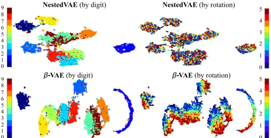
NestedVAE (by digit) NestedVAE (by rotation) 0 1 2 3 4 5 6 7 8 9 0 1 2 3 4 5

β-VAE (by digit) β-VAE (by rotation)

0 1 2 3 4 5 0 1 2 3 4 5 6 7 8 9

Figure 3. UMAP projections of the representations learned from the rotated MNIST dataset by NestedVAE andβVAE. The representations are coloured according to digit class (left) and rotation domain (right). It can be seen that NestedVAE representations contain significantly less information about rotation than do theβVAE representations. Best viewed in color.

Transfer Domain Nested (ours) β-VAE infoVAE DIP-VAE-I DIP-VAE-II

Digit Classification 0◦ 0.708±0.211 0.551±0.262 0.629±0.141 0.561±0.213 0.519±0.274 (higher is better) 15◦ 0.696±0.202 0.546±0.261 0.633±0.132 0.597±0.189 0.527±0.270 30◦ 0.714±0.152 0.555±0.251 0.657±0.076 0.602±0.206 0.539±0.244 45◦ 0.738±0.124 0.575±0.212 0.681±0.056 0.587±0.208 0.510±0.275 60◦ 0.721±0.127 0.573±0.203 0.682±0.057 0.577±0.224 0.487±0.278 75◦ 0.647±0.250 0.509±0.249 0.588±0.183 0.417±0.203 0.488±0.253 ¯

∆_{adj Parity} n/a 0.664 0.525 0.603 0.486 0.492 Rotation Classification 0◦ 0.373±0.029 0.530±0.011 0.523±0.005 0.511±0.012 0.541±0.007 (lower is better) 15◦ 0.343±0.008 0.534±0.005 0.516±0.008 0.493±0.007 0.547±0.005 30◦ 0.295±0.050 0.534±0.007 0.546±0.005 0.494±0.005 0.538±0.006 45◦ 0.316±0.025 0.532±0.006 0.540±0.001 0.493±0.007 0.541±0.003 60◦ 0.321±0.014 0.534±0.005 0.542±0.006 0.495±0.007 0.549±0.007 75◦ 0.347±0.057 0.517±0.012 0.509±0.010 0.496±0.016 0.518±0.012

Table 1. Average F1-scores and standard errors over 10 runs for digit class (higher is better) and rotation domain (lower is better) clas-sification. NestedVAE is compared againstβ-VAE [33], infoVAE [93], and DIP-VAE-II [47]. For digit classification, ‘Transfer domain’ refers to the test domain used for classifying the image representations, and this domain is not used during training (i.e. domain0◦means the network has been trained on domains15◦−75◦and is being tested on data from domain0◦). For rotation classification, the setup is similar in that it represents the domain on training not used during training, although all domains are used for testing (i.e. domain0◦means the network has been trained on domains15◦−75◦and is being tested on data from ALL domains). We see that NestedVAE learns more informative representations for digit classification than the alternatives, as well as ‘forgetting’ more domain specific information.∆¯_{adj is}

the average parity metric presented in Eq. 9. Best results are shown inbold.

‘vanilla’ implementations, in that they have isotropic Gaus-sian priors and approximating distributions [43]. The outer VAE β KL weight is increased gradually from zero and then annealed during training [78, 33, 16]. Other more ex-otic formulations of the VAE may certainly be implemented within the NestedVAE formulation (e.g. see [5, 34, 84, 58, 93, 22, 47]). However, the focus of this work is on the adaptation of the general VAE framework for purposes of domain invariance, rather than the optimality of the VAE it-self. Full details of the NestedVAE network architectures used for the experiments can be found in the supp. material.

4.3. Rotated MNIST

The rotated MNIST training dataset is generated as fol-lows [28, 54]: for each digit class, 100 random samples are drawn and 6 rotations of _{0◦,15◦,30◦,45◦,60◦,75◦_} are applied resulting in (100_×10_×6) = 6000 images (one tenth the size of the original MNIST training set). This is repeated to produce a non-overlapping test set of the same structure. For each training pair, a random digit class is cho-sen and two images are chocho-sen with that digit class across a randomly selected pair of (different) rotations. Each

ro-tation group is treated as a domain to which the learned embedding should be invariant. The network is trained on data from 5 out of 6 of the rotation domains, and tested for digit classification performance on the remaining domain (for which the network has seen no samples from the same distribution during training) using a Random Forest classifi-cation algorithm. This is then repeated until the network has been trained and tested on all combinations of domains. If the network achieves domain transfer, we should see a good digit classification performance on the test domain. If the network achieves attribute invariance, we should see poor rotation classification performance across all domains.

NestedVAE is then evaluated for its usefulness at change detection using the same methodology as [32]. Images are alternately paired according to shared or not shared digit class. If the pair shares the digit class, a ‘0’ ground-truth label is generated, representing no change. If the pair does not share the same digit class, a ‘1’ label is generated, rep-resenting a change. The L2 norm is calculated between the representations of the images in each pair, and a k-means clustering algorithm is trained on the L2 distance and eval-uated against the labels.

Finally, the Uniform Manifold Approximation Projec-tion (UMAP) [62] algorithm is applied to asses domain in-variance visually. UMAP is a more recent, more efficient algorithm for manifold projection than the well-known t-distributed Stochastic Neighbor Embedding (tSNE) [86]. The results are compared against the best alternative from the quantitative evaluation.

In terms of model parameter values, forβ-VAE,β = 4 and is annealed during training (as suggested by [33, 16]), for DIP-VAE-I,λod = 10andλd = 100, for DIP-VAE-II,

λod =λd = 250, and for InfoVAEα= 0andλv = 500

(as suggested by [93]) where allα,λ parameters represent a weight on the respective component(s) of the models’ ob-jective functions. All models were trained for 100 epochs with an Adam optimizer [41], a learning rate of 0.0008 and a batch size of 64. NestedVAE had an inner latent dimension-ality of 8, whilst the outer VAE had a latent dimensiondimension-ality of 10. The nested and outer VAE weightsγ=δ= 0.5. All alternative models had a latent dimensionality of 10.

Rotated MNIST Results: The results for domain and attribute invariance on rotated MNIST dataset are shown in Table 1. The results show that NestedVAE is significantly better at learning domain irrelevant information (digit class) as well as being much better at forgetting domain specific information (rotation), than the alternative methods. The Adjusted Parity results are presented in the row labelled

¯

∆_{adj. Note that, because F1 ranges from [0,1], we do not} need to normalize F1 according to that of a random predic-tion before computing the Adjusted Parity. The results for the adjusted parity metric ∆¯_{adj demonstrate that} Nested-VAE outperforms the alternatives.

The UMAP projections are shown in Figure 3. This fig-ure demonstrates that a 2D projection of the rotated MNIST embeddings may be clearly clustered according to digit la-bels (left). However, when the projections are coloured ac-cording to rotation labels (right), it can be seen thatβ-VAE encodes rotation vertically, whilst NestedVAE has, as in-tended, learned embeddings that are invariant to rotation.

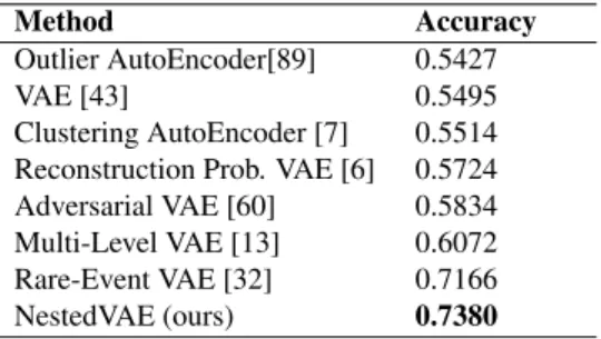
The results for the change detection task are shown in Table 2. Nested VAE is evaluated against 7 other methods, some of which are specifically designed for change detec-tion and which utilise significantly more powerful network architectures than ours [32, 13, 60]. It can be seen that Nest-edVAE outperforms the best alternative.

Method Accuracy

Outlier AutoEncoder[89] 0.5427 VAE [43] 0.5495 Clustering AutoEncoder [7] 0.5514 Reconstruction Prob. VAE [6] 0.5724 Adversarial VAE [60] 0.5834 Multi-Level VAE [13] 0.6072 Rare-Event VAE [32] 0.7166 NestedVAE (ours) 0.7380

Table 2. Change detection accuracy on rotated MNIST. L2 dis-tances between pairs of representations where images are paired according to whether they contain the same (no change) or differ-ent (change) digits. K-means clustering is then used to group the representation distances. Alternative results taken from [32]. The best result is shown inbold.

4.4. UTKFace

The UTKFace dataset [92] comprises +20k images with labels for race (White, Black, Asian, Indian, or other) and sex (male or female). Previous work has noted the bias in gender prediction software [15, 45, 64], particularly in re-lation to the accuracy of gender prediction for white indi-viduals compared to the (significantly lower) accuracy for black individuals. We note a distinction between biological sex and gender, and assume that any labels in UTKFace are actually for biological sex. This is because, despite UTK-Face referring to gender, the actual labels are for ‘male’ and ‘female’ which are terms more sensitively attributed to sex (see [17] for a discussion on the sociological aspects of gen-der).

Method ∆¯_{adj Parity (Female)} ∆¯_{adj Parity (Male)}

β-VAE 0.410 0.537

DIPVAE-I 0.394 0.547 NestedVAE (ours) 0.641 0.699

Table 3. This table shows the Adjusted Parity calculated from F1 scores across race using the UTKFace dataset. Methods with high Adjusted Parity are methods which have high F1 score for the pre-diction of biological sex and which are consistent across race. Best results are shown inbold. NestedVAE outperforms alternatives.

The dataset is first restricted to comprise only white and black individuals. This is done in order to reduce the am-biguity associated with the definition of race across ethnic-ity, as applied in UTKFace, which uses labels such as ‘In-dian’ or ’Other’. Next, the dataset is split into train and test sets, and the training set is further reduced in size such that the number of white individuals is equal to the num-ber of black individuals. We then create 5 versions of the training dataset, whereby the proportion of white individu-als is increased from 50% to 100%. The model is trained on each of these versions and embeddings for the test set are generated by passing the test set images through the trained model. Gradient boosting classifiers are used to predict sex across white and black individuals and we present the corre-sponding F1 classification scores and Area Under Receiver Operator Characteristic (AU-ROC) scores.

In terms of model parameter values, forβ-VAE,β = 4 and is annealed during training (as suggested by [33, 16]), for DIP-VAE-I,λod= 10andλd = 100. The models were

trained for 1000 epochs with an ADAM optimizer with a learning rate of 0.001 and a batch size of 64. NestedVAE had an inner latent dimensionality of 50, whilst the outer VAE had a latent dimensionality of 256. The nested and outer VAE weights γ = δ = 0.5. All alternative mod-els had a latent dimensionality of 50. A hyperparameter search yielded gradient boosting classifier parameters as follows: maximum features=50; maximum depth=5; learn-ing rate=0.25, number of estimators=300, minimum sam-ples per split=0.7. Averages and standard deviations are ac-quired over 5 runs.

UTKFace Results: The results for Adjusted Parity are shown in Table 3. These results provide a measure of con-sistency and performance (F1 score) of the classifier for the prediction of biological sex across race domains. It can be seen that NestedVAE outperforms alternatives, and also shows the smallest discrepancy in Adjusted Parity be-tween female and male classification performance (0.699 for male, compared with 0.641 for female). Notably, sex is poorly predicted using embeddings from the other mod-els. The poor prediction could be because the alternative models have embedded sex as a continuous variable (e.g. degrees of masculinity/femininity) which is entangled with other appearance dimensions, whereas NestedVAE has been explicitly trained using binary pairings of sex, thereby pro-viding significant inductive bias. The results for the Area Under Receiver Operator Characteristic (AU-ROC) score are shown in Figure 4. These results demonstrate the classi-fier performance for predicting biological sex for black indi-viduals and white indiindi-viduals using embeddings from mod-els trained on data varying in the proportion of white and black individuals. Interestingly, we do not see a large varia-tion across the training sets, suggesting that the informavaria-tion about sex encoded in the network embeddings is not

sub-stantially confounded by race. Nevertheless, NestedVAE clearly outperforms the alternative methods by a significant margin in its ability to isolate the common factors (i.e. fac-tors relating to sex).

Figure 4. Area Under Receiver Operator Characteristic (AU-ROC) scores for models trained on datasets with varying proportions of white and black individuals. NestedVAE significantly outperforms alternatives. Best viewed in color.

5. Conclusion and Further Work

NestedVAE provides a means to learn representations that are invariant to the covariates specific to domains, whilst being able to isolate the common causes across do-mains. The method combines the theory of deep latent variable VAE models with Information Bottleneck princi-ple and is trained on pairs of images with common factors and where the two images in a pair are sampled from dif-ferent domains. Results demonstrate NestedVAE’s superior performance for achieving domain invariance, change de-tection, and sex prediction. We have also presented a new (to the best of our knowledge) ‘adjusted parity metric’ in order to facilitate comparison between methods with signif-icantly different classification performance.

The principles behind NestedVAE can be applied to more exotic VAEs, and even non-VAEs. Further work should explore the application of the principles to different models.

6. Acknowledgements

This work received funding from the SNSF Sinergia project ‘SMILE’ (CRSII2 160811), the European Union’s Horizon2020 research and innovation programme under grant agreement no. 762021 ‘Content4All’ and the EPSRC project ‘ExTOL’ (EP/R03298X/1). This work reflects only the author’s view and the Commission is not responsible for any use that may be made of the information it contains.

References

[1] A. Abid and J. Zou. Contrastive variational autoencoder en-haces salient features.arXiv:1902.04601v1, 2019.

[2] A. Achille and S. Soatto. Emergence of invariance and dis-entanglement in deep representations. Journal of Machine Learning Research, 18, 2018.

[3] E. Adeli, Q. Zhao, A. Pfefferbaum, E. V. Sullivan, L. Fei-Fei, J. C. Niebles, and K. M. Pohl. Bias-resilient neural network. arXiv:1910.03676v1, 2019.

[4] A. A. Alemi, I. FIscher, J. V. Dillon, and K. Murphy. Deep variational information bottleneck. arXiv:1612.00410v7, 2017.

[5] A. A. Alemi, B. Poole, I. Fischer, J. V. Dillon, R. A. Saurous, and K. Murphy. Fixing a broken ELBO. arXiv:1711.00464v3, 2018.

[6] J. An and S. Cho. Variational autoencoder based anomaly detection using reconstruction probability.SNU Data Mining Center Tech. Report, 2015.

[7] C. Aytekin, X. Ni, F. Cricri, and E. Aksu. Clustering and unsupervised anomaly detection with L2 nrmalized deep au-toencoder representations.arXiv:1802.00187, 2018. [8] E. Banijamali, A. H. Karimi, A. Wong, and A.

Gh-odsi. Jade: Joint autoencoders for dis-entanglement. arXiv:1711.09163v1, 2017.

[9] S. Barocas, M. Hardt, and A. Narayanan. Fairness and ma-chine learning. fairmlbook.org, 2019.

[10] Y. Bengio, A. Courville, and P. Vincent. Representation learning: A review and new perspectives.IEEE Transactions on pattern analysis and machine intelligence, 2013. [11] Y. Bengio, T. Deleu, N. Rahaman, N. R. Ke, S. Lachapelle,

O. Bilaniuk, A. Goyal, and C. Pal. A meta-transfer objective for learning to disentangle causal mechanisms. arXiv:1901.10912v2, 2019.

[12] C. M. Bishop. Pattern Recognition and Machine Learning. Springer, New York, 2006.

[13] D. Bouchacourt, R. Tomioka, and S. Nowozin. Multi-level variational autoencoder: learning disentangled repre-sentations from grouped observations.arXiv:1705.08841v1, 2017.

[14] K. Bousmalis, G. Trigeorgis, N. Silberman, D. Krishnan, and D. Erhan. Domain separation networks. arXiv:1608.06019, 2016.

[15] J. Buolamwini and T. Gebru. Gender Shades: Intersec-tional accuracy disparities in commercial gender classifica-tion.Proc. of Machine Learning Research, 81:1–15, 2018. [16] C. P. Burgess, I. Higgins, A. Pal, L. Matthey, N. Watters, G.

Desjardins, and A. Lerchner. Understanding disentangling in Beta-VAE.arXiv:1804.03599v1, 2018.

[17] Y. T. Cao and H. Daume III. Toward gender-inclusive coref-erence resolution.arXiv:1910.13913v2, 2019.

[18] J. Chen and K. Batmanghelich. Robust ordinal VAE: em-ploying noisy pairwise comparisons for disentanglement. arXiv:1910.05898v1, 2019.

[19] J. Chen and K. Batmanghelich. Weakly supervised disentan-glement by pairwise similarities.arXiv:1906.01044v1, 2019. [20] T. M. Cover and J. A. Thomas.Elements of information

the-ory. John Wiley and Sons Inc., New York, 2006.

[21] E. Creager, D. Madras, J-H. Jacobsen, M. A. Weis, K. Swer-sky, T. Pitassi, and R. Zemel. Flexibly fair representation learning by disentanglement.arXiv:1906.02589v1, 2019. [22] C. Cremer, Q. Morris, and D. Duvenaud. Reinterpreting

importance-weighted autoencoders. arXiv:1704.02916v2, 2017.

[23] E. Denton and V. Birodkar. Unsupervised learning of disen-tangled representations from video.NIPS, 2017.

[24] C. Doersch. Tutorial on variational autoencoders. arXiv:1606.05908v2, 2016.

[25] Z. Feng, X. Wang, C. Ke, A. Zeng, D. Tao, and M. Song. Dual swap disentangling.32nd Conference on Neural Infor-mation Processing Systems (NeurIPS), 2018.

[26] A. Gabbay and Y. Hosen. Demystifying inter-class disentan-glement.arXiv:1906.11796v2, 2019.

[27] Y. Ganin, E. Ustinova, H. Ajakan, H. Larochelle, F. Lavio-lette, M. Marchand, and V. Lempitsky. Domain-adversarial training of neural networks.arXiv:1505.07818, 2016. [28] M. Ghifary, W. B. Kleijn, M. Zhang, and D. Balduzzi.

Do-main generalization for object recognition with multi-task autoencoders.ICCV, (2551-2559), 2015.

[29] I. Goodfellow, Y. Bengio, and A. Courville.Deep Learning. MIT Press, Cambridge, Massachusetts, 2016.

[30] I. J. Goodfellow, J. Pouget-Abadie, M. Mirza, B. Xu, D. Warde-Farley, S. Ozair, A. Courville, and Y. Bengio. Gener-ative adversarial nets.arXiv:1406.2661, 2014.

[31] N. Hadad, L. Wolf, and M. Shahar. A two-step disentangle-ment method.CVPR, 2018.

[32] R. Hamaguchi, K. Sakurada, and R. Nakamura. Rare event detection using disentangled representation learning.CVPR, 2019.

[33] I. Higgins, L. Matthey, A. Pal, C. Burgess, X. Glorot, M. Botvinick, S. Mohamed, and A. Lerchner. Beta-VAE: Learning basic visual concepts with a constrained variational framework.ICLR, 2017.

[34] M. D. Hoffman and M. J. Johnson. ELBO surgery: yet an-other way to carve up the variational evidence lower bound. 30th Conference on Neural Information Processing Systems, 2016.

[35] K. Holstein, J. W. Vaughan, H. Daume III, M. Dudik, and H. Wallach. Improving fairness in machine learning systems: what do industry practicioners need? arXiv:1812.05239v2, 2019.

[36] A. Howard and J. Borenstein. The ugly truth about ourselves and our robot creations: the problem of bias and social in-equity. Science and engineering ethics, 24(5):1521–1536, 2018.

[37] U. Hwang, J. Park, H. Jang, S. Yoon, and N. I. Cho. Pu-VAE: a variational autoencoder to purify adversarial exam-ples.arXiv:1903.00585, 2019.

[38] D. Janzing, J. Peters, J. Mooij, and B. Scholkopf. Identify-ing confounders usIdentify-ing additive noise models.Porceedings of the 25th Conference on Uncertainty in Artificial Intelligence, 2009.

[39] A. H. Jha, S. Anand, M. Singh, and V. S. R. Veeravasarapu. Disentangling factors of variational with cycle-consistent variational auto-encoders.ECCV, 2018.

[40] David A. Kenny, Deborah A. Kashy, and William L. Cook. Dyadic data analysis. Methodology in the social sciences. Guilford Press, New York, 2006.

[41] D. P. Kingma and J. L. Ba. Adam: a method for stochastic optimization.arXiv:1412.6980v9, 2017.

[42] D. P. Kingma, D. J. Rezende, S. Mohamed, and M. Welling. Semi-supervised learning with deep generative models.arXiv:1406.5298, 2014.

[43] D. P. Kingma and M. Welling. Auto-encoding variational Bayes.arXiv:1312.6114v10, 2014.

[44] J. Klys, J. Snell, and R. Zemel. Learning latent subspaces in variational autoencoders.32nd Conference on Neural Infor-mation Processing Systems (NeurIPS), 2018.

[45] A. Kortylewski, B. Egger, A. Morel-Forster, A. Schneider, T. Gerig, C. Blumer, C. Reyneke, and T. Vetter. Can synthetic faces undo the damage of dataset bias to face recognition and facial landmark detection?arXiv:1811.08565v2, 2019. [46] T. D. Kulkarni, W. Whitney, P. Kohli, and J. B.

Tenen-baum. Deep convolutional inverse graphics network. arXiv:1503.03167v4, 2015.

[47] A. Kumar, P. Sattigeri, and A. Balakrishnan. Variational in-ference of disentangled latent concepts from unlabeled ob-servations.arXiv:1711.00848v3, 2018.

[48] G. Lample, N. Zeghidour, N. Usunier, A. Bordes, L. De-noyer, and M.A. Ranzato. Fader networks: Manipulating images by sliding attributes.arXiv:1706.00409, 2018. [49] Y. LeCun, C. Cortes, and C. J. Burges. MNIST handwritten

digit database.AT&T Labs, 2010.

[50] C. M. Lee, C. Hart, J. G. Richens, and S. Johri. Leveraging directed causal discovery to detect latent common causes. arXiv:1910.10174v1, 2019.

[51] H.Y. Lee, H.Y. Tseng, J.B. Huang, M. Singh, and M.H. Yang. Diverse image-to-image translation via disentangled repre-sentations.arXiv:1808.00948, 2018.

[52] J. Lezama. Overcoming the disentanglement vs reconstruc-tion trade-off via Jacobian supervision.ICLR, 2019. [53] H. Liu, J. Dacon, W. Fan, H. Liu, and J. Liu, Z.and Tang.

Does gender matter? towards fairness in dialogue systems. arXiv:1910.10486v1, 2019.

[54] M. llse, J. M. Tomczak, C. Louizos, and M. Welling. DIVA: domain invariant variational autoencoders. arXiv:1905.10427, 2019.

[55] F. Locatello, G. Abbati, T. Rainforth, T. Bauer, S. Bauer, B. Scholkopf, and O. Bachem. On the fairness of disentangled representations.arXiv:1905.13662v1, 2019.

[56] F. Locatello, S. Bauer, M. Lucic, G. Ratsch, S. Gelly, B. Scholkopf, and Bachem O. Challenging common assump-tions in the unsupervised learning of disentangled represen-tations.arXiv:1811.12359v3, 2019.

[57] C. Louizos, K. Swersky, Y. Li, M. Welling, and R. Zemel. The variational fair autoencoder.arXiv:1511.00830, 2017. [58] C. Louizos and M. Welling. Structured and efficient

variational deep learning with matrix Gaussian posteriors. arXiv:1603.04733v5, 2016.

[59] T. Lucas and J. Verbeek. Auxiliary guided autoregressive variational autoencoders.arXiv:1711.11479, 2018.

[60] M. Mathieu, J. Zhao, P. Sprechmann, A. Ramesh, and Y. Le-Cun. Disentangling factors of variation in deep representa-tions using adversarial training.arXiv:1611.03383v1, 2016. [61] P.A. Mattei and J. Frellsen. Leveraging the exact likelihood of deep latent variable models.arXiv:1802.04826v4, 2018. [62] L. McInnes and J. Healy. UMAP: uniform manifold

approximation and projection for dimension reduction. arXiv:1802.03426v1, 2018.

[63] N. Mehrabi, F. Morstatter, N. Saxena, K. Lerman, and A. Galstyan. A survey on bias and fairness in machine learning. arXiv:1908.09635, 2019.

[64] M. Merler, N. Rather, R. Feris, and J. R. Smith. Diversity in faces.arXiv:1901.10436v6, 2019.

[65] D. Moyer, S. Gao, R. Brekelmans, G. V. Steeg, and A. Gal-styan. Invariant representations without adversarial training. NeurIPS, 2018.

[66] R. Nabi, D. Malinsky, and I. Shpitser. Optimal training of fair predictive models.arXiv:1910.04109v1, 2019. [67] Y. Netzer, T. Wang, A. Coates, A. Bissacco, B. Wu, and A. Y.

Ng. Reading digits in natural iages with unsupervised feature learning.NIPS, 2011.

[68] B. T. M. Phuong, N. Kushman, S. Nowozin, R. Tomioka, and M. Welling. The mutual autoencoder: controlling informa-tion in latent code representainforma-tions.ICLR, 2018.

[69] O. Press, T. Galatni, S. Benaim, and L Wolf. Emerging disen-tanglement in auto-encoder based unsupervised image con-tent transfer.ICLR, 2019.

[70] D. J. Rezende, S. Mohamed, and D. Wierstra. Stochastic backpropagation and approximate inference in deep genera-tive models.arXiv:1401.4082, 2014.

[71] A. Rose. Are face-detection cameras racist? Time Business, 2010.

[72] A. Ruiz, O. Martinez, X. Binefa, and J. Verbeek. Learn-ing disentangled representations with reference-based varia-tional autoencoders.arXiv:1901.08534v1, 2019.

[73] A. Sepliarskaia, J. Kiseleva, and M. de Rijke. Evaluating disentangled representations.arXiv:1910.05587v1, 2019. [74] S. Shankar, V. Piratla, S. Chakrabarti, S. Chaudhuri, P.

Jyothi, and S. Sarawagi. Generalizing across domains via cross-gradient training.arXiv:1804.10745.v2, 2018. [75] R. Shu, Chen Y., A. Kumar, S. Ermon, and B.

Poole. Weakly supervised disentanglement with guarantees. arXiv:1910.09772v1, 2019.

[76] N. Siddharth, B. Paige, V. de Meent, A. Desmaison, F. Wood, N. D. Goodman, P. Kohli, and P. H. Torr. Learning disen-tangled representations with semi-supervised deep genera-tive models.arXiv:1706.00400, 2017.

[77] D. Slack, S. Hilgard, E. Jia, S. Singh, and H. Lakkaraju. How can we fool LIME and SHAP? adversarial attacks on post hoc explanation methods.arXiv:1911.02508v1, 2019. [78] C. K. Sonderby, T. Raiko, L. Maaloe, S. K. Sonderby, and

O Winther. How to train deep variational autoencoders and probabilistic ladder networks.arXiv:1602.02282v1, 2016. [79] R. Suter, D. Miladinovic, S. Bauer, and B. Scholkopf.

Interventional robustness of deep latent variable models. arXiv:1811.00007v1, 2018.

[80] A. Szabo, Q. Hu, T. Portenier, and P. Favaro. Chal-lenges in disentangling independent factors of variation. arXiv:1711.02245v1, 2017.

[81] A. Szabo, Q. Hu, T. Portenier, M. Zwicker, and P. Favaro. Understanding degeneracies and ambiguities in attribute transfer.ECCV, 2018.

[82] N. Tishby, F. C. Pereira, and W. Bialek. The information bottleneck method.arXiv:physics/0004057v1, 2000. [83] N. Tishby and N. Zaslavsky. Deep learning and the

informa-tion bottleneck principle.arXiv:1503.02406v1, 2015. [84] J. M. Tomczak and M. Welling. VAE with a VampPrior.

arXiv:1705:07120v5, 2018.

[85] M. Tschannen, O. Bachen, and M. Lucic. Recent advances in autoencoder-based representation learning. arXiv:1812.05069v1, 2018.

[86] L. van der Maaten and G. E. Hinton. Visualizing data using t-SNE.Journal of Machine Learning Research, 9:2579–2605, 2008.

[87] M. J. Vowels, N. C. Camgoz, and R. Bowden. Gated vari-ational autoencoders: Incorporating weak supervision to en-courage disentanglement.arXiv:1911.06443v1, 2019. [88] H. Wang, Z. He, Z. C. Lipton, and E. P. Xing. Learning

robust representations by projecting supervicial statistics out. ICLR, 2019.

[89] Y. Xia, X. Cao, F. Wen, G. Hua, and J. Sun. Learning dis-criminative reconstructions for unsupervised outlier removal. ICCV, 2015.

[90] Q. Xie, Z. Dai, Y. Du, E. Hovy, and G. Neubig. Con-trollable invariance through adversarial feature learning. arXiv:1705.1122v3.

[91] R. Zemel, Y. L. Wu, K. Swersky, T. Pitassi, and C. Dwork. Learning fair representations.Proc. of the 30th International Conference on Machine Learning, 28, 2013.

[92] Z. Zhang, Y. Song, and H. Qi. Age progression/regression by conditional adversarial autoencoder. arXiv:1702.08423, 2017.

[93] S. Zhao, J. Song, and S. Ermon. InfoVAE: Balanc-ing learnBalanc-ing and inference in variational autoencoders. arXiv:1706.02262v3, 2018.

[94] Sun Zheng. Disentangling latent space for VAE by label rel-evant/irrelevant dimensions.CVPR, 2018.