Consistent community detection in uni-layer and multi-layer networks

c

CONSISTENT COMMUNITY DETECTION IN UNI-LAYER AND MULTI-LAYER NETWORKS

BY

SUBHADEEP PAUL

DISSERTATION

Submitted in partial fulfillment of the requirements for the degree of Doctor of Philosophy in Statistics

in the Graduate College of the

University of Illinois at Urbana-Champaign, 2017

Urbana, Illinois

Doctoral Committee:

Professor Yuguo Chen, Chair, Director of Research Professor Xiaohui Chen

Professor Bruce Hajek Professor Stephen Portnoy Professor Douglas Simpson

Abstract

Over the last two decades, we have witnessed a massive explosion of our data collection abilities and the birth of a “big data” age. This has led to an enormous interest in statistical inference of a new type of complex data structure, a graph or network. The surge in interdisciplinary interest on statistical analysis of network data has been driven by applications in Neuroscience, Genetics, Social sciences, Computer science, Economics and Marketing. A network consists of a set of nodes or vertices, representing a set of entities, and a set of edges, representing the relations or interactions among the entities. Networks are flexible frameworks that can model many complex systems.

In the majority of the network examples dealt with in the literature, the relations between nodes are assumed to be of the same type such as web page linkage, friendship, co-authorship or protein-protein interaction. However, the complex networks in many modern applications are often multi-layered in the sense that they consist of multiple types of edges/relations among a group of entities. Each of those different types of relations can be viewed as creating its own network, called a layer of the multi-layer network. Multi-layer networks are a more accurate representation of many complex systems since many entities in those systems are involved simultaneously in multiple interactions. In this dissertation we view multi-layer networks in the broad sense that includes multiple types of relations as well as multiple information sources on the same set of nodes (e.g., multiple trials or multiple subjects).

The problem of detecting communities or clusters of nodes in a network has received considerable attention in literature. As with uni-layer networks, community detection is an important task in multi-layer networks. This dissertation aims to develop new methods and theory for community detection in both uni-layer and multi-layer networks that can be used to answer scientific questions from experimental data.

statistical random graph models, (2) based on maximizing quality functions, e.g., the modularity score and (3) based on spectral and matrix factorization methods.

In Chapter 2 we consider two random graph models for community detection in multi-layer networks, the multi-layer stochastic blockmodel (MLSBM) and a model with a restricted parameter space, the restricted multi-layer stochastic blockmodel (RMLSBM). We derive consistency results for community assignments of the maximum likelihood estimators (MLEs) in both models where MLSBM is assumed to be the true model, and either the number of nodes or the number of types of edges or both grow. We compared MLEs in the two models among themselves and with other baseline approaches both theoretically and through simulations. We also derived minimax error rates and thresholds for achieving consistency of community detection in MLSBM, which were then used to show the advantage of the multi-layer model over a traditional alternative, the aggregate stochastic block model. In simulations RMLSBM is shown to have advantage over MLSBM when either the growth rate of the number of communities is high or the growth rate of the average degree of the component graphs in the multi-graph is low.

A popular method of community detection in uni-layer networks is maximization of a partition quality function called modularity. In Chapter 3 we introduce several multi-layer network modu-larity measures based on different random graph null models, motivated by empirical observations from a diverse field of applications. In particular, we derived different modularities by defining the multi-layer configuration model, the multi-layer expected degree model and their various modifi-cations as null models for multi-layer networks. These measures are then optimized to detect the optimal community assignment of nodes. We apply the methods to five real multi-layer networks - three social networks from the website Twitter, a complete neuronal network of a nematode,

C-elegans and a classroom friendship network of 7th-grade students.

In Chapter 4 we present a method based on the orthogonal symmetric non-negative matrix tri-factorization of the normalized Laplacian matrix for community detection in complex networks. While the exact factorization of a given order may not exist and is NP hard to compute, we obtain an approximate factorization by solving an optimization problem. We establish the connection of the factors obtained through the factorization to a non-negative basis of an invariant subspace of the estimated matrix, drawing parallel with the spectral clustering. Using such factorization

for clustering in networks is motivated by analyzing a block-diagonal Laplacian matrix with the blocks representing the connected components of a graph. The method is shown to be consistent for community detection in graphs generated from the stochastic block model and the degree corrected stochastic block model. Simulation results and real data analysis show the effectiveness of these methods under a wide variety of situations, including sparse and highly heterogeneous graphs where the usual spectral clustering is known to fail. Our method also performs better than the state of the art in popular benchmark network datasets, e.g., the political web blogs and the karate club data.

In Chapter 5 we once again consider the problem of estimating a consensus community structure by combining information from multiple layers of a multi-layer network or multiple snapshots of a time-varying network. Numerous methods have been proposed in the literature for the more general problem of multi-view clustering in the past decade based on the spectral clustering or a low-rank matrix factorization. As a general theme, these “intermediate fusion” methods involve obtaining a low column rank matrix by optimizing an objective function and then using the columns of the matrix for clustering. Such methods can be adapted for community detection in multi-layer networks with minimal modifications. However, the theoretical properties of these methods remain largely unexplored and most authors have relied on performance in synthetic and real data to assess the goodness of the procedures. In the absence of statistical guarantees on the objective functions, it is difficult to determine if the algorithms optimizing the objective will return a good community structure. We apply some of these methods for consensus community detection in multi-layer networks and investigate the consistency properties of the global optimizer of the objective functions under the multi-layer stochastic blockmodel. We derive several new asymptotic results showing consistency of the intermediate fusion techniques along with the spectral clustering of mean adjacency matrix under a high dimensional setup where both the number of nodes and the number of layers of the multi-layer graph grow. We complement the asymptotic analysis with a thorough numerical study to compare the finite sample performance of the methods.

Motivated by multi-subject and multi-trial experiments in neuroimaging studies, in Chapter 6 we develop a modeling framework for joint community detection in a group of related networks. The proposed model, which we call the random effects stochastic block model facilitates the study

of group differences and subject specific variations in the community structure. In contrast to the previously proposed multi-layer stochastic block models, our model allows community memberships of nodes to vary in each component network or layer with a transition probability matrix, thus modeling the variation in community structure across a group of subjects or trials. We propose two methods to estimate the parameters of the model, a variational-EM algorithm and two non-parametric “two-step” methods based on spectral and matrix factorization respectively. We also develop several hypothesis tests with p-values obtained through resampling (permutation test) for differences in community structure in two groups of subjects both at the whole network level and node level. The methodology is applied to publicly available fMRI datasets from multi-subject experiments involving schizophrenia patients along with healthy controls. Our methods reveal an overall putative community structure representative of the groups as well as subject-specific variations within each group. Using our network level hypothesis tests we are able to ascertain statistically significant difference in community structure between the two groups, while our node level tests help determine the nodes that are driving the difference.

Acknowledgments

This dissertation would not have been possible without the help of numerous people. First I would like to thank my advisor, Prof. Yuguo Chen for encouraging me to explore and seek answers to challenging problems and guiding me through the intricacies of those problems. I am immensely grateful to him for reading through and correcting the component manuscripts several times that has improved the quality of the document. I also thank all the doctoral committee members, Prof. Bruce Hajek, Prof. Douglas Simpson, Prof. Stephen Portnoy and Prof. Xiaohui Chen who offered feedback, guidance and support. Many thanks to the Department of statistics at the the University of Illinois, Urbana-Champaign for the support and encouragement that I have received from everyone here. Also, thanks to all the faculty and my fellow Ph.D students from whom I have learned a great deal. In particular, I am grateful to former fellow Ph.D student Prof. Srijan Sengupta for many stimulating discussions. And finally, I would like to thank my parents for the countless sacrifices they have made to enable me to pursue my doctoral studies which eventually led to this dissertation.

Table of Contents

List of Tables . . . xi

List of Figures. . . xii

List of Abbreviations . . . xv

Chapter 1 Introduction . . . 1

1.1 Multi-layer networks . . . 1

1.2 Community structure in uni-layer and multi-layer networks . . . 3

1.3 Groups of networks in neuroimaging studies . . . 9

Chapter 2 Community detection in multi-layer networks through multi-layer stochastic blockmodel . . . 12

2.1 Extension of blockmodels to multi-layer settings . . . 12

2.2 Consistency . . . 15

2.2.1 Preliminaries . . . 17

2.2.2 Main results. . . 21

2.2.3 Sparse networks . . . 27

2.2.4 A Large number of communities . . . 27

2.3 Baseline procedures. . . 28

2.4 Minimax rates and consistency thresholds . . . 29

2.4.1 Consistency thresholds. . . 33

2.5 Estimation using mixture model approach . . . 34

2.6 Hypothesis testing for multi-layer network modeling . . . 36

2.7 Simulation results . . . 37

2.7.1 FixedK and M whileN increases . . . 39

2.7.2 FixedN andM whileK increases . . . 41

2.7.3 FixedN andK while M increases . . . 41

2.7.4 Computing time . . . 43

2.8 Twitter UK politics dataset . . . 43

2.9 Discussions . . . 46

2.10 Proofs and derivations . . . 47

2.10.1 Derivation of variational inference for RMLSBM . . . 47

2.10.2 Proof of Equation (2.2.16) . . . 48

2.10.3 Proofs of consistency results. . . 49

Chapter 3 Null models and modularity based community detection in

multi-layer networks . . . 81

3.1 Multi-layer networks . . . 81

3.1.1 Null models for community detection. . . 82

3.1.2 Degrees in multi-layer network and null models . . . 84

3.1.3 Null model selection . . . 85

3.2 Multi-layer configuration models and modularities . . . 88

3.3 Degree corrected multi-layer stochastic blockmodel . . . 90

3.3.1 Modularities based on Multi-layer stochastic blockmodels . . . 93

3.4 Computation . . . 97

3.5 Simulation results . . . 98

3.5.1 Data generation . . . 99

3.5.2 Number of communities unknown. . . 100

3.5.3 Number of communities known . . . 103

3.6 Real data analysis . . . 104

3.6.1 Twitter datasets . . . 105

3.6.2 C-elegans . . . 108

3.6.3 Grade 7 students network . . . 110

3.7 Conclusions . . . 112

Chapter 4 Orthogonal symmetric non-negative matrix factorization under stochas-tic block model . . . 115

4.1 Introduction . . . 115

4.2 Methods and algorithms . . . 116

4.2.1 Another characterization of approximate OSNTF . . . 120

4.2.2 Uniqueness . . . 121

4.3 Motivation and connection with spectral clustering . . . 121

4.3.1 Connections to invariant subspaces and projections . . . 121

4.3.2 Motivation through block diagonal matrix . . . 123

4.4 Consistency of OSNTF for community detection . . . 124

4.4.1 Recovery . . . 126

4.4.2 Uniform convergence of objective function . . . 127

4.4.3 Characterizing mis-clustering . . . 130

4.4.4 Application to four parameter SBM . . . 133

4.5 Simulation Results . . . 133

4.5.1 SBM : increasing degrees . . . 135

4.5.2 SBM : increasing nodes . . . 135

4.5.3 DCSBM : varying degree parameter . . . 135

4.6 Real data analysis . . . 136

4.6.1 Political blogs data . . . 136

4.6.2 Karate club dataset . . . 137

4.6.3 Dolphins dataset . . . 138

4.7 Discussions . . . 138

4.8 Proofs . . . 139

4.8.1 Proof of Lemma 10 and Corollary 1 . . . 139

4.8.2 Proof of Lemma 11 . . . 140

4.8.4 Proof of Lemma 12 . . . 141 4.8.5 Proof of Lemma 13 . . . 142 4.8.6 Proof of Lemma 14 . . . 143 4.8.7 Proof of Lemma 15 . . . 144 4.8.8 Proof of Theorem 9 . . . 145 4.8.9 Proof of Lemma 16 . . . 146 4.8.10 Proof of Lemma 17 . . . 147

Chapter 5 Consistency of community detection in multi-layer networks using spectral and matrix factorization methods . . . 149

5.1 Introduction . . . 149

5.2 Methods and algorithms . . . 151

5.2.1 Linked matrix factorization. . . 151

5.2.2 Co-regularized spectral clustering. . . 153

5.2.3 Spectral clustering on mean adjacency matrix . . . 154

5.2.4 Aggregate spectral kernel and module allegiance matrix . . . 155

5.3 Models and mis-clustering . . . 156

5.3.1 Correct recovery in the noiseless case. . . 157

5.3.2 Characterizing mis-clustering . . . 158 5.4 Consistency results . . . 159 5.5 Simulation studies . . . 164 5.6 Conclusion . . . 170 5.7 Proofs . . . 171 5.7.1 Proof of Proposition 3 . . . 171 5.7.2 Proof of Lemma 18 . . . 171 5.7.3 Proof of Theorem 11 . . . 172 5.7.4 Proof of Theorem 12 . . . 175 5.7.5 Proof of Lemma 19 . . . 178 5.7.6 Proof of Theorem 13 . . . 179 5.7.7 Proof of Theorem 14 . . . 182 5.7.8 Proof of Lemma 20 . . . 182

Chapter 6 A random effects stochastic block model for joint community detec-tion in multiple networks with applicadetec-tions to neuroimaging . . . 183

6.1 Models for multi-layer networks with community structure . . . 183

6.2 Random effects multi-layer stochastic block model . . . 185

6.3 A variational EM estimator . . . 188

6.4 Two-step spectral/NMF and ML algorithm . . . 191

6.4.1 Co-regularized spectral clustering algorithm . . . 191

6.4.2 Co-regularized orthogonal non-negative matrix tri factorization algorithm . . 192

6.4.3 The conditional ML step. . . 195

6.5 Two-sample hypothesis testing: whole network-level and node-level tests . . . 196

6.6 Performance on simulated networks. . . 199

6.6.1 Methods compared . . . 200

6.6.2 Increasing variation across layers . . . 201

6.6.3 Increasing number of layers . . . 202

6.6.5 Performance of hypothesis testing procedures on synthetic networks . . . 204

6.7 Application to a resting state fMRI neuroimaging study on schizophrenia . . . 207

6.7.1 COBRE dataset . . . 207

List of Tables

2.1 Average degrees of nodes in different network layers for Twitter UK politics data . . 44 2.2 The NMI and CCR for Twitter UK politics data . . . 46 3.1 The number of communities detected and the NMI of clustering for different

com-munity detection methods for Twitter UK politics data. The comcom-munity names are identified by optimal assignment. . . 106 3.2 The NMI of clustering from different community detection methods for Twitter

Irish politics data. The community names are identified by optimal assignment, “no. comm.” stands for number of communities detected. . . 107 3.3 Performance of different community detection methods in terms of (a) number of

clusters detected and NMI of clustering, and (b) NMI of clustering with known number of communities for Twitter English Premier League dataset . . . 109 3.4 NMI of clustering with the gender-wise clusters assumption for 7th grade students

peer network; (a) Number of clusters detected and NMI of clustering and (b) NMI of clustering with number of clusters given as 2.. . . 113 4.1 Comparison of the methods in terms of the number of times a method performs the

best in the simulations . . . 136 4.2 Comparison of NMF with other methods in terms of the number of nodes

mis-classified and the NMI with the ground truth in the political blogs dataset. . . 137 6.1 Network level tests: p-values of various test statistics on two synthetic network

sam-ples of size 20 and 25 drawn from a 100-node, 3-community RESBM. The columns represent results for different fraction of nodes that were changed to obtain the second ¯Z from the first. 10000 resamples was used to compute the p-values, a * indicates significant at 1% level . . . 205 6.2 Performance of node level tests (total errors and false positives) on testing between

two samples of synthetic networks of size 20 and 25 drawn from a 100-node, 3-community RESBM: (a) at 0.05 FWER threshold, (b) at 0.05 FDR threshold and (c) at 0.10 FDR threshold. Number of nodes changed is the actual number of nodes whose mean putative community assignment varied between the two groups.. . . 206 6.3 Average modularity and average number of communities detected by modularity

maximization (Spinglass and Louvain methods) in the two groups of subjects for different thresholds. The columns of p-value indicate p-value obtained from Welch two sample t-test for difference in means. A * indicates statistically significant at 5% level . . . 208 6.4 Nodes of Interest: Nodes which are significant at 0.1 FDR correction. . . 210

List of Figures

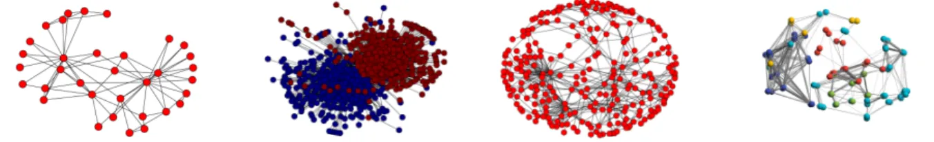
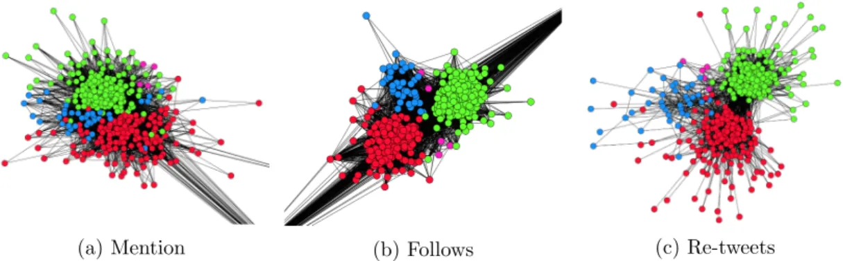
1.1 Networks: (a) Friendship patterns in a karate club (Zachary, 1977); (b) Hyperlinks between political blogs (Adamic and Glance, 2005); (c) Electrical synapses in the nervous system of C-elegans; (d) Functional connectivity network of brain regions from AAL Atlas measure through fMRI. . . 1 1.2 A 3-layer twitter network of British MPs. The nodes are colored according to an

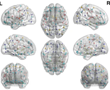
underlying community structure: the party memberships. . . 3 1.3 Political Blogs data: Nodes grouped according to communities detected . . . 4 1.4 Mean community structure in the functional network of brain regions in a group

of 70 healthy subjects. Nodes : Regions of interest from AAL atlas, colored by communities. Edges : Mean functional connectivity. . . 9 2.1 Comparison of the performance of various methods for three simulation settings under two

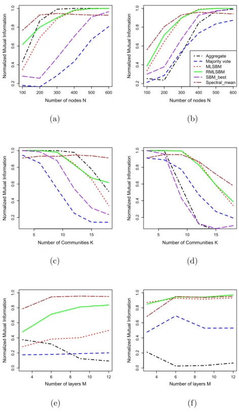
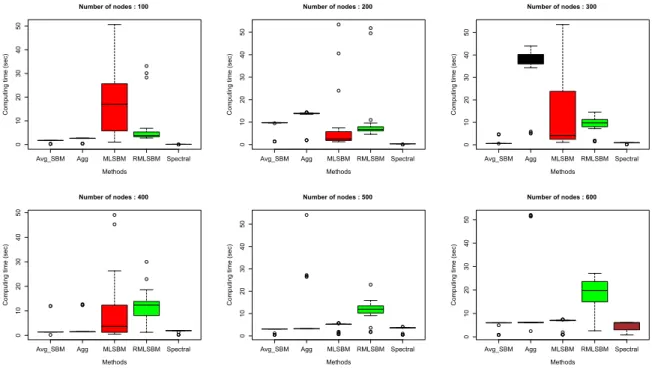
scenarios: all layers are sparse and have strong SNR (left column: (a)(c)(e)), and the layers are mixed in terms of sparsity and SNR (right column: (b)(d)(f)). (a, b) fixed K = 10 and M = 5 while N increases from 100 to 600; (c, d) fixed N = 400 and M = 5 whileK increases from 3 to 18; (e, f) fixed N = 300 and K = 15 while M increases from 3 to 12. The legend in Figure (b) is common to all figures. SBM best indicates the result from the best performing MLE in the single layer SBMs. . . 40 2.2 Comparison of the computing time of various methods for increasing number of nodes under

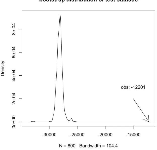
the scenario that all layers are sparse and have strong SNR with fixed K= 10 andM = 5 whileN increases from 100 to 600; . . . 44 2.3 The parametric bootstrap distribution (based on 800 samples) of the log likelihood

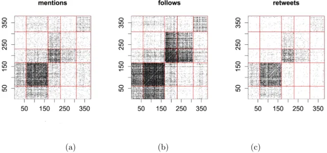
ratio test statistic. The observed value of the statistic is marked. . . 77 2.4 The adjacency matrices of the three layers: (a) mentions, (b) follows and (c) retweets,

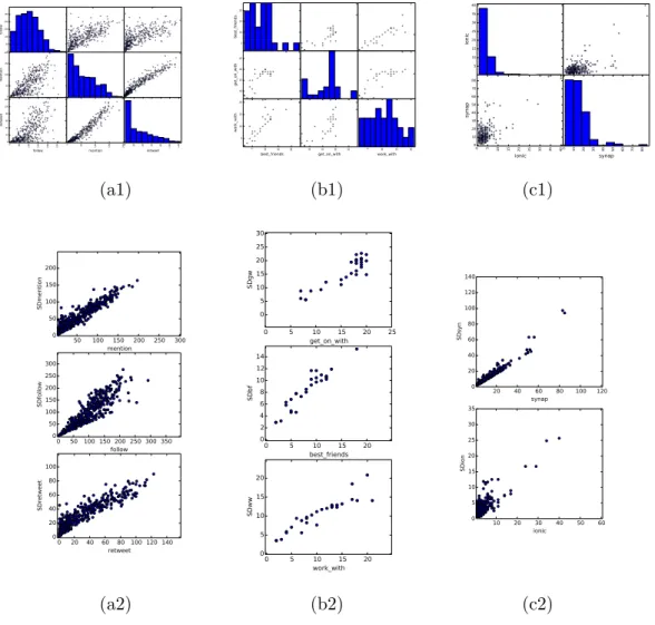
sorted according to the common community labels obtained from maximum likeli-hood estimation in RMLSBM. The colored grid lines indicate community partitions. 78 3.1 Observed degree distributions across layers in (a1) Twitter network of British MPs,

(b1) 7th grade school students and (c1) C-elegans neuronal network; (a2, b2, c2) degree distribution fitted with a shared degree model plotted as scatter plots with the observed degrees in each layer. . . 86

3.2 Comparison of the performance of various multi-layer modularities for data generated from the DCBM with independent degrees. The layers are sparse and the signal is strong across all layers. (a) The number of nodes and number of communities are fixed at 800 and 3 while the average degree of the nodes across all layers combined is increased. (b) The number of nodes is increased from 300 to 600 while the number of communities is fixed at 3. In both cases, the top figure is the comparison in terms of NMI of the community assignment and the bottom figure is the box plot of the number of communities detected. . . 101 3.3 Comparison of the performance of various multi-layer modularities for data generated

from the independent degree DCBM. Both sparsity and signal quality are mixed across different layers. (a)N andK are fixed at 800 and 3 while the average degree of the nodes across all layers combined is increased. (b) Increasing nodes with fixed K = 3. (c) Increasing number of communities with fixed N = 800. In all cases, the left side figure is the comparison in terms of NMI and the right side figure is the box plot of the number of communities detected. . . 102 3.4 Comparison of performance with known number of communities of various MLED

modularities along with MNavrg for data generated from the stochastic blockmodel. The layers are mixed in sparsity and signal quality. The average degree on nodes across all layers are increasing while N,K and M are fixed at 500, 2 and 4 respec-tively. We consider two cases: (a) balanced community sizes (roughly half of the nodes belonging to either cluster), and (b) unbalanced community sizes (30% of the nodes belonging to one cluster and 70% belonging to the other). . . 104 3.5 Parametric bootstrap distribution of the likelihood ratio test statistic for (a)

C-elegans network and (b) Grade 7 students network. The observed value of the test statistic is indicated with an arrow. . . 110 3.6 Adjacency matrices of the 2 layers in C-elegans connectome, (a) ionic channel and

(b) chemical synapse, sorted and marked according to the clustering results obtained from SDlocal. . . 110 3.7 Adjacency matrices of the 2 layers in C-elegans connectome, (a) ionic channel and

(b) chemical synapse, sorted and marked according to the clustering results obtained from MNavrg. . . 111 3.8 Adjacency matrices of the three layers, (a) get on with, (b) best friends and (c) work

with, sorted and marked according to the (same) clustering result obtained from SDlocal, SDratio and MNavrg. . . 112 4.1 Comparison of the performance of various methods for three simulation settings: (a) SBM

with N = 800, K = 3 and increasing average degree, (b) SBM withK = 3 and increasing number of nodes, and (c) DCSBM withN = 600,K= 3 and decreasing degree heterogeneity. The legend in Figure (a) is common to all figures. . . 134 5.1 Performance of various methods with increasing average degree of nodes for data

generated from MLSBM with 600 nodes, 5 layers and 3 communities. (a) All layers have strong signals with some variations; (b) the layers are mixed in terms of signal quality. . . 166 5.2 Performance of various methods with (a) increasing average degree of nodes for data

generated from MLSBM with 600 nodes, 5 layers and 3 communities, (b) increasing number of layers with 300 nodes and 6 communities. The labels in Figure (b) is shared for both figures.. . . 167

5.3 Performance of various methods with (a) increasing average degree of nodes for data generated from MLSBM with 600 nodes, 5 layers and 3 communities, where 3 layers contain homophilic clusters and the other 2 contain heterophilic clusters . . . 168 6.1 Schematic diagram of the RESBM . . . 186 6.2 Performance of of various methods across three metric, (a) Average clustering

perfor-mance across all layers (in NMI), (b) perforperfor-mance in detecting the mean community structure (in NMI) and (c) accuracy in estimating the transition probability matrix (in Frobenius norm) with increasing variation factor from 0.05 to 0.40. The number of nodes is 500, the number of communities is 3, the number of layers is 5 and the average degree per layer is 40. . . 201 6.3 Performance of of various methods across three metric, (a) Average clustering

perfor-mance across all layers (in NMI), (b) perforperfor-mance in detecting the mean community structure (in NMI) and (c) accuracy in estimating the transition probability matrix (in Frobenius norm) with increasing number of layers from 5 to 25. The number of nodes is 300, the number of communities is 3, the average degree per layer is 25, and the variation factor is 0.20. . . 202 6.4 Performance of of various methods across three metric, (a) Average clustering

perfor-mance across all layers (in NMI), (b) perforperfor-mance in detecting the mean community structure (in NMI) and (c) accuracy in estimating the transition probability matrix (in Frobenius norm) with increasing average degree per layer from 30 to 70. Number of nodes is 500, number of communities is 3, number of layers is 5 and the variation factor is 0.20. . . 203 6.5 Group putative community structure of resting state network based on AAL ROIs

in (a, c, e) healthy controls, and (b, d, f) patients with schizophrenia. Nodes are colored according to their group putative community obtained from the following methods: Co-Spectral for the first row (a, b), Co-OSNTF for the second row (c, d) and VarEM for the third row (e, f).. . . 209 6.6 A visualization of the group putative community structure in healthy controls and

patients. . . 212 6.7 Stability of the group putative community assignments for VarEM : (a) and (b) are

the matrices with elements as fraction of subjects for which two nodes (ROIs) are in the same community sorted according to the putative community structure for healthy controls and patients respectively; (c) and (d) are the estimated transition matrices among modules for healthy controls and patients respectively. . . 213 6.8 Group putative community structure of resting state network from Co-OSNTF. In

(a) the edges represent fraction of subjects for which two nodes are in the same community with a threshold of 0.40, while in (b) the edges represent the average connectivity (correlation) between two nodes across all subjects with a threshold of 0.50. In each case nodes are colored according to their group putative community in (L) Controls and (R) Patients. . . 213

List of Abbreviations

SBM Stochastic block model

DCSBM Degree corrected stochastic block model NMF Non-negative matrix factorization

SNMF Symmetric non-negative matrix factorization

OSNTF Orthogonal symmetric non-negative matrix factorization MLSBM Multi-layer stochastic blockmodel

RMLSBM Restricted multi-layer stochastic blockmodel MLE Maximum likelihood estimate

RMLE Restricted maximum likelihood estimate MLCM Multi-layer configuration model

Co-OSNTF Co-regularized orthogonal symmetric non-negative matrix factorization OLMF Orthogonal linked matrix factorization

RESBM Random effects stochastic block model

Chapter 1

Introduction

Over the last decade, relational data has become ubiquitous in all forms of human activities. In many applications of statistics and machine learning, one encounters relational data where the entities are represented as nodes or vertices and the relations or interactions between the entities as edges of a graph. Applications of such graphs or networks include many information systems such as social networks, World Wide Web, user information databases in e-commerce, metabolic networks, gene regulatory networks, protein-protein interaction networks, neuronal networks and food web. Some examples of networks are presented in Figure1.1.

1.1

Multi-layer networks

In majority of the cases dealt with in the literature, the relations are assumed to be of the same type such as web page linkage, friendship, co-authorship and protein-protein interaction. How-ever in modern complex relational databases and networks, we often have information regarding relationships of multiple types among the nodes. Such multi-relational data can be represented as multi-layer graphs where multiple types of edges represent the relations and the set of vertices/nodes

Figure 1.1: Networks: (a) Friendship patterns in a karate club (Zachary, 1977); (b) Hyperlinks between political blogs (Adamic and Glance, 2005); (c) Electrical synapses in the nervous system of C-elegans; (d) Functional connectivity network of brain regions from AAL Atlas measure through fMRI.

represents the entities [75].

Each of those different types of relation can be viewed as creating its own network, called a “layer” of the multi-layer network. Multi-layer networks are a more accurate representation of many complex systems since many entities in those systems are involved simultaneously in multiple networks. This means each of the individual network carries only partial information about the interactions among the entities and full information is available only through the multi-layer networked system [134,120]. We will consider a number of such inherently multi-plex networks as real world examples in this thesis. In the social networking website Twitter, users can engage in various types of interactions with other users, e.g “mention”, “follow”, “retweet” etc. [63, 120]. Although, the individual network layers created by these relationships are structurally highly related, they represent different facets of user behavior and ignoring the differences might lead to spurious conclusions. In another example from biology, the neural network of a small organism, Caenorhabditis elegans, consist of neurons which are connected to each other by two types of connections, a synaptic (chemical) link and an ionic (electrical) link. The two types of links have markedly different dynamics and hence should be treated as two separate layers of a network instead of fusing together into a single network [21]. See [82,21,117] for more examples and discussions of multi-layer networks.

We assume that such networks have an implicit community structure and different observed layers manifest that underlying structure with varying amount of information and noise. As an example of a network where such an assumption is reasonable, we analyze a twitter network of British Members of Parliament (see Figure 1.2) where the underlying communities are based on their party memberships and the three observed layers, “mentions”, “follows” and “’re-tweets” manifest that structure in varying proportions. In such cases the multi-layer graph is a more accurate representation of the underlying similarity of the objects and each layer can provide only “partial” information about the data [134]. The goal in such cases would be to correctly identify the underlying set of communities combining information from all three layers.

Earlier approaches towards multi-relational data or multi-layer graph clustering suffer from the deficiency that they either cluster each graph independently and combine the results, or aggregate the graphs and cluster the aggregated graph. These approaches fail to take into account the

de-(a) Mention (b) Follows (c) Re-tweets

Figure 1.2: A 3-layer twitter network of British MPs. The nodes are colored according to an underlying community structure: the party memberships.

pendency among the different layers, in particular the correlation among different types of edges that share the same pair of nodes. Moreover, the multiple network layers can have different charac-teristics in terms of sparsity and noise. Some layers may be dense but may carry little worthwhile information, whereas some layers may be extremely sparse but may carry valuable information. The aggregation process of graphs could lose the intrinsic heterogeneity of the network layers. Here we attempt to address the problem of how to efficiently cluster the nodes or entities in a network taking into account all types of layers or relations among them. Several approaches have been recently proposed in the literature for this purpose. Among them are approaches based on collective or joint matrix factorization [116,154,134], non-parametric Bayesian models and latent factor models [75], extensions of spectral clustering [44] and modularity [111] to multi-layer graphs. However there is a lack of statistical analysis of the properties of those methods.

1.2

Community structure in uni-layer and multi-layer networks

One of the most important and widely investigated learning goals in an information network is clustering the entities on the basis of the relationships between them into densely connected subsets called “communities”. A community is often defined as a group of nodes which are more “similar” to each other as compared to the rest of the network. A common notion of such similarity is structural similarity, whereby a community of nodes are more densely connected among themselves than they are to the rest of the network. From a probabilistic point of view, communities can be thought of as groups of vertices which are more likely to be connected to each other compared

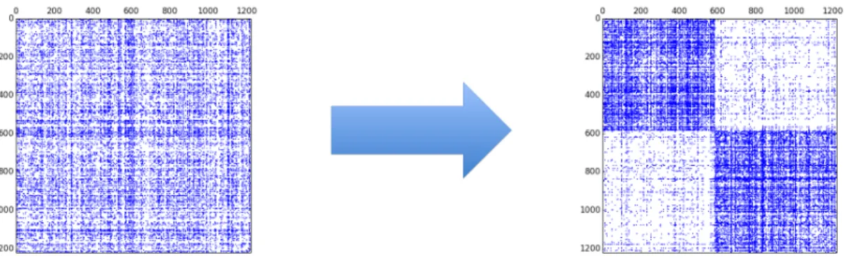
Figure 1.3: Political Blogs data: Nodes grouped according to communities detected

to the rest of the graph, i.e., the probability of having an edge between two vertices belonging to the same group is higher than that of having an edge between vertices belonging to different communities. Consequently we would observe the number of intra community edges to be higher than inter community edges. The problem of community detection is to identify such groups or modules among the nodes such that when the nodes are ordered by their groups the adjacency matrix takes a block diagonal matrix as in Figure1.3.

Many researchers have proposed methods and algorithms for community detection in networks. Such methods can broadly be divided into three categories: methods based on probabilistic models, methods based on the maximization of a global objective function and those based on spectral or matrix factorization of the adjacency matrix or the Laplacian matrix. The stochastic blockmodel [71,118] is a statistical model for random graphs with a natural community structure. It is one of a large class of statistical models described in the literature for community detection in complex networks, which includes the latent variable [68] and latent space models [70], the degree corrected blockmodel [79, 186] and the mixed membership blockmodel [3]. Various likelihood maximization based inference strategies have been proposed in the literature to simultaneously infer the block assignments and the parameters in the stochastic blockmodel, e.g., profile likelihood maximization [17], maximizing the conditional likelihood [31], and variational EM under mixture model settings [37]. Other strategies involve Bayesian inference using Gibbs sampling or variational methods [89] and optimizing a modularity function over all possible partitions of the graph [113]. See [61] for a detailed review of statistical inference in networks.

communities and the degree density of networks for the estimation strategies to be consistent. [17] and [186] studied the conditions for community detection through modularity maximization under the stochastic blockmodel and the degree corrected stochastic blockmodel respectively. [31] laid down the conditions necessary for the consistency of maximum likelihood estimation under the stochastic blockmodel. This work was extended by [136] with a regularized estimator to high dimensional settings where the number of communities grows roughly as fast as the number of nodes. [26] derived consistency and [18] derived asymptotic normality of the maximum likelihood estimators and their variational approximations in the mixture model settings. Spectral clustering at its variants have also been studied extensively by several authors [135,130,76,93] under both stochastic blockmodel and degree corrected stochastic blockmodel.

Although the problem of detecting modules or communities is relatively well studied for single layer networks [51], the same problem for multi-layer networks has not been studied well in the literature until recently. Our objective in this dissertation is to develop methods for community detection in both uni-layer and multi-layer networks. For multi-layer networks we wish to develop methods that can take into account the information present in all the network layers simultaneously. Recently there has been a surge in analysis of networks with multiple layers [13, 11, 82]. For community detection in multi-layer networks, we consider a natural extension of the standard stochastic blockmodel to multi-layer settings that we will call “multi-layer stochastic blockmodel” (MLSBM). This model, also considered in [67] as “graph SBM”, is in the spirit of multi-relational models described in [71], [156] and [80]. [67] proved the consistency of the maximum likelihood estimates in this model when the number of relations grows. They keep the number of nodes (and hence the number of communities) fixed. However, as we will see later in both the asymptotic analysis and simulation studies that MLE in this model does not perform very well when either the number of communities grows fast or the network layers are sparse on average. Hence, we propose a restricted version of this model through restrictions on the parameter space which is capable of handling networks with a large number of communities. We call this model “restricted multi-layer stochastic blockmodel” (RMLSBM).

We derive conditions on the growth of the number of communities and the average edge density of the networks under which the maximum likelihood estimate of the class assignment vector is

consistent (in the sense that the proportion of misclassified nodes tends to 0 as the number of nodes, and possibly the number of relations as well, grows). We further derive the minimax rates of error for community detection in MLSBM and obtain thresholds for consistent community detection. To compute the unknown class assignments and block model parameters simultaneously, we follow [37] and propose a variational estimation strategy.

A few modularity measures have also been proposed in the literature. [111] used a null model formulated in terms of stability of communities under Laplacian dynamics in networks to derive a modularity measure for multi-layer networks with inter-layer node coupling. Another extension of the Newman-Girvan modularity to multi-layer settings as a sum of layer-wise modularities was mentioned by [11,139]. Aggregation of adjacency matrix as a way of combining information from multiple graphs has also been explored in the literature. However, community detection on such aggregated graph does not always perform quite well as the different types of layers might have quite different properties and signal quality which will get lost due to aggregation.

In this dissertation we take two principled null model based approaches to derive modularity measures. Our first family of modularity measures are based on the difference between the observed and the expected intra-community edges under a specified null model in the network, while the second family of modularities are based on maximized likelihood inference of probabilistic random graph models with community structure. The second family can also be viewed as a “difference” between observed and expected structure of the network in terms of both inter and intra community edges, however the difference in this case will be expressed in terms of Kullback-Leibler divergence. Turning our attention to uni-layer networks we consider methods for community detection in networks based on the non-negative matrix factorization of the Laplacian matrix of the net-work. Non-negative matrix factorization (NMF) has received considerable attention in the machine learning and data mining literature since it was first introduced in [91]. The method has many good properties in terms of performance and interpretability, and is extremely popular in many applications including image and signal processing, information retrieval, document clustering, neuroscience and bio-informatics. A matrixX is said to be negative if all its elements are non-negative, i.e., Xij ≥0 for alli, j. The general NMF of orderK decomposes a non-negative matrix

When K ≤ min{M, N}, NMF can also be looked upon as a dimension reduction technique that “decomposes a matrix into parts” that generate it [91].

NMF has also been applied in the context of clustering [178, 43, 42, 81]. The “low-rank” NMF, where K ≤ min{M, N}, can be used to obtain a low-dimensional factor matrix, which can subsequently be used for clustering. [43] showed interesting connections of NMF with other clustering algorithms such as kernel k-means and spectral clustering. For applications in graph clustering where we generally have a symmetric adjacency matrix or a Laplacian matrix as the non-negative matrix, a symmetric version of the factorization was proposed in [170]. This factorization, called the symmetric non-negative matrix factorization (SNMF), has been empirically shown to yield good results in various clustering scenarios, including community detection in networks [170, 86]. [7] used a special case of SNMF, the left stochastic matrix factorization, for clustering, and derived perturbation bounds. [180] used a regularized version of the SNMF algorithm for clustering, while [129] used a Bayesian NMF for overlapping community detection. In this dissertation we consider another non-negative matrix factorization designed to factorize symmetric matrices, the orthogonal symmetric non-negative matrix (tri) factorization (OSNTF) [42,127].

We use the normalized graph Laplacian matrix as our non-negative matrix for factorization instead of the usual adjacency matrix, as it has been recently shown to provide better clustering quality in spectral clustering for graphs generated from the SBM [138]. In contrast with earlier approaches, the requirement of being orthogonal in OSNTF adds another layer of extra constraints, but generates sparse factors which are good for clustering. It also performs well in our experiments. We prove that OSNTF is consistent under both the stochastic block model and its degree corrected variant. Through simulations and real data examples we demonstrate the efficacy of both OSNTF and SNMF in community detection. In particular we show the advantages of proposed methods over the usual Laplacian based spectral clustering and its modifications in terms of regularization and projection within unit circle [93, 130]. The proposed methods do not require such modifications even when there is high degree heterogeneity in a sparse graph. An application to the widely analyzed political blogs data [2] results in a performance superior to the state of the art methods like SCORE [76].

detection in multi-layer network clustering. The problem is also related to a more general class of problems that generally goes under the theme of multi-view clustering and has received considerable attention over the last decade, particularly in the computer science community. Numerous methods have been proposed to combine information from multiple views of a multi-view relational data for clustering. The goal is usually to leverage the diversity and often complimentary nature of the information in different layers to outperform simply summing the layers or using any one of the layers [96]. A great many of those methods use spectral clustering or a low rank matrix factorization as a basis [99,187,143,155,88,116,45,96].

The “linked matrix factorization” algorithm in [155] and “RESCAL” algorithm in [116] ap-proximate the adjacency matrices in each layer of a multi-layer graph, or each slice of a three way tensor, with a low rank symmetric matrix factorization. While one of the factors is shared the other one varies across layers or slices. Although the algorithms employed in the two papers are quite different, the factorization in both cases is computed by minimizing an identical joint Frobe-nius norm objective function. [45] used similar common low rank matrix factorization ideas with a slightly different objective function to obtain a “joint spectrum” of a multi-layer graph which is subsequently used for clustering.

The co-regularized spectral clustering in [88] with centroid based co-regularization maximizes the combined normalized cut objective function over the Laplacian matrices from all views of the data, subject to a smoothness penalty. This idea is similar to the evolutionary spectral clustering used in [30] for clustering dynamic networks with a temporal smoothness penalty, and is part of a general theme of co-regularization in multi-view machine learning [177]. The co-regularization framework was extended to “joint non-negative matrix factorization” using a Frobenius norm based objective function in [96]. See [151] and [177] for surveys of multi-view learning methods.

However, there is a lack of theoretical understanding of the objective functions in these spectral and matrix factorization based methods. Researchers often rely on simulations and applications to specific datasets to compare the methods. However, this approach fails to explore different scenarios that might arise in practice. For example, in multi-layer network applications, the component layers might have very different sparsity, signal quality and node degree distributions. Hence it is important to explore the utility of the methods under different statistical models and asymptotic

Figure 1.4: Mean community structure in the functional network of brain regions in a group of 70 healthy subjects. Nodes : Regions of interest from AAL atlas, colored by communities. Edges : Mean functional connectivity.

settings through a principled theoretical study. In Chapter 5 we analyze a number of such methods under the MLSBM.

1.3

Groups of networks in neuroimaging studies

A relatively new but rapidly growing application area of network science is neuroimaging, where it is used in the analysis of anatomical and functional connectivity among the brain regions (See [137,25,74,146] for reviews). In network neuroscience a typical approach is to construct functional brain networks based on measures of inter-regional associations obtained from various sources of measurements including the functional magnetic resonance imaging (fMRI) with blood oxigen level dependent (BOLD) signals [12,141]. Modern neuroimaging experiments typically involve multiple subjects and multiple trials across the subjects. Various properties of the functional network (e.g., community structure, modularity, resilience, connectivity, degree) is then investigated and contrasted among the subjects or groups of subjects [25,162]. The inter-subject and inter-group variations in many such network metrics have been related to cognitive ability and diseases in the literature [12,149,74,77,171,23,182,101,4].

and responses to changing environmental conditions other than the experimental condition, the measured networks vary from subject to subject. Consequently the community structure obtained also significantly varies from subject to subject within a group of subjects or even from trial to trial within a subject [149, 142, 110, 173, 16]. In the neuroimaging studies the researchers are typically interested in inference about the two populations and the subjects in the two groups serve as random samples from the two populations. Hence to facilitate comparison across groups of populations it is important to build statistical models for a random sample of networks from a population of networks so that we can quantify the uncertainty in the inference from the present sample. The issue of consistency of network modules across different networks both at module level and at node level is investigated in [148]. A number of researchers has also investigated the consistency of brain modules across subjects and population differences from two groups of subjects [110,4,54].

Unfortunately most of the literature on networks deal with a single instance of a network. This is primarily due to the fact that network data collection usually involves observing a network at one time point or tracking its evolution over time. However modern application of networks in neuroscience brings in a unique challenge and opportunity in terms of multiple instances of interactions among the same set of nodes. The central question we investigate is how to quantify the uncertainty in community structure due to subject specific variations within a group of subjects which can be thought of as a sample from a population, so that two groups (populations) of subjects can be statistically compared. Our approach is to develop methodology in spirit of random effects linear models. The challenge is to characterize variations in a sample from the population which will then help us separate systematic variations from variations due to sampling noise.

The rest of the dissertation is organized as follows. Chapter 2 first extends stochastic blockmodel to multi-layer settings and defines MLSBM and RMLSBM and then investigates the asymptotic consistency of MLE of those models along with properties of the models in terms of minimax rates and sharp thresholds. Chapter 3 defines a number of null models for multi-layer networks and derives various modularity measures for community detection based on those null models. Chapter 4 focuses on community detection in uni-layer networks using NMF based methods and analyzes the theoretical properties of the method. Chapter 5 theoretically analyzes the spectral and matrix

factorization based optimization methods for multi-layer community detection. Finally in Chapter 6 we develop models and methods for joint community detection in a group of related networks.

Chapter 2

Community detection in multi-layer

networks through multi-layer

stochastic blockmodel

This chapter is organized as follows.1 Section 2.1 extends the stochastic blockmodel to multi-layer settings and defines the two models, MLSBM and RMLSBM. Section 2.2 settles the consistency of the community assignments through maximum likelihood estimation in the two models when the true data generating model is MLSBM. Section 2.3 describes two estimation strategies for the MLEs in the two models. Section 2.4 describes a few baseline procedures and Section 2.5 compares the multi-layer models with the baseline models in terms of minimax error rate and sharp threshold results. Section 2.6 describes the results of a simulation study to validate the theoretical results. Section 2.7 presents the application of the methods to the Twitter UK politics data set. Section 2.8 gives concluding remarks.

2.1

Extension of blockmodels to multi-layer settings

We consider an undirected multi-layer graph G = {V, E}, where the vertex set V consists of N

vertices and the edge set E consists of edges ofM different types representing different relations. We can view the multi-graph as a graph with vector valued edge information, i.e., the adjacency matrix A consists of elements Aij, who are themselves M dimensional vectors: Aij ={A(1)ij , A

(2) ij ,

. . . , A(M_ij )}. An alternative way to approach the problem is to view the multi-graph as a collection ofM,N×N adjacency matrices{A(1), A(2), . . . , A(M)}, each corresponding to one particular type of relation. The rest of the set up is similar to the regular stochastic block model (SBM) for one-layer case with K blocks [118]. We assume the number of communities K is known. Let

z = {z1, z2, . . . , zN} be the community indicator vector for the N nodes, such that each zi takes

1_{This chapter is based on research published as: S. Paul and Y. Chen. Consistent community detection}

in multi-relational data through restricted multi-layer stochastic blockmodel. Electronic Journal of Statistics,

exactly one value from the set{1, . . . , K}and zi =q if and only if nodeibelongs to communityq.

Conditional on the community indicator vectorz, the edges are formed independently as Bernoulli random variables with probabilities depending only on the community assignments and the type of edges. In what follows we describe the two extensions of the standard SBM to multi-layer settings. Except for the estimation algorithm, the model is always represented as a conditional block model andz is assumed to be a fixed unknown parameter of the model and needs to be estimated from data. Conditioned on the community assignments of the nodesziandzj, the edges are formed

independently following Bernoulli distribution

A(m)_ij |(zi =q, zj =l)∼Bernoulli(P_ql(m)).

The first model assigns a separate probability for themth type of edge between nodes belonging to the qth and the lth community independent of all other edges. We call this model the “multi-layer stochastic blockmodel” (MLSBM). The probability of anmth type of edge between nodes i

and j belonging to communitiesq and l respectively can be written as

P_ij(m) =π_z(m)_izj =π_ql(m), i, j∈ {1, . . . , N}, m∈ {1, . . . , M}, q, l∈ {1, . . . , K}.

The set of parameters for the model, π = {π_ql(m); q ≤ l, q, l ∈ {1, . . . , K}, m ∈ {1, . . . , M}} has

K(K+ 1)M/2 elements. This model is “saturated” in the sense that we have a different parameter for each of the different types of edges between nodes belonging to different communities. Denote the range of this parameter set or array as Π ={π ∈[0,1]K(K+1)M/2_}.

In our asymptotic settings, where both N and M grow and K grows with N, the number of parameters to be estimated in the MLSBM grows as K2M and quickly becomes large. Hence the MLE performs poorly especially when the individual network layers are sparse. This problem does not arise in the asymptotic settings of [67] where onlyM grows and N, K remain fixed. However, it has been empirically shown that in most real world networks the average cluster size does not grow with the size of the network [94,136,19] and consequently, K grows with N. Hence in our asymptotic settings where N grows, keeping K fixed would be rather unrealistic. This motivates us to propose the second related model whose number of parameters grows much slowly compared

to MLSBM.

The second model assumes the probability of the mth type of edge appearing between nodes

i and j is governed by two factors: the first one being the community assignment of the two nodes and the second one being the type of edge. Hence the model has two sets of parameters: a

K×K parameter matrix πK×K corresponding to the community structure, and anM ×1 vector

βM×1 which contains the parameters for different types of edges. We call this model the restricted

multi-layer stochastic blockmodel (RMLSBM).

Notice that in the second model, if the edges were all of the same type, we would just have

βm =β for all m∈ {1, . . . , M}and then we will recover the standard stochastic blockmodel, with

probabilities of edges determined solely by the community assignments. On the other hand, if we did not have a community structure, but M types of edges, then πql would be identical for all

communities q, l and the probability of an edge between nodes i and j will solely be determined by the type of edge. This model can retrieve information from sparse but highly informative edge types as the sparsity of the network layers will be captured in theβm parameters. Hence, although

we assume the edges to be conditionally independent, this model induces two types of correlations unconditionally — among the edges of the same type and among the edges that share nodes of the same community.

The probability P_ij(m) in RMLSBM , which denotes the probability of an mth type of edge between nodes i and j belonging to communities q and l respectively, can be modeled in the following way with the logit link function

logit(P_ij(m)) =πql+βm, i, j ∈ {1, . . . , N}, m∈ {1, . . . , M}, q, l∈ {1, . . . , K}.

This model hasK(K+ 1)/2 +M parameters for an undirected graph. Hence, when bothK andM

grow, the growth rate in the number of parameters for this model is the same as the maximum of the growth rates inK2 and M. In comparison, the number of parameters in MLSBM would grow asK2_{M. This makes the maximum likelihood estimator in RMLSBM a regularized estimator.}

For the RMLSBM to be identifiable, we require the parameters βm to satisfy the condition P

mβm = 0. Hence we have one less free parameter. Denote the set of parameters for RMLSBM

RK(K+1)/2+M_, P

mβm = 0}. To prove the consistency of maximum likelihood estimation under

MLSBM, we assume πql, βm ∈ (−Clog(M N2), Clog(M N2)) for some constant C > 0. This

condition ensures that πql and βm are bounded away from ±∞.

2.2

Consistency

In this section, we discuss the consistency of maximum likelihood estimation of the proposed models under three asymptotic regimes with varying conditions imposed on the growth of the number of communities (K) and the expected total number of edges of the multi-layer graph (L). We first define a one to one transformation of the parameters of RMLSBM as

φ(m)_ql = logit−1(πql+βm) =

exp(πql+βm)

1 + exp(πql+βm)

. (2.2.1)

Now we assume that the data are generated from the more general model MLSBM and view RMLSBM as a MLSBM with the following restrictions on the parameters:

Φ ={φ∈[0,1]K(K+1)M/2 : φ(m)_ql = logit−1(πql+βm), (2.2.2)

πql, βm ∈(−Clog(M N2), Clog(M N2))}.

This way the MLE in RMLSBM can be thought of as a restricted MLE (RMLE) of MLSBM. Our aim is to investigate the consistency of both the MLE and the RMLE under three asymp-totic regimes where we let either the number of nodes (N) or the number of types of edges (M) or both to grow. This setup is quite appropriate for modern day multi-layer networks, where data collection increases both in terms of new entities as well as new features or layers getting added to the database. Consequently methods are being sought which would be consistent in such situations. Some consistency results for the MLE were obtained in [67] under the settings whenM grows, but

N and consequentlyK remain fixed. Here we prove consistency results for the MLE in the more general asymptotic setting where N can also grow (and K grows with N). We then compare the MLE with the restricted estimator in terms of the sufficient asymptotic conditions for consistency. The different asymptotic setups we consider under the three regimes of growth in N and M are

described below.

1. As bothM and N grow, letK =O(N1/2_{) andL=ω(M N(logN)}3+δ_{) for some δ >0 for the}

MLE, while K = O((M N)1/2−) and L = ω(M N(logN)3+δ) with , δ > 0 for the RMLE. For the RMLE, we further require that M =O(N) so that K does not exceedN.

2. As N grows, M either is fixed or grows slower than N, i.e., either M is O(1), or M → ∞ and M = O(N). In this regime, let K =O(N1/2_{), L =ω(N(logN)}3+δ_{) for someδ > 0 for}

the RMLE.

3. As both N → ∞ and M → ∞ with M growing faster thanN, i.e., M = ω(N), for RMLE we consider two related setups: (a) K = O(_logMN_logN), L = ω(M N(logN)1+δ) for some

δ > 0; and (b) K = O(N1/2_{), L is either ω(M(logM)}2+δ_(logN)1+δ_{) for some δ > 0 if}

(logM)2+δ = O(N), or ω(M N(logN)1+δ) for some δ > 0 otherwise. In setting (a), we further require logM to grow slower than N for the growth of K to be meaningful. Also, in that setup if logM grows at the same rate as (logN)β for some β > 0, the number of communities grows almost as fast as the number of nodes except for the log terms and is “highest dimensional” in the sense of [136].

Note that the first regime assumes no relation between the growth rates ofN andM, while the next two regimes assume certain relations between the two growth rates. So the last two regimes can be thought of as special cases of the first one in terms of the growth rates of N and M. Naturally we expect some relaxation in the required growth conditions onK andLin the last two regimes. The asymptotic setups described above reflect this relaxation for the RMLE. However no such relaxation is possible for the MLE. Hence we will prove that MLE in MLSBM is consistent under the first asymptotic regime, whereas MLE in RMLSBM (i.e., the RMLE of MLSBM under the restrictions defined by Equation (2.2.2) is consistent under all three asymptotic regimes. We point out that the MLSBM, despite being intuitively the simplest extension, does not perform well for community detection in multi-relational networks if the networks are sparse at an average or contain a large number of communities. While the sufficient asymptotic conditions are not enough for a theoretical comparison between the methods, this observation is corroborated by an extensive simulation study comparing the two methods that mimics the asymptotic setup.

2.2.1 Preliminaries

Since in this chapter our primary interest is in modeling multi-layer networks where layers are sparse on an average, we require the true MLSBM model probabilities π_ql(m) to satisfy certain sparsity conditions. As [186] pointed out, if the block model probabilities remain fixed as N

increases, then the network will be unrealistically dense. In this connection it is worth noting that [144] let the probabilities remain fixed and as a result the networks considered there have linearly increasing average degree, while both [17] and [31] considered networks with poly-logarithmically increasing average degree and hence gradually decaying probabilities. Here to keep the network sparse, we scale down the block model probabilities accordingly asN increases.

We introduce a new notation L0 to denote the quantity inside the asymptotic notation ω in the growth rate of L under different asymptotic setups. As an example, consider the case when

L=ω(M N(logN)3+δ), thenL0 =M N(logN)3+δ. Hence L0 can be viewed as the minimum rate at which L is required to grow under a particular asymptotic setup. The blockmodel parameters are restricted to have an upper bound that decreases with increasing N except for a small finite set indexed by the triplet Q={q, l, m} such that the expected number of edges in the set|EQ|=

o

L0 log(M N2₎

. For the set Q we can have _{M N}1 2 ≤ π

(m)

ql ≤ 1− M N1 2. For all {q, l, m} ∈/ Q, the

parameters are restricted in the following way

π(m)_ql ∈ 1 M N2, C L0 M N2_(logMlogN)2+δ , (2.2.3)

for some δ > 0 and some constant C, so that the upper bound is determined by the expected density of the network. The exact upper bound is determined by L0 and consequently, by the growth rate ofL and varies under the different asymptotic assumptions.

For any arbitrary partition z of the entities in the graph, the log likelihood of the set of M

adjacency matricesA={A(1), . . . , A(M)} under the MLSBM with parameters π={π_ql(m)}is

l(A;z, π) = M X m=1 X i<j {A(m)_ij logπz(m)izj+ (1−A (m) ij )log (1−π (m) zizj)}. (2.2.4)

symmetric matrices in{0,1}N×N _{and [0,1]}K×K_{respectively. The Bernoulli parametersπ}(m)

zizj depend both on the class assignment z and the type of relation m. For a fixed class assignmentz, letNq

denote the number of nodes assigned to class q, andnql denote the maximum number of possible

edges between classes q and l. So we have nql =NqNl and nqq= N₂q

. For an arbitrary partition

z, the MLE of π(z) is ˆ π_(z)ql(m) = 1 nql X i<j A(m)_ij 1{zi =q, zj =l}, m= 1, . . . , M, q, l= 1, . . . , K, (2.2.5)

where 1{·}is the indicator function. Note that for a fixed partition z, the denominator nql in the

MLE ˆπ_(z)ql(m) is the same for all edge types m.

Now we define the expectation of ˆπ(z) as ¯π(z) and that of l(A;z, π) as ¯lP(z, π) under the

inde-pendent Bernoulli(P_ij(m)) model. Then we have

¯ π(m)_(z)ql= 1 nql X i<j P_ij(m)1{zi=q, zj =l}, m= 1, . . . , M, q, l= 1, . . . , K, (2.2.6) ¯ lP(z, π) = M X m=1 X i<j {P_ij(m)logπ(m)zizj + (1−P (m) ij )log (1−π (m) zizj)}. (2.2.7) Clearly for a given z, ˆπ(z) and ¯π(z) are the maximizers of the functions l(A;z, π) and ¯lP(z, π)

respectively, and we letl(A;z) and ¯lP(z) denote the corresponding maximum values.

We extend Lemma 1 of [31] to multi-layer settings as follows:

l(A;z)−¯lP(z) = X m X i<j ( A(m)_ij log πˆ (m) zizj ¯ πz(m)izj ! + (1−A(m)_ij ) log 1−ˆπ (m) zizj 1−¯πz(m)izj ! ) +X−E(X) =X m X q≤l nqlD(ˆπ_(z)ql(m) ||¯π_(z)ql(m)) +X−E(X), (2.2.8) where X= M X m=1 X i<j A(m)_ij log ¯π (m) zizj 1−¯πz(m)izj ! . (2.2.9)

pa-rameters a and b respectively. This equation decomposes the difference between the maximized likelihood and its expected value in terms of ˆπ(z) and ¯π(z) for a given class assignment vector z.

Next we turn our attention to RMLSBM. As mentioned before, we consider RMLSBM as a re-stricted version of MLSBM, and the MLE of RMLSBM can be viewed as a RMLE of MLSBM under the restrictions. Given a class assignment z, the RMLE ˆπ(m)Rzizj ={ˆπ(z)ql, βˆ(z)m} is the maximizer of lR(A;z, πR), the multi-layer block model log likelihood within the restricted parameter space. Substituting the estimated parameters in the likelihood function gives lR_{(A;z), the maximum of}

the likelihood function within the restricted parameter space. However, no closed form solution exists for the RMLE. Instead we have the following M+K(K+ 1)/2 estimating equations:

∂ ∂βm :=X i<j A(m)_ij − exp(ˆπzizj+ ˆβm) 1 + exp(ˆπzizj+ ˆβm) ! , (2.2.10) ∂ ∂πzizj :=X i<j X m A(m)_ij − exp(ˆπzizj+ ˆβm) 1 + exp(ˆπzizj+ ˆβm) ! . (2.2.11)

One of the equations is redundant since if we add the equations in (2.2.10), the resulting equation is identical to the sum of the equations in (2.2.11).

Now we use the transformation defined by φ in Equation (2.2.1). The likelihood with respect to the new parameters can be represented as

lR(A;z, φ) = M X m=1 X i<j {A(m)_ij log φ(m)zizj+ (1−A (m) ij )log (1−φ (m) zizj)}, (2.2.12)

and the estimating equations in (2.2.10) and (2.2.11) can be written as 1 N(N + 1)/2 X q≤l nqlφˆ(m)_(z)ql= 1 N(N + 1)/2 X q≤l X i<j A(m)_ij 1{zi =q, zj =l} = 1 N(N + 1)/2 X i<j A(m)_ij , m= 1, . . . , M, (2.2.13) 1 M X m ˆ φ(m)_(z)ql= 1 M nql X m X i<j A(m)_ij 1{zi=q, zj =l}, q≤l∈ {1, . . . , K}. (2.2.14)

model. Hence we haveK(K+ 1)/2 +M−1 independent equations which will together determine the MLE of K(K+ 1)/2 +M −1 free parameters in the set π_(z)R . Here it is understood that the estimation procedure ensures that the finiteness condition of πql and βm are respected possibly by

restricting πql, βm ∈ (−Clog(M N2), Clog(M N2)). By the functional invariance property of the

MLE, ˆφ(m)_(z)ql= exp(ˆπql+ ˆβm)

1+exp(ˆπql+ ˆβm) is the MLE ofφ

(m)

(z)ql. Note that the minimum value any ˆφ (m)

(z)qlcan take

due to the imposed boundedness constraint is 1/M N2. This value is sufficiently small so that none of the partial sums in the left hand side of Equations (2.2.13) and (2.2.14) exceeds 1.

As before we define expectations of ˆφz as ¯φz and that of lR(A;z, φ) as ¯lRP(z, φ) under the

independent Bernoulli(P_ij(m)) model. Then,

¯ lR_P(z, φ) = M X m=1 X i<j {P_ij(m)log( ¯φ(m)_zizj) + (1−P_ij(m)) log(1−φ¯(m)_zizj)}. (2.2.15)

For a given class assignment z, ˆφz and ¯φz are the maximizers of the functions lR(A;z, φ) and

¯

lR_P(z, φ) respectively, and we letlR(A;z) and ¯lR_P(z) denote the corresponding maximum values. The difference between the maximized values of the observed and expected likelihood can be decomposed in two parts similar to Equation (2.2.8) as follows

lR(A;z)−¯lR_P(z) =X m X q≤l nqlD ˆ φ(m)_(z)ql || φ¯(m)_(z)ql+X−E(X), (2.2.16) where as before, X= M X m=1 X i<j A(m)_ij log ¯ φ(m)zizj 1−φ¯(m)zizj ! . (2.2.17)

A proof of this result can be found in Section 2.10. Since the maximum of unrestricted likelihood would be at least as large as the maximum of restricted likelihood, we havel(A;z)≥lR(A;z) and ¯

lP(z)≥¯lPR(z) for allz.

Now let ¯zdenote the true partition. Further let ˆzand ˆzR _{denote the MLEs of ¯zunder the two}

models MLSBM and RMLSBM respectively, i.e.,

ˆ

z= arg max

ˆ

zR= arg max

z l

R_{(A, z). (2.2.19)}

2.2.2 Main results

We give several theorems in this section as we develop towards our main result. These theorems provide insights into the conditions required under the three asymptotic regimes discussed in the beginning of Section 2.2, which in turn provide comparison between the asymptotic behavior of MLEs in the two models MLSBM and RMLSBM. All the proofs are given in Section2.10.

The first three theorems bound the difference in the maximized log likelihood and its expected value for both MLSBM and RMLSBM as defined in Equations (2.2.8) and (2.2.16).

Theorem 1. Suppose a MLSBM and a RMLSBM, both with K classes and M layers, are fit-ted to the graph with adjacency matrix {Aij}i<j = {A(1)ij , . . . , A

(M)

ij }i<j, i, j = 1, . . . , N, where

A(m)_ij are independent Bernoulli(P_ij(m)) trials. For any class assignment z, suppose the estimate

ˆ

π_(z) = {ˆπ_(z)ql(m); q, l ∈ {1, . . . , K}, m ∈ {1, . . . , M}} maximizes the multi-layer block model likeli-hood l(A;z, π) and the estimate πˆR_(z) ={(ˆπ(z)ql,βˆ(z)m); q ≤l, q, l∈ {1, . . . , K}, m∈ {1, . . . , M}}

maximizes the likelihood from the model with the restricted parameter space defined by ΠR. Let

ˆ φ(z) = {φˆ (m) (z)ql; q, l ∈ {1, . . . , K}, m ∈ {1, . . . , M}} be defined from πˆ R (z) according to Equation

(2.2.1). Then for any >0,

P  max z X q≤l nql X m Dπˆ(m)_(z)ql || ¯π(m)_(z)ql≥   (2.2.20) ≤exp NlogK+M(K2+K) log N K + 1 − , P max z ( X m N(N + 1) 2 D   P q≤lnqlφˆ (m) (z)ql N(N + 1)/2 P q≤lnqlφ¯ (m) (z)ql N(N + 1)/2   ) ≥ ! (2.2.21)

≤exp NlogK+ (K2+K) log N M

1/2 K + 1 ! +Mlog N(N+ 1) 2 + 1 − ! , P max z ( X q≤l M nqlD 1 M X m ˆ φ(m)_ql 1 M X m ¯ φ(m)_ql ! ) ≥ ! (2.2.22)

≤exp NlogK+ (K2+K) log N M 1/2 K + 1 ! +Mlog N(N+ 1) 2 + 1 − ! .

The first result (2.2.20) provides a bound for the first part of the right hand side of Equation (2.2.8) for MLSBM. The results (2.2.21) and (2.2.22) provide a bound that will be used in Theorem 3to bound the first part of the corresponding likelihood decomposition for RMLSBM in Equation (2.2.16). In the proofs of the next two theorems, we first bound the second part of Equations (2.2.8) and (2.2.16), and then combine the results to provide a bound for the difference between the log likelihood and its expected value under any arbitrary partitionzfor MLSBM and RMLSBM respectively.

Theorem 2. Suppose a MLSBM with K classes and M layers is fitted to the graph whose edges A(m)_ij are independent Bernoulli(P_ij(m)) trials. If we further assume that (i) _{M N}1 2 ≤P

(m)

ij ≤1−M N1 2

for alli < j, (ii) K=O(N1/2), and (iii) the total expected number of edges of the entire multi-layer graph L=P