Sensorless Force Estimation for Robots with Friction

Sensorless Force Estimation for Robots with Friction

John W.L Simpson, Chris D Cook, Zheng Li

School of Electrical, Computer and Telecommunications Engineering

University of Wollongong

N.S.W 2522

[email protected]

Abstract

This paper describes a method for estimating forces applied at the end effector of a robot without the need for force sensors. Servo motor currents and positions are used together with an accurate system model to estimate applied forces. The system model includes inertia, friction and position dependent force components. The signal processing techniques required to extract the force information from the servo motor data are detailed and experimental results from a SCARA robot presented.

1 Introduction

Force control has been used in many robotic applications including assembly tasks, searching and grasping tasks and machining tasks such as grinding, and deburring. Typically these applications have been implemented using a force sensor to give a force feedback signal. In this paper a method to calculate forces applied by an end effector without the use of a force sensor is given. The method uses an accurate model of the robotic system plus servo motor position and current data to estimate the applied force.

Force sensors have a monetary cost and are typically less mechanically robust than the robots they are mounted on. In addition force sensors normally have as part of their design an elastic sensing element whose deformation is a measure of the applied force. This elastic element reduces the stiffness of the robot’s mechanical system. As a force is applied this leads to greater deflection of the end effector and greater positional error.

In robotic systems servo motor position and torque information (deduced from motor currents) has been used to calculate and control forces at a robot’s end effector This area of work is often referred to as implicit force control. The problem is that the motor’s torque has to overcome friction and other torques in addition to an often very small component related to the force or torque at the end effector. In addition, motor currents are notoriously

noisy with unwanted signals from a variety of motor and inverter related effects. [Gorinevsky et al, 1997] in their discussion of implicit force control schemes suggest that these can only be used with direct drive manipulator arms or if the friction in the gear trains is small. [Wada et al 1994] and [Rocco et al 1997] implemented force control schemes using a direct drive system. In this work models of the robotic manipulator have included inertia and viscous friction components. [Ohishi 1993] also used a direct drive mechanism including inertia viscous and coulomb friction in a force observer.

[Gorinevsky et al, 1997] also commented that in “most industrial manipulator systems joint friction by far exceeds the torques generated in contact tasks”. Other authors [Elosegui et al 1990], [Taghirad and Belanger 1997], [Taghirad et al ,1997], [Luh et al 1983] have used joint torque sensors to eliminate the effects of friction. The joint torque sensors are installed on the robot linkage side of the gear train and are used as a feedback signal in a torque control loop. [Elosegui et al 1990] details the use of joint torque sensors to reduce the effects of the non-ideal transmission due to the presence of stiction, coulomb friction and cogging. Joint torque sensors have been found effective in force control loops as have the use of force sensors at the end effector. However all these schemes have the disadvantage of having to use additional sensors. The force estimation techniques described in this paper are capable of dealing with non-ideal transmission, friction and motor cogging and other effects without the need for additional force sensors since they require measurement only of motor current.

The servo motor moving each axis of a robot is typically supplied by electronic servo drives operating in current control mode. The servo drive applies a known current to the servo motor and using the motor's torque constant the motor torque can be calculated. In the work presented here the motor torque is assumed to be made up of the torque accelerating the mechanical components, the torque to overcome friction, the torque required to overcome a number of position dependent torques caused by the drive train and servo motor construction and the torque derived

Proc. 2002 Australasian Conference on Robotics and Automation Auckland, 27-29 November 2002

from the end effector’s operation.

The mechanical system used in the SCARA robot considered here has a gearbox between the servo motor and the robot’s links. The force applied at the end effector will be significantly reduced by the gearing ratio (at least 1:80 for this robot) and so will typically be a very small part of the total servo motor torque. To be able to separate the torque component due to the applied force from the other motor torques an accurate system model is needed. This includes the inertia, viscous and coulomb friction, and position dependent torque components. Other authors [Webb et al, 1998], [Popovic et al, 1998] and [Armstrong 1991] have document position dependent components in complex mechanisms. It is shown here that many torque components in the motor currents are position dependent, and that they can be removed by appropriate signal processing, thus allowing a substantial improvement in the accuracy of estimating end effector forces from motor currents.

2

Experimental Setup

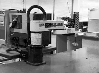
The force estimation techniques were implemented on a Hirata ARI350 SCARA Robot. The robot has 4 axes. The main rotation axes, A and B, have harmonic gear arrangements. The gearing ratios are 100 and 80 for the A and B axes respectively. The linear Z-axis has a belt and screw arrangement and the wrist rotation W-axis is a belt and gear arrangement. DC motors power all the axes. The A and B axis motors are driven by Baldor TSD series DC servo-drives and the Z and W axes are driven by Yaskawa DC servo-drives. All the servo drives are current controlled. The robot controller has been rebuilt to be completely controlled by a dedicated Digital Signal Processor (DSP). The Robot and its control cubicle are shown in figure 1

Figure 1 SCARA Robot and Control cubicle

The DSP reads all the shaft encoder position data and end travel limit switch information, implements the control strategy and outputs the drive signal. The DSP system gives a flexible and easy to program system, and very fast sample rates, and enables the easy implementation of a variety of control and signal processing strategies.

An external force is applied to the end effector of the robot by stretching a spring. One end of the spring is connected to a fixed point and the other end is connected to the robot’s end effector. In the experiments, coordinated motion of the A and B axes of the Hirata robot is used to track a circular path about a fixed point. For this arrangement the magnitude of force will be constant and the direction of the force will always be in adirection normal to the circular path being tracked.

The magnitude of the spring force can be changed by tracking circular paths of different radii. A schematic representation of the Hirata robot’s path and the spring arrangement is shown in figure 2.

Figure 2 Friction Controller Block Diagram

The link lengths of the A and B axes are denoted as ra and

rb and are also shown in figure 2. Let the magnitude of the force applied by the spring be Fspring. Let θF be the angle the direction of the spring force makes with the x axis. The spring force can be resolved into its x and y components

Fx and Fy respectively such that:

F spring x F

F = cosθ Fy =FspringsinθF Eq 1 Let (x,y) be the Cartesian coordinates of the end effector’s position. The (x,y) coordinates are related to the A and B joint angles θa and θb respectively by the standard kinematic equation for a SCARA robot [Schilling, 1990]

x=racosθa+rbcos(θa+θb)

y=rasinθa+rbsin(θa+θb) Eq 2 The force Fspring. will produce torques at the A and B joints denoted Ta and Tb respectively. Letting a torque that causes rotation in the clockwise direction be positive the relationship between the spring force components and the joint torques is given by

:

The results given in this paper are for the robot tracking a circular path with a 130mm radius and an angular velocity

spring F x F y F a r b r X Y a θ b θ F θ Spring Robot Path F spring xFF=cosθ F spring yFF=sinθ

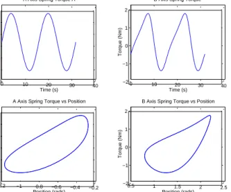
of 0.4rad/sThis corresponded to a spring force of 3.5 N which is only about 4% of the robot’s maximum force capability. Extracting such a small force from the motor currents hence represents a challenging test for the proposed method. Using Eq 1 and 3 the expected torques at the A and B axes joints can be calculated and are shown in figure 3

Figure 3 A and B Axes Torques

The top two graphs in this figure show the spring torque values plotted against time and the bottom two graphs show the torque values plotted against position. In section 4 the graphs plotting torque against position are used as a baseline to compare the output of each stage of the force estimation signal’s processing.

3

Position Dependent Torque Variations

Even though inspection of the motor currents in the time domain seem to show a massive amount of ’noise’, it turns out that viewed in the position domain the situation becomes more optimistic. Position dependent torque components can be considered as part of an accurate system model used to calculate end effector forces from servomotor current information. These components have been found to be due to a number of causes including motor poling, stator slot cogging, and various perturbations introduced by the mechanical drive train design, such as gear and belt teeth and shaft eccentricities. In addition there are a number of frictional torque components. In the rest of the discussion here all these components are referred to as Position Dependent Torque Variations (PDTV)

To discuss PDTV a number of terms need to be introduced. For a periodic function of angular position θ measured in radians let the period be Ρ. This will be referred to as the position period. The position frequency

Φ/ _{is the inverse of the position period. The units for the}

position frequency Φ/ are rads-1. A more convenient set of units is to relate position frequency to the revolutions of the servo motor. The units used here are Cycles Per Revolution (CPR) i.e. the number of times a particular

position frequency occurs per revolution. There is a gear box between the servo-motor and the robot linkage on each of the And B axes of the robot and the gear ratio is denoted as n. The relationship between the position frequency in rads-1Φ/, position frequency in CPR Φ, the gear ratio n and position period Ρ is given in Eq 4

Ρ =

Φ 1 Φ=2πΦ′ n Eq 4

A PDTV with a position frequency of 10 CPR occurs 10 times per revolution of the servo motor or 10n per revolution of the robot’s axis. The PDTV component will have a position period of 2π/10n rads.

To identify the PDTV, experiments are conducted where each robot’s axis is run at as slow a ’constant’ velocity as is practical with no end effector load. The digital control system has a set sampling rate and records the position and torque data at set time intervals. The position and torque values recorded at the same time are grouped together. Since the velocity will never be perfectly constant the torque values will not be recorded at equally spaced positions. To deal with this problem the position axis is divided up into a number of position intervals or position bins. If more than one torque value falls within each bin these values are averaged together to give a single torque value for the position bin. If at least one torque value falls within each position interval then the signal can be regarded as a “discrete position” signal. All the signal processing techniques that can be applied to a discrete time signal can then also be applied to this discrete position signal. Hence position sampling rates, Nyquist position frequencies and aliasing have to be considered for the discrete position signal as they would have to be considered for a discrete time signal.

Consider the differential equation describing the system with inertia J, viscous friction fv, Coulomb friction fc, PDTV Tpos(θ): ) ( 2 2 θ θ θ pos c v motor f T dt d f dt d J T = + + + Eq 5

The inertia, viscous and Coulomb friction parameters were measured directly and stored in a table, but the acceleration and velocity must be calculated from the position data. The PDTV signal is then the motor torque minus the torque accelerating the mechanism and the Coulomb and viscous friction torques.

The PDTV signal calculated at each time interval is turned into a discrete position signal and a Fast Fourier Transform (FFT) is applied to this signal. A typical resulting position frequency spectrum is shown in figure 4.

The PDTV magnitudes do change with velocity, and also over time as mechanical components wear, or change after maintenance, due to realignment of shafts, bearing preloads and so on. However the frequencies at which PDTV occur are highly repeatable and do not change with

0 10 20 30 40 −3 −2 −1 0 1 2 3

A Axis Spring Torque A

Time (s) Torque (Nm) 0 10 20 30 40 −2 −1 0 1 2

B Axis Spring Torque

Time (s) Torque (Nm) −1.2 −1 −0.8 −0.6 −0.4 −0.2 −3 −2 −1 0 1 2 3

A Axis Spring Torque vs Position

Position (rads) Torque (Nm) 0.5 1 1.5 2 2.5 −2 −1 0 1 2

B Axis Spring Torque vs Position

Position (rads)

Figure 4 B Axis PDTV Position Frequency Spectrum

velocity or over time. Hence for a given mechanism the position frequency spectrum only needs to be characterised once and only at one velocity.

4

Force Estimation Experiments

The estimation of external forces applied by the end effector requires an accurate model of the mechanical system, including its mass, friction and PDTV. When no external forces are applied the torque delivered by the motor to the system is assumed to accelerate the mechanism and to overcome its friction and PDTV. When an external force is applied the difference between the model and the observed motor torque is then the external applied force. The friction model includes Coulomb and viscous friction. The PDTV are implicitly included as part of the signal processing. In the experiments conducted here the differential equation describing the system is given by :

Tspring is the torque component due to the applied spring force Fspring. The Tspring component is either the torque component Ta or Tb as given by Eq 3 depending on whether the A or B axis is being analysed.

The B axis position affects the A axis inertia but apart from this the A and B axis are assumed to be independent of each other. Centripetal forces, Coriolis forces and coupling inertias have been neglected.

As the robot attempts to describe a circle at constant velocity for a given spring tension the motor torque Tmotor and position θ data are recorded. From the position data the velocity and acceleration values are calculated. Hence inertial torques can also be calculated. Estimates of the viscous and coulomb friction parameters are derived from previous experiments by direct measurement. Thus from the known data a torque estimation signal Test can be generated and is given by:

The torque estimation signal includes the spring torque component Tspring, the PDTV components Tpos(θ) and noise signal.

Test =Tspring +Tpos

( )

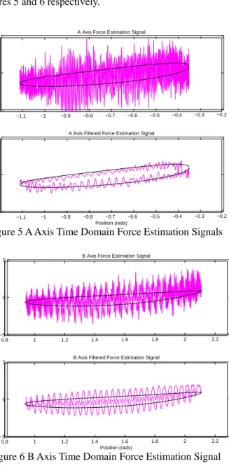
The signal processing aims to remove the noise and PDTV signals from the torque estimation signal to leave the spring torque. The torque estimation signals for the A and B axes of the Hirata robot are shown in the top plots of figures 5 and 6 respectively.

Figure 5 A Axis Time Domain Force Estimation Signals

Figure 6 B Axis Time Domain Force Estimation Signal

The lighter line plots show the force estimation signal calculated from the recorded position and torque data. The dark line is the torque value calculated from the applied spring force and is the same as that shown in figure 3. The first stage of the signal processing is to filter the force estimation signal with a low pass filter in the time domain. The filtered force estimation signals are shown in the bottom plots of figures 5 and 6. The low pass filter removes the higher frequency noise components which are mostly caused by decoder quantisation noise. This high frequency noise is made worse by the double

0 5 10 15 20 25 30 35 40 0 0.05 0.1 0.15 0.2 0.25 0.3 0.35 0.4 0.45 0.5 Position Frequency (CPR) T orq u e ( N m) ) ( 2 2 θ θ θ pos c v motor f T dt d f dt d J T = + + + c v motor est f dt d f dt d J T T = − θ₂ − θ − 2 −1.1 −1 −0.9 −0.8 −0.7 −0.6 −0.5 −0.4 −0.3 −0.2 −5 0

5 A Axis Force Estimation Signal

Torque (Nm)

−1.1 −1 −0.9 −0.8 −0.7 −0.6 −0.5 −0.4 −0.3 −0.2 −5

0

5 A Axis Filtered Force Estimation Signal

Position (rads) Torque (Nm) Eq 6 Eq 7 0.8 1 1.2 1.4 1.6 1.8 2 2.2 −5 0

5 B Axis Force Estimation Signal

Torque (Nm)

0.8 1 1.2 1.4 1.6 1.8 2 2.2 −5

0

5 B Axis Filtered Force Estimation Signal

Position (rads)

differentiation of the position data to calculate the acceleration value.

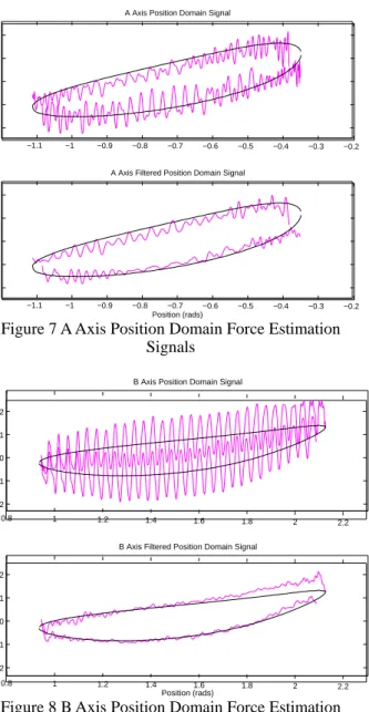
The filtered torque estimation signal is then turned into a discrete position signal. The position domain torque estimation signals for the A and B axes are shown in the top plots of figures 7 and 8

Figure 7 A Axis Position Domain Force Estimation Signals

Figure 8 B Axis Position Domain Force Estimation Signals

The next stage of the signal processing is to remove the PDTV components. The discrete position signal is processed with a filter with notches at the same position frequencies as the main PDTV components. For example these PDTV components are shown in figure 4 for the B axis.

The torque estimation signal after the PDTV components have been removed are shown in the bottom plots of figures 7 and 8. These show that the signal processing has significantly reduced the noise on the torque estimation signal for the A and B axes. The reduction in the noise was greater on the B axis than the A axis. Part of this was due

to the component of the force spring force seen at the B axes motor was a larger motor torque because the B axes has a lower gear ratio than the A axes. In addition the PDTV component were filtered more effectively on the B axes than the A axis. This was because the B axes had one large PDTV component at 2 CPR (as shown in figure 4) which is easy to filter. The A axis PDTV spectrum had more frequency components but of less magnitude and the position domain filtering wasn’t as effective.

5 Conclusions

External forces applied to the end effector of a robot will produce torques that the servo motors that drive each of the axes of the robot will have to overcome. The research presented here shows that these torques can be determined from servo motor current and position data in a SCARA robot whose mechanical system has a high gear ratio and in which friction is significant. The method uses a detailed model of the mechanical system and processing of the servo motor data in both the time and position domains.

The torque estimation technique was demonstrated for coordinated motion of two axes on a SCARA robot. Each axis moved with continually varying velocities to apply a constant but very small end effector force of only 3.5N. The method gave good estimates of force despite the demanding nature of this test.

Acknowledgements

This work was part of a project funded by the Australian Federal Government Cooperative Research Centre for Intelligent Manufacturing Systems and Technologies.

References

[Gorinevsky et al, 1997] Gorinevsky.D.M,

Formatsky.A.M, Schneider.A.Y, Force Control of

Robotics Systems, New York, CRC Press, 1997

[Wada et al 1994] Wada.H; Kosuge.K, Fukuda.T, Watanabe.K, “Design of force controller based on frequency characteristics,” IEEE International Conference on Robotics and Automation, Vol 1 pp

610-615, May 8, 1994

[Rocco et al 1997] Rocco P, Ferretti.G, Magnani.G, “Implicit force control for industrial robots in contact with stiff surfaces”, Automatica, Vol 33 No 11 pp2041-2047, 1997

[Ohishi 1993] Ohishi.K, “Sensorless force control using H acceleration controller,” Asia-Pacific Workshop on

Advances in Motion Control, pp13-16,15th June 1993 [Elosegui et al 1990] Elosegui.P, Daniel.R.W,

Sharkey.P.M, “Joint servoing for robust manipulators force control,” IEEE International Conference on

Robotics and Automation, Vol 1 pp 246-251, 13th May, 1990

[Taghirad and Belanger, 1997] Taghirad.H.D, Belanger.P.R, “Intelligent torque sensing and robust control of harmonic drive under free motion,” IEEE

International Conference on Robotics and Automation,

p1749-1754, April 1997 0.8 1 1.2 1.4 1.6 1.8 2 2.2 −2 −1 0 1 2 Torque (Nm)

B Axis Position Domain Signal

0.8 1 1.2 1.4 1.6 1.8 2 2.2 −2 −1 0 1 2 Position (rads) Torque (Nm)

B Axis Filtered Position Domain Signal

−1.1 −1 −0.9 −0.8 −0.7 −0.6 −0.5 −0.4 −0.3 −0.2 −2 −1 0 1 2 Torque (Nm)

A Axis Position Domain Signal

−1.1 −1 −0.9 −0.8 −0.7 −0.6 −0.5 −0.4 −0.3 −0.2 −2 −1 0 1 2

A Axis Filtered Position Domain Signal

Position (rads)

[Taghirad et al ,1997] Taghirad,H.D, Helmy.A, Belanger.P.R, “Intelligent built in torque sensor for harmonic drive systems,” IEEE Conference Instrument

and Measurement Technology., p969-974, May 1997

[Luh et al 1983] Luh.J.Y.S, Fisher.W.D, Paul.R.P.C, “Joint torque control by a direct feedback for industrial robots,” IEEE Transactions on Automatic Control, vol AC-28, No2, February, 1983

[Popovic et al,1998] Popovic, M.R, Goldenberg A.A, 1998 Modelling of Friction Using Spectral Analysis. IEEE Transactions on Robotics and Automation Vol 14/1:114-122.

[Webb et al, 1998] Webb, S, Cook , C.D 1998 Identification of Drive Train Torque Disturbances for an X-Y Table Test Bed, Proceedings of the Fifth International Conference on Control, Automation, Robotics and Vision, Singapore, Vol1: 439-443

[Armstrong 1991] Armstrong B, 1991 Control of machines with Friction MA Kluwer, Boston

[Schilling, 1990] Schilling R.J, “Fundamentals of

Robotics: Analysis and Control”, New Jersey,