SYBRAND JACOBUS MULLER
Thesis presented in fulfilment of the requirements for the degree of Master of Science in the Faculty of Science at Stellenbosch University.
Supervisor: Prof A Van Niekerk
DECLARATION
By submitting this thesis electronically, I declare that the entirety of the work contained therein is my own, original work, that I am the sole author thereof (save to the extent explicitly otherwise stated), that reproduction and publication thereof by Stellenbosch University will not infringe any third party rights and that I have not previously in its entirety or in part submitted it for obtaining any qualification.
With regard to Chapters 3 and 4 the nature and scope of my contribution were as follows:
Chapter Nature of contribution Extent of contribution (%)
Chapter 3
This chapter was published as a journal article (Muller & van Niekerk 2016a) and was co-authored by my supervisor who helped in the conceptualization and writing of the manuscript. I carried out the literature review, data collection and analysis components and produced the first draft of the manuscript.
SJ Muller 85% Prof A van Niekerk 15%
Chapter 4
This chapter was published as a journal article (Muller & Van Niekerk 2016b) and was co-authored by my supervisor who helped in the conceptualization and writing of the manuscript. I carried out the literature review, data collection and analysis components and produced the first draft of the manuscript.
SJ Muller 85% Prof A van Niekerk 15%
Date:
March 2017
Signature:
Copyright © 2017 Stellenbosch University All rights reserved
SUMMARY
Excessive accumulation of salt in the plant root zone has a deteriorating effect on vegetation growth, resulting in reduced crop yield and rendering fertile soil barren, and ultimately leads to decreasing food production. This problem motivates the critical need for active salinity monitoring, with an aim to implement rehabilitation and preventive measures. Conventional salinity monitoring methods, such as regular field visits and laboratory analyses of soil samples, are ineffective for frequent salt accumulation monitoring over large areas. Earth observation techniques can complement conventional methods and potentially improve the cost- and time-efficiency of the regular salt accumulation monitoring.
A review of literature identified a number of direct and indirect approaches for detecting accumulated salts using remote sensing. Given that salt accumulation in South Africa is most prevalent in irrigation schemes, the indirect approach, which mainly focusses on salt induced vegetation response, was identified as the preferred approach. Little is known about the optimal combinations of very high resolution satellite imagery and image classification techniques in South African irrigation schemes, where accumulated salt generally occurs in small localized patches. Consequently, two experiments were carried out to: identify suitable spectral and spatial resolutions of imagery; test the value of various image-derived features and classification techniques; and evaluate the spatial scale at which salt accumulation is best identified. The first experiment, applied on an agricultural field scale, analysed WorldView-2 imagery with statistical (regression) and machine learning (decision trees) techniques, and found clear relationships between salt accumulation and image transformations (vegetation indices and image texture). Spatial resolutions of six metres or higher were found to be most suitable. A higher spectral resolution marginally improved classification accuracies, but the increases were insignificant. The second experiment, applied on an irrigation scheme level, assessed SPOT-5 imagery with statistical (regression) and machine learning (various algorithms) techniques in two irrigation schemes. The failure to highlight any consistent image transformation or classification techniques for both irrigation schemes emphasised the negative effect of varying salinity tolerances of crop types and growing phases in identifying salt accumulation. Knowledge gained from the two experiments aided the development of a field level object-based monitoring system that showed sufficient transferability.
The quantitative experiments answered key research questions and will serve as a point of departure for future research regarding indirect methods for detecting salt accumulation in agricultural fields. This work will be instrumental in the establishment of a South African
salinity monitoring system – with the aim of rehabilitation – and will help to maximize agricultural production and ultimately contribute to sustainable food production.
KEYWORDS
Soil salinity, salt accumulation, irrigated agriculture, remote sensing, earth observation, regression analysis, decision tree analysis, supervised classification, machine learning, geographic object-based image analysis
OPSOMMING
’n Oormaat sout in ’n plant se wortelarea het ’n nadelige effek op die plant se groei, veroorsaak ’n afname in oesopbrengs en maak vrugbare grond onvrugbaar, wat uiteindelik tot ’n afname in voedselproduksie lei. Hierdie probleem motiveer die kritiese behoefte aan ’n stelsel wat grondversouting aktief moniteer, met die doel om versoute areas te rehabiliteer en te voorkom. Tradisionele metodes om grondversouting te moniteer sluit gereelde veldwerk en laboratoriumontleding van grondmonsters in, maar is nie vir die gereelde monitering van groot grondversoute-areas effektief nie. Afstandswaarnemingmetodes kan konvensionele metodes aanvul en moontlik tot ’n afname in die tyd en koste verbonde aan die gereelde montering van soutophoping lei.
’n Literatuuroorsig het direkte en indirekte metodes vir die identifisering van grondversouting met behulp van afstandswaarneming uitgelig. Aangesien grondversouting in Suid-Afrika grootliks in besproeiingskemas voorkom, word die indirekte metode, wat die afname in plantegroei as gevolg van grondversouting monitor, verkies. Min inligting is beskikbaar oor die optimale kombinasies van baie hoë resolusie satellietbeelde en beeldklassifikasie-metodes in Suid-Afrikaanse besproeiingskemas, waar grondversouting in klein, gelokaliseerde areas voorkom. Gevolglik is twee eksperimente uitgevoer om geskikte spektrale en ruimtelike resolusies te identifiseer; kenmerke afgelei van beelde en beeldklassifikasie-tegnieke te toets; en die mees geskikte ruimtelike skaal vir die identifisering van grondversouting te evalueer. Die eerste eksperiment, toegepas op ʼn landeryskaal, het WoldView-2 beeldmateriaal met statistiese (regressie) en masjienleer- (beslissingsboom) metodes geanaliseer en het gevind dat daar duidelike verhoudings tussen grondversouting en beeldtransformasies (plantegroeiindeks en beeldtekstuur) bestaan. Ruimtelike resolusies as ses meter of kleiner was as aanvaarbaar beskou. ’n Hoër spektrale resolusie het die resultate effens verbeter, maar was nie betekenisvol nie. Die tweede eksperiment, wat op ’n skema-vlak toegepas was, het SPOT-5-beeldmateriaal met statistiese (regressie) en masjienleermetodes (verskeidenheid algoritmes) op twee verskillende besproeiingskemas geëvalueer. Geen konsekwente beeldtransformasies of -klassifikasies vir die twee studieareas kon uitgelig word nie, wat op die negatiewe effek van die wisselende versoutingstoleransies en verskillende groeistadiums van die gewasse dui. Die kennis wat deur die twee eksperimente opgedoen is, het gelei tot die ontwikkeling van ’n objekgebaseerde-moniteringsisteem op landeryskaal wat voldoende oordraagbaarheid getoon het.
Die kwantitatiewe eksperimente het kernnavorsingsvrae beantwoord en sal as ’n vertrekpunt dien vir enige toekomstige navorsing oor die gebruik van indirekte afstandswaarneming metodes vir die identifisering van grondversouting. Die navorsing sal ook bydra tot die vestiging van ’n
Suid-Afrikaanse grondversoutingmoniteringsisteem – met die oog op rehabilitasie – wat tot die maksimalisering van landbouproduksie en uiteindelik tot volhoubare voedselproduksie kan lei.
TREFWOORDE
Soutgehalte van grond, soutophoping, besproeide landbou, afstandswaarneming, aardobservasie, regressie-analise, beslissingsboomanalise, gerigte klassifikasie, masjienleer, geografiese objekgebaseerde beeldanalise
ACKNOWLEDGEMENTS
I sincerely thank:
the staff of the Department of Geography and Environmental Studies for helpful
comments and constructive criticism during scheduled feedback sessions; the staff of the Department of Soil Science for aiding with laboratory work; and
Prof Adriaan van Niekerk for excellent guidance and meaningful advice and suggestions.
I am also thankful to the Water Research Commission (WRC) for initiating and funding the project titled “Methodology to monitor the status of waterlogging and salt-affected soils on selected irrigation schemes in South Africa” (contract number K5/1880//4), of which this work forms part. More information about this project is available in the 2015 WRC Report (No. TT 648/15; ISBN 978-1-4312-0739-8), available at www.wrc.org.za. I also acknowledge and thank the project leader, Dr Piet Nell of the Agricultural Research Council, for providing the soil data used in this study and for his invaluable guidance and insight, particularly during the field surveys.
CONTENTS
DECLARATION ... ii
SUMMARY ... iii
ACKNOWLEDGEMENTS ... vii
CONTENTS ... viii
TABLES ... xi
FIGURES ... xii
ACRONYMS AND ABBREVIATIONS ... xiv
CHAPTER 1:
INTRODUCTION ... 1
1.1 SOIL SALINITY ... 1
1.1.1 Waterlogging ... 3
1.1.2 Effects and indicators of soil salinity and waterlogging ... 3
1.1.3 Salinity impacts ... 5
1.1.4 South African situation ... 6
1.1.5 Importance of irrigated agriculture ... 6
1.1.6 Salt accumulation monitoring ... 7
1.1.7 Earth observation for monitoring soil salinity ... 7
1.2 PROBLEM FORMULATION ... 9
1.3 RESEARCH AIM AND OBJECTIVES ... 10
1.4 RESEARCH METHODOLOGY AND THESIS STRUCTURE ... 11
CHAPTER 2:
EARTH OBSERVATION FOR SALINITY DETECTION . 14
2.1 EARTH OBSERVATION ... 142.1.1 Electromagnetic spectrum ... 14
2.1.2 Active (microwave) vs passive (optical) sensors ... 16
2.1.3 Characteristics of optical imagery ... 16
2.1.4 Available optical imagery ... 18
2.1.5 Image processing and interpretation ... 18
2.1.5.1 Image pre-processing ... 20
2.1.5.2 Image transformations ... 21
2.1.5.3 Image classification ... 23
2.1.5.4 Spatial domains: Object-based vs pixel-based image analysis ... 25
2.2.1 Direct detection of salt-affected soils ... 26
2.2.2 Monitoring vegetation by remote sensing ... 28
2.2.2.1 Methods for monitoring vegetation condition ... 28
2.2.2.2 Effect of salt accumulation on vegetation ... 29
2.2.3 Indirect remote sensing methods for monitoring salt accumulation ... 29
2.2.3.1 Detecting salt induced vegetation stress ... 30
2.2.3.2 Methods unrelated to vegetation stress ... 31
2.2.3.3 Satellite imagery and image classification techniques ... 32
2.2.3.4 Literature evaluation ... 33
CHAPTER 3:
IDENTIFICATION OF WORLDVIEW-2 SPECTRAL AND
SPATIAL FACTORS IN DETECTING SALT ACCUMULATION IN
CULTIVATED FIELDS ... 34
3.1 ABSTRACT ... 34
3.2 INTRODUCTION ... 34
3.3 METHODS ... 37
3.3.1 Study area ... 37
3.3.2 Data acquisition and preparation ... 38
3.3.3 Image features ... 41
3.3.4 Spectral, statistical and CART analysis ... 45
3.4 RESULTS AND DISCUSSION ... 47
3.5 CONCLUSION ... 52
CHAPTER 4:
AN EVALUATION OF SUPERVISED CLASSIFIERS FOR
INDIRECTLY DETECTING SALT-AFFECTED AREAS AT IRRIGATION
SCHEME LEVEL ... 54
4.1 ABSTRACT ... 54
4.2 INTRODUCTION ... 54
4.3 METHODS ... 58
4.3.1 Study area ... 58
4.3.2 Data collection and preparation... 61
4.3.3 Indirect indicator features ... 62
4.3.4 Model building ... 66
4.4 RESULTS AND DISCUSSIONS ... 69
4.4.1 Spectral analysis ... 69
4.4.3 Feature selection ... 71
4.4.4 Supervised Classification ... 73
4.4.4.1 Summary of error matrices ... 73
4.4.4.2 Vaalharts discussion ... 74
4.4.4.3 Breede River discussion ... 75
4.4.4.4 General discussion ... 77
4.5 CONCLUSIONS... 78
CHAPTER 5:
QUANTIFICATION OF SALT-AFFECTED AND
WATERLOGGED AREAS IN SELECTED SOUTH AFRICAN
IRRIGATION SCHEMES USING A MULTI-TEMPORAL GEOBIA
APPROACH
... 80
5.1 INTRODUCTION ... 80
5.2 METHODS ... 81
5.2.1 Study areas ... 81
5.2.2 Within-field anomaly detection (WFAD) ... 83
5.2.3 Data collection and preparation... 84
5.2.4 Applied GEOBIA ... 86
5.2.5 Multi-temporal analysis and quantification ... 90
5.3 RESULTS ... 91
5.4 DISCUSSION ... 94
5.5 CONCLUSIONS... 95
CHAPTER 6:
DISCUSSION AND CONCLUSIONS ... 97
6.1 ASSESSING THE INDIRECT APPROACH FOR SALINITY DETECTION USING EARTH OBSERVATION TECHNIQUES ... 97
6.2 DEVELOPMENT AND EVALUATION OF AN EARTH OBSERVATION METHODOLOGY FOR MONITORING SALT ACCUMULATION ... 99
6.3 FUTURE RESEARCH RECOMMENDATIONS ... 99
6.4 CONCLUSIONS... 100
TABLES
Table 2.1 Popular sources of optical imagery (OI) and their characteristics ... 19
Table 2.2 Commonly used VIs ... 22
Table 3.1 WV2 bands and spatial resolution ... 39
Table 3.2 Relevant spectral and spatial resolutions of common satellite sensors ... 40
Table 3.3 Algorithms used for texture feature generation ... 44
Table 3.4 Summary of features considered for each of the six feature sets (spatial resolution scenarios) ... 45
Table 3.5 Significant regression results from all spatial resolutions ... 49
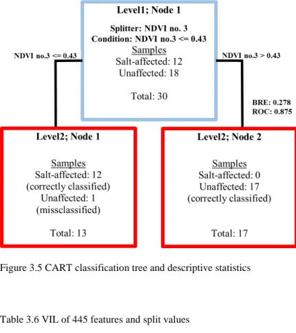
Table 3.6 VIL of 445 features and split values ... 51
Table 4.1 Salinity tolerances of dominant crops in the Vaalharts and Breede River irrigation schemes. Threshold A is the maximum root zone salinity at which 100% yield occurs. Slope B is the reduction in relative yield per increase in soil salinity. ... 60
Table 4.2 SPOT-5 bands and spatial resolution ... 61
Table 4.3 Histex algorithms as implemented by the PCI software ... 65
Table 4.4 Indirect indicator feature sets considered ... 66
Table 4.5 Regression models and algorithms ... 67
Table 4.6 Supervised classifiers considered and their implementations ... 68
Table 4.7 Six most important variables in Vaalharts according to CART and RF respectively ... 72
Table 4.8 Six most important variables in Breede River according to CART and RF respectively ... 72
Table 4.9 Summary of average and individual classifiers for Vaalharts ... 73
Table 4.10 Summary of average and individual classifiers for Breede River ... 74
Table 5.1 SPOT-5 scenes acquired for the study areas ... 84
Table 5.2 Vaalharts irrigation scheme error matrix ... 91
Table 5.3 Loskop irrigation scheme error matrix ... 91
Table 5.4 Makhatini irrigation scheme error matrix ... 91
Table 5.5 Tugela irrigation scheme error matrix ... 91
Table 5.6 Olifants River irrigation scheme error matrix ... 92
Table 5.7 Breede River irrigation scheme error matrix ... 92
Table 5.8 Sondags River irrigation scheme error matrix ... 92
Table 5.9 Pondrift irrigation scheme error matrix ... 92
Table 5.10 Douglas irrigation scheme error matrix ... 92
FIGURES
Figure 1.1 Induced secondary salinization in irrigated areas ... 3 Figure 1.2 Examples of a) white efflorescent salt crust and b) surface ponding (waterlogging) in
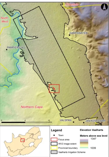
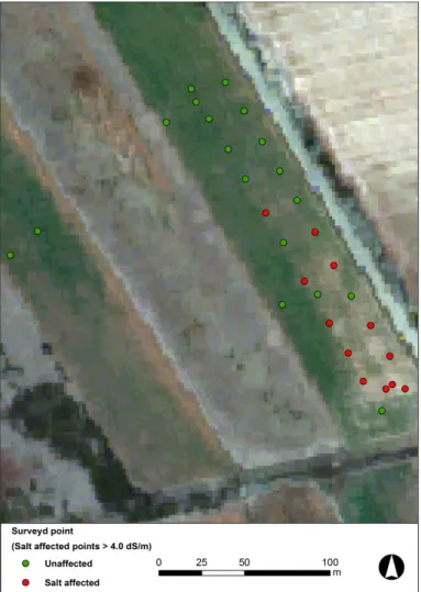
the Vaalharts irrigation scheme. ... 5 Figure 1.3 Research design and thesis structure ... 13 Figure 2.1 Electromagnetic spectrum and its relation to passive and active remote sensors. ... 15 Figure 2.2 Instantaneous field of view of a satellite sensor capturing data at nadir and of-nadir . 17 Figure 2.3 Spectral reflectance of healthy vegetation ... 29 Figure 3.1 Study site location within the Vaalharts irrigation scheme ... 38 Figure 3.2 Surveyed points of the grid-based sampling approach. The adjacent field consists
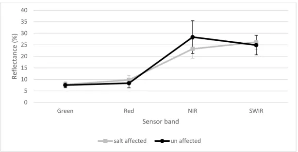
similarly of lucerne and orthic Kimberly soil ... 41 Figure 3.3 Spectral profile of salt-affected and unaffected vegetation. The series represents the
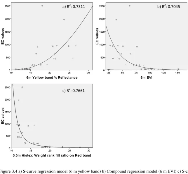
mean response of the surveyed points where 4.0 dS/m separates salt-affected vegetation from unaffected vegetation (error bars represent one standard deviation) ... 48 Figure 3.4 a) S-curve regression model (6 m yellow band) b) Compound regression model (6 m
EVI) c) S-curve regression model (0.5 m B12) ... 50 Figure 3.5 CART classification tree and descriptive statistics ... 51 Figure 4.1 Study area map ... 59 Figure 4.2 Spectral profiles of salt-affected (n = 19; EC >4.0 dS/m) and unaffected (n = 50; EC <
4.0 dS/m) vegetation as extracted from the SPOT-5 image of Vaalharts with error bars indicating one standard deviation ... 70 Figure 4.3 Spectral profiles of salt-affected (n = 23; EC > 4.0 dS/m ) and unaffected (n = 25; EC
< 4.0 dS/m) vegetation as extracted from the SPOT-5 image of the Breede River with error bars indicating one standard deviation ... 71 Figure 4.4 DT classification results (a and c) using Feature Set G in two detail areas within the
Vaalharts irrigation scheme. On the right true colour images of the same areas are provided for comparison purposes (b and d). ... 75 Figure 4.5 SVM classification result using Feature Set D in two detail areas within the Breede
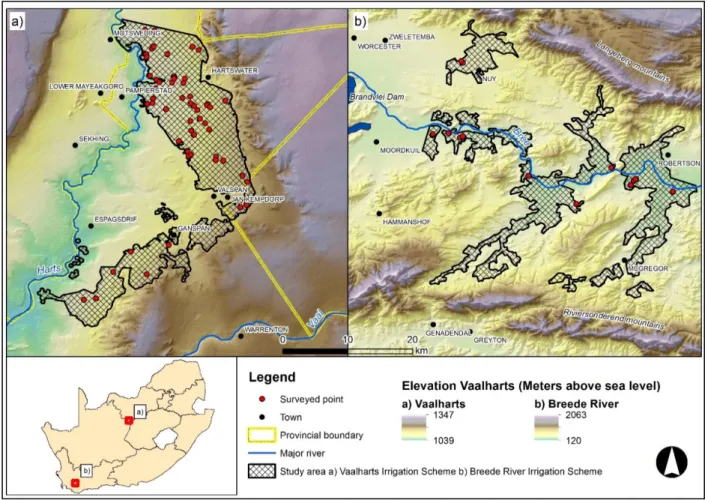
River irrigation scheme (a and c). On the right true colour image combination (b and d) ... 77 Figure 5.1 Geographical distribution of the nine irrigation schemes across South Africa, with
elevation data as backdrop ... 83 Figure 5.2 Hierarchical WFAD segmentation process ... 87
Figure 5.3 Mean difference threshold process. a) Parent level segmentation with mean NDVI value b) Child level segmentation with individual NDVI values c) Identified
anomalies with MeaD equation when a threshold of -0.07 is applied. ... 88 Figure 5.4 Indication of the extent of anomaly delineation for four areas, with a and b
representing examples of good delineations and c and d highlighting some
ACRONYMS AND ABBREVIATIONS
ANOVA Analysis of variance
ARC ASTER
Agricultural Research Council
Advance space-borne thermal emission and reflection radiometer
AUC Area under the curve
AVIRIS BR
Airborne visible infrared imaging spectrometer Brightness ratio
BRE Best relative error
CART Classification and regression tree
CASI CBERS
Compact airborne spectrographic imager China-Brazil earth resources satellite
COSRI Combined spectral response index
DEM Digital elevation model
DN Digital numbers
DT Decision tree
EC Electroconductivity
EM Electromagnetic
ETM Enhanced thematic mapper
EVI FAO
Enhanced vegetation index
Food and Agriculture Organization
FCC False colour composite
GCP Ground control points
GEOBIA Geographical object-based image analysis
GIS Geographical information system
GLCM Grey level co-occurrence matrix
GLDV Grey level difference vector
GPS Global positioning system
GVMI General vegetation moisture index
IHS Intensity, hue, and saturation
IRS Indian remote sensing
IFOV Instantaneous field of view
KC Kappa coefficient
KZN LiDAR
KwaZulu-Natal
Light detection and ranging
LISS Linear imaging self-scanning system
LMM Local mean matching
LMVM Local mean and variance matching
LO Longitude of origin
LSU MeaD
Linear spectral unmixing Mean difference
MinD Minimum distance
ML Maximum likelihood
MODIS MRS
Moderate resolution imaging spectroradiometer Multi-resolution segmentation
NDVI Normalized difference vegetation index
NIR Near-infrared
NN Nearest neighbour
OA Overall accuracy
OBIA Object-based image analysis
OI Optical imagery
PA Producer’s accuracy
PCA Principal component analysis
PLS Partial least squares
PRI RADAR
Physiological reflectance index Radio detection and ranging
RF Random forests
RGB Red, green, blue
RSA Republic of South Africa
ROC Receiver operating characteristics
RVI Ratio vegetation index
SAM Spectral angle mapper
SANSA South African National Space Agency
SAVI Soil-adjusted vegetation index
SEBAL Surface balance algorithm for land
SFF Spectral feature fitting
SMA Spectral mixture analysis
SMR Stepwise multiple regression
SPOT Satellite pour l’observation de la terre
SVM Support vector machine
SWIR Shortwave infrared
SWSI TIR
Salinity and water stress indices Thermal infrared
TM Thematic mapper
US User’s accuracy
USDA United States Department of Agriculture
VHR Very high resolution
VIL Variable importance list
VIs Vegetation indices
VIS Visible spectrum
WFAD Within-field anomaly detection
WI Water index
WRC Water Research Commission
CHAPTER 1:
INTRODUCTION
Soil salinity, for the purpose of this study, is defined as the accumulation of soluble salts in the topsoil. Salinity can be classified as primary (i.e. when soil salinity occurs naturally), or secondary (when induced by human interference). Secondary salinity mainly occurs due to a lack of proper planning or maintenance of irrigation infrastructures and is a major concern, especially in irrigated areas. Extreme salt accumulation leads to the death of vegetation and consequently to a reduction in crop yield and general degradation of fertile soil (Ghassemi, Jakeman & Nix 1995). Previous estimates of global salinity effects indicate that around 77 million hectare of the earth’s surface is affected by secondary salinity and that more than half of this area is made up of irrigated soil (Metternicht & Zinck 2003). The negative economic impact of salt-affected soils on the agricultural sectors’ production capacity is immense, with the added pressure of maintaining sustainable food production in a world with a growing population. With quality crop and soil management, good irrigation and drainage systems design and political and social support, irrigation can be a thriving, sustainable practice (Hillel & Vlek 2005; Van Rensburg et al. 2012). Quality management practice includes tracking and identifying salinity changes to anticipate further degradation and to undertake suitable reclamation and rehabilitation practices (Metternicht & Zinck 2003).
1.1 SOIL SALINITY
The term salinity is used to describe both the processes and impacts of salt on soil and water, while also being a measure of the amount of salt in soil or water (Hillel 2000; McGhie & Ryan 2005). The electrolytic mineral solutes most commonly associated with salinity are the cations Na+, K+, Ca2+ and Mg2+ and the anions Cl-, SO42-, NO, HCO and CO32- (Hillel 2000). The
sources and processes of salt accumulation are vast and dynamic. Soil salinity can occur naturally (primary) or as a result of human interference (secondary) (Ghassemi, Jakeman & Nix 1995). Salts occur naturally in soils formed in arid regions simply because they have not been leached by rain (Hillel 2000). However, the salt content in such soils depends greatly on the nature of the soil. The salt content for sandy soils is generally lower than that of soils with a high content of clay minerals (Ghassemi, Jakeman & Nix 1995). Brackish groundwater can also infuse salts into top soil, typically where the subsoil contained accumulated salts from previous geologic eras. Rising water tables can transport these salts from the subsoil to the crop root zone. Rainwater is also considered a natural cause and can indirectly contribute to soil salinity, especially near industrialized regions where rainwater mixes with emitted gasses, or near coastal regions where sea spray can mix with rainwater.
The more insidious form of soil salinity occurs when previously productive soils are subjected to salinity due to human interference. This secondary salinity is mainly due to the extra water provided by human activities, such as irrigation and land clearing (Ghassemi, Jakeman & Nix 1995).
Some of the processes that give rise to human-induced salinity include:
When water containing mineral salts is used for irrigation, the salts are transported to the crop root zone. Through the processes of transpiration and evaporation, the water is returned to the atmosphere and the salts are left behind in the soil. Highly arid regions require more irrigation and have less rainfall to leach out the accumulated salts (Hillel 2000; Umali 1993).
Irrigation in poorly drained areas leads to increased water infiltration and the rising of the natural water table (Ghassemi, Jakeman & Nix 1995). This effect is exacerbated by the over-application of irrigation water, which especially happens when water is priced below its true economic value (Umali 1993). Similar to the natural process, the rising water table (artificial rise) leads to the transportation of salts to the crop root zone.
Irrigation systems often have an intricate canal system for the transportation of irrigation water. The canals are mostly unlined and have a high seepage rate. The infiltrating water accumulates and over time can raise the water table to within a few metres of the land surface (Ghassemi, Jakeman & Nix 1995).
A change in the hydrological balance that occurs when land is cleared for farming and pastoral activities can be another major cause of rising water tables. When land is cleared, the deep-rooted natural vegetation is removed, leading to less evapotranspiration. Consequently, more water infiltrates the soil, supplementing the natural water table (Ghassemi, Jakeman & Nix 1995).
An overview of secondary salinity, specifically in irrigated areas, is shown in Figure 1.1. Umali (1993) ascribes most of the human-induced salinity to poor water-use efficiency on farms owing to a lack of awareness; poor engineering and maintenance on the canal systems (leading to increased seepage); insufficient or non-existing artificial drainage infrastructure; and poor design and maintenance of artificial drainage infrastructure. In irrigation schemes, most salt accumulation occurs as a result of the secondary process.
Source: Abbas et al. (2013)
Figure 1.1 Induced secondary salinization in irrigated areas
1.1.1 Waterlogging
Waterlogging, a process very closely related to soil salinity (Figure 1.1), is the saturation of the soil as a result of the water table being located at or near the surface (Barrett-Lennard 2003; McDonagh & Bunning 2009). The secondary salinity processes that lead to a rising water table similarly contributes to the occurrence of waterlogging. Waterlogging can also be caused by high sodicity levels in soils, which limit the infiltration of surface water as a result of compaction and crusting (Ghassemi, Jakeman & Nix 1995; Qureshi & Barrett-Lennard 1998). Soil sodicity occurs when clay particles in the soil becomes dominantly charged with sodium (Na) ions, rather than calcium (Ca) ions (Hillel 2000; Qureshi & Barrett-Lennard 1998).
1.1.2 Effects and indicators of soil salinity and waterlogging
Halophytic plants are adapted to grow in saline conditions (Hillel 2000; Qureshi & Barrett-Lennard 1998). Some of these plants only occur in saline conditions and can therefore be used to identify areas affected by salt accumulation. These salinity indicator plants, however, vary between different regions (McGhie & Ryan 2005). Glycophytes, plants that are not adapted to survive in saline conditions, show indications of physiological stress in the presence of salinity. Most crop plants are glycophytic (Hillel 2000).
If the accumulation of salts in the root zone is higher than the plant’s tolerance level, the plant will have a reduced ability to take up water. The plant then goes into an “osmotic adjustment”
Seepage from supply system
Irrigation with varying degree of salt concentrations Salts build up in the
soil profile
Leaching requirements
Extra water is applied
Water logging appears and leaching ceases Capillary rise takes place
Salt-affected soils Crop growth is restricted Damage of soil structure Ionic unbalance Ionic
process, using additional metabolic energy (i.e. from photosynthesis) in an attempt to take up more water (Hillel 2000). This inevitably leads to the dehydration and wilting of plant leaves and stems, known as the osmotic effect (McGhie & Ryan 2005).
When a plant absorbs water and nutrients during transpiration, small amounts of salt will accompany the water. In persistent saline conditions, over time, these salts will accumulate and may have a toxic effect on the plant. Some of the ions related to salinity that cause the toxic effect are an abundance of chloride (Cl-) and sodium (Na+) (Hillel 2000). The toxicity can lead to internal structural damage and more commonly leads to leaf injury symptoms (leaf tips of plants turn yellow) (Hillel 2000; McGhie & Ryan 2005).
In the case of waterlogging, there is an oxygen deficiency in the soil due to the low solubility and diffusivity of oxygen in the water, which causes a state of hypoxia (Armstrong et al. 1991; Barrett-Lennard 2003). Since plant roots require oxygen for optimal production, the lack thereof results in a rapid decrease of growth, the loss of its ability to screen out salts at the root zone and the loss of its ability to absorb organic nutrients. Physiological indicators include discolouring of vegetation, defoliation, wilting and plant death (Barrett-Lennard 2003; McGhie & Ryan 2005; Qureshi & Barrett-Lennard 1998). McGhie & Ryan (2005) observed that waterlogging symptoms are very similar to those caused by an excess of salt.
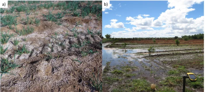
It should be clear from the above discussion that physiological vegetation stress is a potential indicator of salinity and waterlogging. There are also other, more direct, indicators of salinity and waterlogging. For instance, a white efflorescent salt crust on the soil surface is a direct sign of salt accumulation (McGhie & Ryan 2005). These efflorescent salt crusts form when saline water evaporates and salts crystalize on soil grains (Goodall, North & Glennie 2000). This results in a powdery or puffy texture that has a high reflectance (i.e. appear bright) (Metternicht & Zinck 2003) (Figure 1.2a). Other surface features of salinity include: black staining when iron in the soil reacts with sulphate salts (SO42-), bare patches without salt encrustations and soil
erosion due to the loss of protective vegetation cover. Waterlogging is directly detectable on the surface in the visible saturation of the topsoil and surface ponding (Figure 1.2b) (Dwivedi, Sreenivas & Ramana 1999). When the water of a surface pond evaporates, salt encrustation also tends to form.
1.1.3 Salinity impacts
In an advanced stage, the cumulative effects of soil salinity and waterlogging on its surroundings can lead to adverse agricultural and environmental impacts. If salinity reaches high levels, it kills off all vegetation, resulting in reduced crop yield and quality, and renders the once fertile soil barren, stripped of any biodiversity (Ghassemi, Jakeman & Nix 1995). Salinity is not as dramatic or damaging as earthquakes or landslides, yet it is still one of the most severe environmental factors impairing the production of agricultural crops (Ghassemi, Jakeman & Nix 1995; Metternicht & Zinck 2003; Pitman & Läuchli 2002; Umali 1993; Zinck 2000).
Estimations of the extent of salt-affected areas vary greatly. Metternicht & Zinck (2003) estimated that primary salinity covers a total of 1 billion hectares of the earth surface – about 7% of the earth’s continental extent Secondary salinity accounts for an additional 77 million hectares, with 58% occurring in irrigated areas. According to Hillel (2000), irrigated cropland makes up 17% of cropland globally, while contributing 30% of the total agricultural production – highlighting the importance of irrigation and the impact that secondary salinity can have on food security. Ghassemi, Jakeman & Nix (1995) estimate that 20% of these irrigated croplands are salt-affected. Globally, the economic impact of the loss in production capacity due to salinity is estimated at $US 11.4 billion and $US 1.2 billion per year in irrigated and dryland areas respectively (Ghassemi, Jakeman & Nix 1995). A more recent global estimate is urgently needed, especially given that dryland crops are increasingly being converted to irrigated agriculture to increase agricultural production, which could lead to a dramatic increase in induced soil salinity (Metternicht & Zinck 2003). Other problems linked to soil salinity includes
Figure 1.2 Examples of a) white efflorescent salt crust and b) surface ponding (waterlogging) in the Vaalharts irrigation scheme.
losses in property values, eutrophication of rivers, damage to infrastructure, increased soil erosion and engineering difficulties (Metternicht & Zinck 2003).
1.1.4 South African situation
In South Africa, the total area under irrigation is estimated at 1.3 million ha. Irrigation is critical for food security, specifically given that large parts of the country receives insufficient rainfall for dryland crop production (Backeberg 2003; Backeberg et al. 1996). In the comprehensive literature review by Ghassemi, Jakeman & Nix (1995), it is estimated that up to 9% of South African irrigated lands are susceptible to salt accumulation. Backeberg et al. (1996) reported that between 1% and 12% of the South African irrigation schemes suffer from severe waterlogging and salt accumulation, while between 5% and 20% are moderately affected. This percentage is much lower compared to other regions such as Argentina (34%), Egypt (33%), Iran (30%), Pakistan (26%) and USA (23%) (Ghassemi, Jakeman & Nix 1995). This favourable status is attributed to careful selection of irrigated areas, good drainage and the smaller sized irrigated areas in South Africa. Although the extent of salt-affected areas in South African irrigation schemes is less severe, Ghassemi, Jakeman & Nix (1995) warns that the salinization of reservoirs used for water supply can have a direct effect on salt accumulation in irrigation schemes. Also, there is no active programme in place to monitor the extent and changes in salt-affected and waterlogged areas (De Villiers et al. 2003). Such complacency can potentially lead to conditions that may cumulatively cause rapid salt accumulation and loss of scarce productive land.
1.1.5 Importance of irrigated agriculture
Irrigation is necessary for the sustainable maintenance of food production in South Africa. For example, the fruit and wine industries of the Western Cape are entirely dependent on irrigation, while cropping in the Eastern and Northern Cape also rely heavily on irrigation (Van Rensburg et al. 2011). The posing threat of salinity in irrigation schemes is real, but manageable. Letey (1994), Rhoades (1997) and Van Schilfgaarde (1990) as cited in Van Rensburg et al. (2012) are all in agreement that sustainable irrigation is possible with well-designed irrigation and drainage systems, good crop and soil management practices and support from political and social structures. These factors can, according to Hillel & Vlek (2005), help to strengthen irrigated agriculture and increase food production.
Pressure on agricultural land increases with an increase in population (currently at 1.6% per annum). Irrigation schemes account for almost 30% of the total crop production (De Villiers et al. 2003). Saline soils pose a threat to sustainable agriculture and can significantly reduce crop
yields – particularly in irrigation schemes. There is consequently a need for a systematic management of salt accumulation to mitigate further losses of fertile agricultural land. Salt accumulation management practice require monitoring to anticipate degradation and to make informed decisions about reclamation and rehabilitation (Metternicht & Zinck 2003). Monitoring includes identifying locations of salt accumulation and tracking its temporal and spatial dynamics.
1.1.6 Salt accumulation monitoring
An area’s salinity status is usually determined by carrying out field surveys and performing laboratory analyses of collected soil samples. There are a number of ways to measure the salt content in soils. The saturated paste technique is widely used for measuring the salt content in a soil sample, and has shown sufficient accuracy. The process involves extracting the salt concertation of a soil sample with the use of water to ultimately determine its electroconductivity (EC). Electroconductivity is defined as the degree to which water conducts electricity, which is proportional to the amount of salts in the solution (Hanson, Grattan & Fulton 2006). The measured EC value is widely used as an indicator of soil salinity. In South Africa, soil samples with EC values of 4.0 dS/m (deci-siemens per metre) or higher are regarded as being salt-affected, while all samples with EC values below 4.0 dS/m are regarded as being unaffected (Bresler, McNeal & Carter 1982; Richards 1954; SASA 2007).
Conventional methods for monitoring salt accumulation are laborious and costly and not viable when frequent monitoring is required over extensive (e.g. national) areas. A cost-effective solution for monitoring salt accumulation over large areas is consequently needed.
1.1.7 Earth observation for monitoring soil salinity
Earth observation by remote sensing can capture data on both a temporal and spatial scale and has the potential for identifying salt-affected areas. If successfully applied, remote sensing can serve as a monitoring solution that would not be as costly and labour intensive as regular field surveys and laboratory analyses.
Various techniques and applications of remote sensing for the identification of salt-affected areas have been published. Salt accumulation can be detected either directly or indirectly using remotely sensed images (Bastiaanssen 1998; Mougenot, Pouget & Epema 1993). The direct detection of the accumulation of salts involves identifying salt encrustations on the bare ground, while the indirect method focuses mainly on vegetation responses to salt accumulation.
Several authors have successfully applied the direct approach for identifying salt accumulation (Abood, Maclean & Falkowski 2011; Dwivedi & Sreenivas 1998; Elnaggar & Noller 2010; Iqbal 2011; Khan et al. 2005; Metternicht & Zinck 2003; Rao et al. 1995; Setia et al. 2013; Sidike, Zhao & Wen 2014). Most of these studies reported that salt crusts generally have high reflectance in the visible and near to mid-infrared regions of the electromagnetic spectrum, depending on the chemical composition of the salts (Metternicht & Zinck 2009). Specific spectral ranges for direct salinity detection (identified by laboratory analyses) are in the visible region (550-770 nm), near-infrared region (900-1030 nm, 1270-1520 nm) and middle infrared region (1940-2150 nm, 2150-2310 nm, 2330-2400 nm) (Csillag, Pasztor & Biehl 1993). Metternicht & Zinck (2009) observed that applying laboratory techniques to optical remote sensing data to detect salt accumulation is complicated by the variations in reflectance that cannot be attributed to a single soil property and salt type. Spectral variation in salt crusts can be attributed to the difference in the quantity of salts, the mineralogy of the salts (e.g. carbonates, sulphates or chlorides), soil moisture, colour of the salt crust (white to dark) and surface roughness of the salt crust (smooth to rough), which all vary among chemical structures. The direct approach also fails to take into account salt accumulation that occurs in the sub-surface, since it is limited to monitoring surface conditions.
The indirect approach, which focuses mainly on vegetation monitoring, has also been successfully applied to remotely identify salt-affected areas. One approach is to identify halophytic vegetation types that commonly occur in salt-affected areas (Dehaan & Taylor 2002; Dehaan & Taylor 2003; Dutkiewicz, Lewis & Ostendorf 2009a; García Rodríguez, Pérez González & Guerra Zaballos 2007). However, this method is less suitable for application in irrigated areas where natural vegetation is removed during field preparations. A more common approach in irrigated areas is to monitor vegetation (crop) vigour. For this purpose, vegetation indices (VIs) are primarily used to distinguish between healthy vegetation and stressed vegetation. Two of the most used VIs are the NDVI (Abbas et al. 2013; Aldakheel 2011; Bouaziz, Matschullat & Gloaguen 2011; Elnaggar & Noller 2010; Hamzeh et al. 2012a; Platonov, Noble & Kuziev 2013; Sidike, Zhao & Wen 2014; Zhang et al. 2011) and the SAVI (Abood, Maclean & Falkowski 2011; Allbed, Kumar & Aldakheel 2014; Bouaziz, Matschullat & Gloaguen 2011; Elnaggar & Noller 2010; Hamzeh et al. 2012b; Koshal 2010; Zhang et al. 2011). However, using vegetation response for identifying salinity conditions should be used with caution because many factors besides soil salinity (e.g. farming practices) can contribute to loss of vegetation vigour (Metternicht & Zinck 2009). Different crops in different growing phases
also have different tolerances to soil salinity, which further complicates the implementation of the indirect approach.
1.2 PROBLEM FORMULATION
Conventional methods of monitoring the accumulation of salts include soil surveys and laboratory analyses. These methods are not practical for systematic monitoring over large areas. Earth observation has been shown to be effective for monitoring salt-affected areas by detecting vegetation stress caused by exposure to high levels of salts in the soil. Previous applications of the indirect approach have been carried out successfully in areas where soil salinity occurs at a grand scale (i.e. high levels of salinity and large affected areas). As a result, the satellite imagery most commonly employed for detecting soil salinity has low to medium spatial resolution. Examples include 30 m Landsat (Abdelfattah, Shahid & Othman 2009; Aldakheel 2011; Dehni & Lounis 2012; Gao & Liu 2008; Mohamed, Morgun & Goma Bothina 2011); 23 m IRS (Abbas et al. 2013; Dwivedi et al. 2001; Dwivedi & Sreenivas 1998; Eldiery, Garcia & Reich 2005; Khan et al. 2001; Koshal 2010) and 250 m MODIS (Lobell et al. 2010). Given the relatively small field sizes (e.g. 2 ha) in South African irrigation schemes and the narrowness of affected areas (generally only a few metres in width) (Nell et al. 2015), medium to low resolution imagery will be of little value for monitoring salt accumulation in South African irrigation schemes.
The increasing availability of high resolution satellite imagery enables the assessment of the extent to which remote sensing can detect saline soils beyond the medium and low resolution image domains. Very high resolution (VHR) satellite imagery consequently provides a greater amount of spatial information, which enables the use of sophisticated data mining and image analysis techniques. Finding the optimal combination of high resolution imagery and image analysis techniques for indirectly identifying salt accumulation in South African irrigation schemes would greatly benefit a systematic salinity monitoring approach. A literature review of published remote sensing and salt accumulation research revealed that no research has yet been done on the use of VHR imagery for indirectly identifying small patches of affected areas (such as those occurring in South Africa) in irrigation schemes. Early detection of affected areas (i.e. while they are still small) will facilitate the implementation of mitigating measures and may prevent losses of fertile agricultural land.
From a research perspective, very little is known about the optimal combinations of VHR spectral bands for detecting salt-affected areas. It is also not clear which image analysis
techniques are best for indirectly identifying salt accumulation. The following research questions were consequently set:
1. What spatial and spectral resolutions would be suitable for the indirect detection of salt-affected areas in a typical South African irrigation scheme?
2. Would the identified spatial and spectral resolutions be viable and robust for implementation over large areas?
3. To what extent would the dynamic nature of crops and their varying salinity tolerance influence the indirect monitoring of salt accumulation?
4. What observation scale (field level or scheme level) would be the most efficient for indirectly detecting salt accumulation over large areas?
5. Which image transformations and classification techniques are most robust (transferable) for indirectly identifying salt accumulation across multiple irrigation schemes?
1.3 RESEARCH AIM AND OBJECTIVES
The primary aim of this research is to implement and assess indirect earth observation approaches for detecting salt accumulation in soils, with a particular focus on irrigation schemes. The secondary aim is to develop and evaluate an earth observation methodology in the context of finding operational solutions for monitoring salt accumulation in South African irrigation schemes.
To achieve the research aim, the objectives are to:
1. review the literature on detecting salt accumulation using earth observation;
2. collect and prepare in situ reference data and acquire suitable remotely sensed imagery; 3. assess the value of high (spectral and spatial) image resolution for indirectly identifying
salt accumulation in a single cultivated field;
4. identify the image features and classification techniques most successful in discriminating between salt-affected and unaffected areas at irrigation scheme level; 5. develop and demonstrate a semi-automated, transferable earth observation methodology
for monitoring salt accumulation in South African irrigation schemes; and
6. critically evaluate the developed methodology in the context of finding operational solutions for monitoring salt-affected areas in South African irrigation schemes.
1.4 RESEARCH METHODOLOGY AND THESIS STRUCTURE
The research approach was deductive and experimental in nature. The quantitative analyses included statistical techniques (regression analysis), machine learning (decision trees, k-nearest neighbour, random forest, and support vector machines) and expert systems (rule-based classification models). Two experiments were carried out using empirical datasets obtained from in situ field surveys and remotely sensed imagery.
The first experiment focused on a single field analysis and aimed to contribute towards research questions one, two, four and five. The main aim of the experiment was to determine the optimal spatial and spectral resolutions required for identifying salt accumulation in a typical irrigated field. The experiment used empirically measured in situ EC data and WoldView-2 (WV2) imagery. The data was quantitatively analysed using regression modelling and a decision tree algorithm.
The second experiment was carried out at irrigation scheme level and aimed to contribute towards research questions three, four and five. Two irrigation schemes were selected for examining the influence of variations in crop type and salt tolerance on detecting affected areas. This experiment also aimed to identify specific image transformation or classification techniques that are consistently effective at monitoring soil salinity at irrigation scheme level. Empirically measured in situ EC data and SPOT-5 satellite imagery were used as main data sources. The data was quantitatively analysed using regression modelling, decision tree analysis and image classification techniques. The findings of the two experiments were applied in an inductive spatial modelling approach in order to develop a robust (i.e. transferable) salinity monitoring technique.
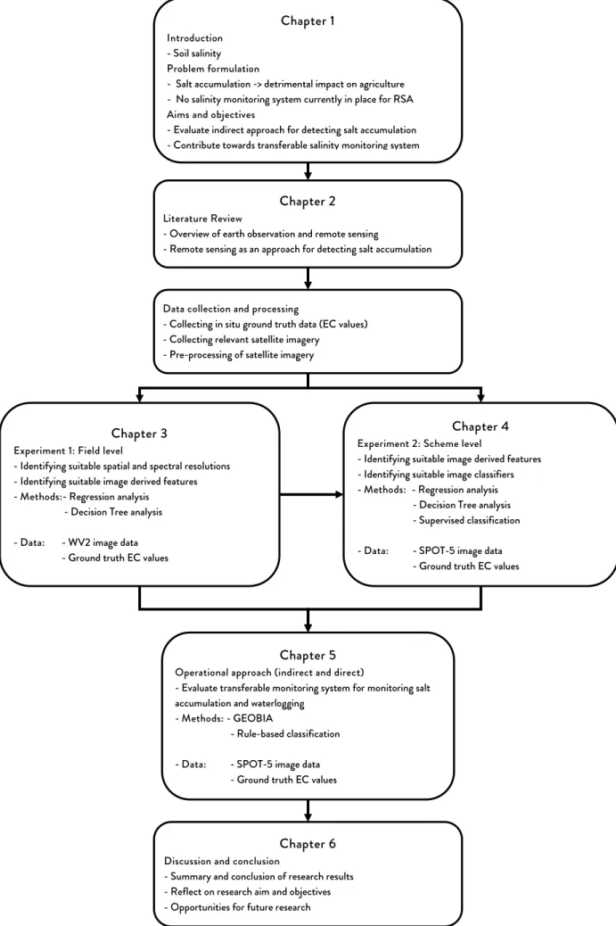
Figure 1.3 outlines the research design and illustrates how it relates to the thesis structure. The real world problem and research questions, together with the research aims and objectives, were outlined in this chapter. Chapter 2 provides an overview of earth observation and remote sensing, followed by a review of how remote sensing techniques have been used to detect salt accumulation.
Chapters 3 and 4 present the two experiments that evaluated the indirect earth observation approach’s capability to detect salt accumulation at a field and a scheme level respectively. Chapter 5 builds on the knowledge gained from the two experiments, and proposes a robust and transferable monitoring technique. Chapters 3 and 4 are structured as independent research articles and consequently include theoretical discussions as well as overviews of the study areas,
datasets and quantitative methods used. Repetition of certain concepts and methods was consequently unavoidable.
Chapter 6 provides a summary and a critical evaluation of the research. It reflects on the research questions, aims and objectives, and discusses the key findings in the context of establishing an operational solution for monitoring salt accumulation in irrigated areas. Recommendations for further research are also made.
The next chapter provides a brief overview on the concepts of earth observation and remote sensing. Applications of remote sensing for detecting salt accumulation, identified in published literature, are then discussed.
Figure 1.3 Research design and thesis structure
Chapter 1
Introduction - Soil salinity Problem formulation
- Salt accumulation -> detrimental impact on agriculture - No salinity monitoring system currently in place for RSA Aims and objectives
- Evaluate indirect approach for detecting salt accumulation - Contribute towards transferable salinity monitoring system
Chapter 2
Literature Review
- Overview of earth observation and remote sensing
- Remote sensing as an approach for detecting salt accumulation
Data collection and processing
- Collecting in situ ground truth data (EC values) - Collecting relevant satellite imagery
- Pre-processing of satellite imagery
Chapter 3
Experiment 1: Field level
- Identifying suitable spatial and spectral resolutions - Identifying suitable image derived features - Methods:- Regression analysis
- Decision Tree analysis - Data: - WV2 image data
- Ground truth EC values
Chapter 4
Experiment 2: Scheme level
- Identifying suitable image derived features - Identifying suitable image classifiers - Methods: - Regression analysis
- Decision Tree analysis - Supervised classification - Data: - SPOT-5 image data
- Ground truth EC values
Chapter 5
Operational approach (indirect and direct)
- Evaluate transferable monitoring system for monitoring salt accumulation and waterlogging
- Methods: - GEOBIA
- Rule-based classification - Data: - SPOT-5 image data
- Ground truth EC values
Chapter 6
Discussion and conclusion
- Summary and conclusion of research results - Reflect on research aim and objectives - Opportunities for future research
CHAPTER 2:
EARTH OBSERVATION FOR SALINITY DETECTION
An understanding of salinity, its causes, effects and dynamic processes, together with remote sensing and its capabilities, was vital for achieving the aims and objectives of this study. The first section of this chapter consequently summarizes relevant earth observation concepts, while the rest of the chapter is dedicated to a review of remote sensing applications for detecting soil salinity.
2.1 EARTH OBSERVATION
Earth observation is a wide-ranging term used to describe remote sensing and geographical information systems (GIS) technologies and applications. Remote sensing is widely defined as attaining and recording information about a specific object without being in direct contact with it (Campbell 2007; Fischer, Hemphill & Kover 1976; Gibson 2000). For this study, it is more specifically defined as acquiring information about the earth’s surface with satellite sensors by recording electromagnetic radiation through one or more regions of the electromagnetic spectrum reflected from the earth’s surface (Campbell 2007). A GIS refers to a computerized system for capturing, storing, querying, analysing and displaying geospatial data (Chang 2010).
2.1.1 Electromagnetic spectrum
Electromagnetic (EM) energy, most commonly experienced as visible light, consists of two oscillating components, namely electric and magnetic fields (Tempfli et al. 2009). Electromagnetic energy is measured by its wavelength or frequency unit (Figure 2.1). This energy is generated by all matter with an absolute temperature above zero (Tempfli et al. 2009). The sun, however, is the prime source of this energy and produces a full spectrum of electromagnetic radiation, known as the electromagnetic spectrum. Of this full range, the visible spectrum only encompasses one ten-thousandth of one percentage of the total range (Gibson 2000). As the electromagnetic energy passes through the atmosphere to interact with objects on the earth’s surface, its behaviour changes. The levels of reflection and absorption of each object on the earth’s surface vary and each object uniquely interacts with the EM energy. By recording the changes in how surface objects behave under different EM energy spectra, scientists can attain knowledge of the different characteristics of objects (e.g. vegetation cover, water bodies, soils or urban structures) by using remotely sensed data (Campbell 2007). The most relevant regions of the electromagnetic spectrum for remote sensing applications are described by Chuvieco & Huete (2010) as the visible (VIS), near-infrared (NIR), shortwave infrared (SWIR) and thermal infrared (TIR) regions.
The VIS, with wavelengths ranging from 0.4 to 0.7 micrometres (μm), is named after the energy that human eyes are capable of sensing. It includes the blue, green and red areas of the spectrum (Figure 2.1). This part of the spectrum is also used to visualize the EM energy humans cannot directly see.
The NIR includes wavelengths of 0.7 to 1.2 μm, is invisible to humans and is well-known for its ability to record green vegetation. Healthy vegetation has a high reflectance in this region and reflectance decreases with increased plant stress (Tempfli et al. 2009).
The SWIR is delimited by 1.2 and 3 μm wavelengths and is known for its vegetation and soil moisture identification.
With wavelengths longer than the 3 μm, the TIR is associated with emissive electromagnetic radiation from the earth’s surface. The earth’s surface has a peak wavelength of 10 μm (Tempfli et al. 2009).
The shortest microwave wavelengths have properties similar to the thermal region and the longest wavelengths merge into radio wavelengths used for commercial broadcasts (Campbell 2007). The microwave wavelengths are commonly known for its capability to penetrate cloud cover.
Source: SEOS (2016) Figure 2.1 Electromagnetic spectrum and its relation to passive and active remote sensors.
2.1.2 Active (microwave) vs passive (optical) sensors
Remote sensors, the physical devices that detect EM energy, can be grouped into two main types, namely passive and active remote sensors. A passive remote sensor measures solar energy reflected from or radiation emitted by the earth’s surface. To detect solar energy reflected from the earth’s surface, instruments (known as optical sensors) must be capable of recording in the visible and preferably also in near-infrared spectrum. Some of the key variables in the process of capturing data with these sensors are atmospheric clarity, spectral properties of objects, angle and intensity of the sun, and choices of films and filters (Campbell 2007). To detect radiance emitted from the earth’s surface, instruments (known as thermal sensors) must be capable of recording in the thermal infrared region. These sensors are also considered passive because they do not create electromagnetic energy themselves, but only record what is reflected or emitted from the earth.
An active remote sensor emits its own EM energy and then detects the energy returned from the target object or surface (Tempfli et al. 2009). Active remote sensors are independent of solar and terrestrial radiation and can thus operate during day or night. These sensors are represented by the NIR region, in the form of light detection and ranging (LiDAR) instruments, and the microwave region, in the form of radio detection and ranging (RADAR) instruments. The latter has wavelengths long enough to penetrate could cover.
2.1.3 Characteristics of optical imagery
Satellite sensors capture the reflected or emitted electromagnetic energy and convert it into a grid array of cells (pixels). Each pixel contains a raw digital number (DN), representing the amount of reflectance/emittance of a specific region in the electromagnetic spectrum (VIS, NIR or SWIR). This specific region is commonly known as a sensor band. The collective array of pixels forms a raster image, used for analysis. Each raster image is uniquely defined by certain characteristics relative to its satellite system, which ultimately determines its value for specific remote sensing problems. These characteristics are spatial, spectral, temporal and radiometric resolution.
Spatial resolution refers to the detail visible in an image, e.g. what is the smallest object detectable on the ground surface. For satellites, it is primarily determined by its instantaneous field of view (IFOV) (Figure 2.2) and measured by metres on the ground (Chuvieco & Huete 2010; Gibson 2000). The spatial resolution of satellite images can range from a few centimetres to kilometres, depending on the satellite system.
Spectral resolution determines how many sensor bands are provided. A larger spectral resolution means a greater coverage of the electromagnetic spectrum, which enables a better recording of surface objects’ spectral characteristics. Multispectral raster images have spectral resolutions that range from three bands to more than 30, while hyperspectral images can contain in excess of 100 narrow spectral bands.
Temporal resolution is a measurement of how often a satellite system revisits a specific area. This resolution is determined by the satellite system’s orbital characteristics and its swath overlap (Chuvieco & Huete 2010). Satellite systems with a high temporal resolution would be more valuable for monitoring change. Some satellite systems capture data of a specific region twice daily, while others capture data only a few times monthly.
Radiometric resolution refers to the sensitivity of a satellite's sensor and its ability to discriminate between variation in the recorded spectrum (Chuvieco & Huete 2010). A higher radiometric resolution generally refers to a higher number of grey levels within one band and is measured by the images’ bit number (Gibson 2000).The resolutions described above are finely interconnected and an increase in one usually leads to a decrease in another (Chuvieco & Huete 2010). For instance, satellite sensors that capture images at a high spatial resolution generally have low temporal and spectral resolutions, and vice versa. This is due to a combination of factors, including the IFOV, the satellites scan speed, the optics of the satellite (e.g. aperture and lens) the sensor itself and download link speeds. Choosing which satellite data source is most appropriate for analysis thus greatly depends on the scope of the problem. Weather prediction, for example, needs constant hourly information (very high temporal resolution), but does not require a high spatial resolution. Geological exploration, on the other hand, needs a higherspatial resolution, where a low temporal resolution would be sufficient.
Source: Tso & Mather (2009)
2.1.4 Available optical imagery
Optical imagery is the most cost-effective way of gathering remotely sensed data, and offers the widest range of sources. Optical imagery can be acquired mainly from two platforms, namely aerial (including unmanned aerial vehicles) or space-borne (i.e. satellite-based).
Aerial imagery can be obtained by a camera system that points vertically or oblique down at the landscape from the aerial craft (Gibson 2000). Aerial imagery generally has a high spatial resolution that is dependent on the height of the aircraft or the obliqueness of the photo. The temporal resolution of aerial imagery is dependent on the image vendor and is generally very low. Most hyperspectral sensors, e.g. HyMap (126 spectral bands), Airborne Visible Infrared Imaging Spectrometer (AVIRIS) (224 spectral bands) and Compact Airborne Spectrographic Imager (CASI) (288 spectral bands), are also aircraft specific sensors.
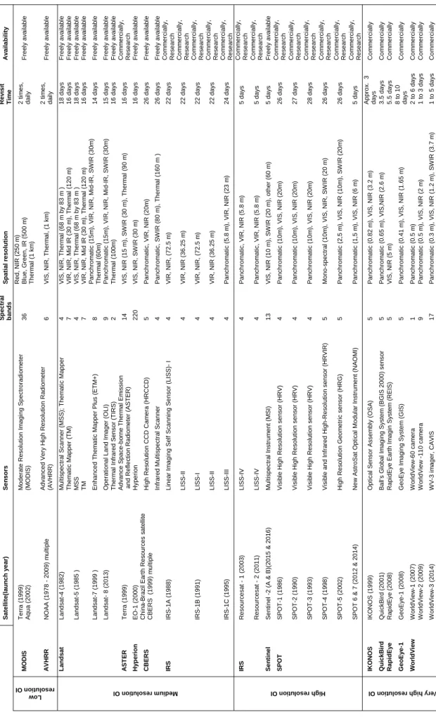
There are approximately 1 381 operating satellites in orbit, of which roughly 344 satellites (including 152 optical imaging satellites) are used for earth observation (UCS 2016). From this list, there are a select few platforms that distribute optical imagery freely, commercially or for research purposes. Popular sources of optical imagery are listed in Table 2.1, together with relevant information regarding their spectral, spatial and temporal resolutions.
2.1.5 Image processing and interpretation
Specialized knowledge of and experience with image interpretation is required to extract useful information from remotely sensed data. Campbell (2007) suggests that there are three different levels of knowledge required for capable image interpretation. First, knowledge of the subject of interest is needed. The subject is the motivation for image interpretation and a sufficient knowledge is required to understand what the imagery is portraying. Second, the location of the study can be equally important given that each area has unique characteristics that influence patterns (tones and textures) on an image. Third, the type of remote sensing system is important, since each remote sensing system has a unique blend of resolution characteristics (spatial, spectral, temporal and radiometric resolutions). Therefore, knowing how these characteristics influence the ability to derive useful information about the subject of interest is essential.
Table 2.1 Popular sources of optical imagery (OI) and their characteristics S at el li te (l au n ch y ear ) S en so rs S p ect ral ba n ds S p a tia l r e s o lu tio n R e v is it T ime A v a ila b ilit y Low re sol ution O I M O D IS T er ra ( 19 99) A qua ( 2002 ) M oder at e R es o lut io n I m agi ng S pec tr or ad iom et er (M OD IS ) 36 R ed, N IR ( 250 m ) B lue, G reen, I R ( 500 m ) T her m al ( 1 k m ) 2 ti m e s , dai ly F ree ly av ai lab le A V HRR N O A A ( 1978 - 20 09) m ul ti p le A dv anc ed V er y H igh R es ol ut ion R ad iom et er (A V HRR) 6 V IS , N IR , T h e rm a l, ( 1 k m ) 2 ti m e s , dai ly F ree ly av ai lab le Me dium re sol utio n OI L an d sat Lands at -4 ( 19 82) M ul ti s pec tr a l S c an ner ( M S S ); T hem at ic M apper 4 V IS , N IR , T her m al ( 68 m by 83 m ) 18 day s F ree ly av ai lab le T hem at ic M apper ( T M ) 7 V IR , N IR , M id I R ( 30 m ), T he rm al ( 120 m ) 16 day s F ree ly av ai lab le Lands at -5 ( 19 85 ) MS S 4 V IS , N IR , T her m al ( 68 m by 83 m ) 18 day s F ree ly av ai lab le TM 7 V IR , N IR , M id I R ( 30 m ), T he rm al ( 120 m ) 16 day s F ree ly av ai lab le Lands at -7 ( 19 99 ) E nhanc ed T hem at ic M apper P lus ( E T M + ) 8 P anc hr om at ic ( 15m ), V IR , N IR , M id -IR , S W IR ( 3 0 m ) T her m al ( 60m ) 14 day s F ree ly av ai lab le Lands at - 8 ( 2 013) O per at ion al Land Im ager ( O LI ) 9 P anc hr om at ic ( 15m ), V IR , N IR , M id -IR , S W IR ( 3 0 m ) 15 day s F ree ly av ai lab le T her m al I nf rar ed S e ns or ( T IR S ) 2 T her m al ( 10 0m ) 16 day s F ree ly av ai lab le A ST ER T er ra ( 19 99) A dv anc e S pac e -bo rne T her m al E m is s ion and R ef lec ti on R ad iom et er ( A S T E R ) 14 V IS , N IR ( 15 m ), S W IR ( 3 0 m ), T her m al ( 90 m ) 16 day s Co m m e rc ia lly , R es ear c h H y pe ri on EO -1 ( 200 0) H y per ion 220 V IS , N IR , S W IR ( 3 0 m ) 16 day s F ree ly av ai lab le CBE RS C hi na -B raz il E ar th R es our c es s at e lli te C B E R S ( 1999) m ul ti p le Hi g h Re s o lu ti o n CCD Ca m e ra ( HRCCD) 5 P anc hr om at ic , V IR , N IR ( 20m ) 26 day s F re el y av ai lab le Inf rar e d M ul ti s p ec tr a l S c ann er 4 P anc hr om at ic , S W IR ( 80 m ), T her m al ( 160 m ) 26 day s F ree ly av ai lab le IR S IRS -1A ( 1988) Li ne ar I m agi ng S e lf S c ann ing S ens or ( LI S S I 4 V IR , N IR , ( 7 2 .5 m ) 22 day s Co m m e rc ia lly , R es ear c h L ISS -II 4 V IR , N IR ( 36. 25 m ) 22 day s Co m m e rc ia lly , R es ear c h IRS -1B ( 1991) L ISS -I 4 V IR , N IR , ( 7 2 .5 m ) 22 day s Co m m e rc ia lly , R es ear c h L ISS -II 4 V IR , N IR ( 3 6 .2 5 m ) 22 day s Co m m e rc ia lly , R es ear c h IRS -1C ( 1995 ) L ISS -III 4 P anc hr om at ic ( 5. 8 m ), V IR , N IR ( 23 m ) 24 day s Co m m e rc ia lly , R es ear c h High re sol ution O I IR S R es our c es at 1 ( 2003 ) L ISS -IV 4 P anc hr om at ic , V IR , N IR ( 5. 8 m ) 5 day s Co m m e rc ia lly , R es ear c h R es our c es at 2 ( 2011 ) L ISS -IV 4 P anc hr om at ic , V IR , N IR ( 5. 8 m ) 5 day s Co m m e rc ia lly , R es ear c h S e nt ine l S ent ine l -2 ( A & B )( 2 015 & 201 6) M ul ti s pec tr a l I ns tr um ent ( M S I) 13 V IS , N IR ( 1 0 m ), S W IR ( 2 0 m ), o th e r ( 6 0 m ) 5 day s F ree ly av ai lab le SPO T SPO T -1 ( 198 6) V is ib le H igh R es o lu ti on s ens o r ( H R V ) 4 P anc hr om at ic ( 10m ), V IS , N IR ( 20m ) 26 day s Co m m e rc ia lly , R es ear c h SPO T -2 ( 199 0) V is ib le H igh R es o lu ti on s ens o r ( H R V ) 4 P anc hr om at ic ( 10m ), V IS , N IR ( 20m ) 27 day s Co m m e rc ia lly , R es ear c h SPO T -3 ( 199 3) V is ib le H igh R es o lu ti on s ens o r ( H R V ) 4 P anc hr om at ic ( 10m ), V IS , N IR ( 20m ) 28 day s Co m m e rc ia lly , R es ear c h SPO T -4 ( 199 8) V is ib le and Inf ra red H igh -R es o lut ion s ens o r ( H R V IR ) 5 M ono -s p e c tr a l (1 0 m ), V IS , N IR , S W IR ( 2 0 m ) 26 day s Co m m e rc ia lly , R es ear c h SPO T -5 ( 200 2) H igh R es ol ut ion G e om et ri c s ens or ( H R G ) 5 P anc hr om at ic ( 2, 5 m ), V IS , N IR ( 10m ), S W IR ( 20m ) 26 day s Co m m e rc ia lly , R es ear c h S P O T 6 & 7 ( 2012 & 2014) N ew A s tr oS at O pt ic a l M odu lar I ns tr um ent ( N A O M I) P anc hr om at ic ( 1, 5 m ), V IS , N IR ( 6 m ) 5 day s Co m m e rc ia lly , R es ear c h Ve ry high r es olu tio n OI IKO NO S IK O N O S ( 1999) O p ti ca l S e n so r A sse m b ly ( O S A ) 5 P anc hr om at ic ( 0. 82 m ), V IS , N IR ( 3. 2 m ) A ppr ox . 3 day s Co m m e rc ia lly Qu ic k B ir d Q ui c k B ir d ( 2001 ) B al l's G lo ba l I m agi ng S y s tem ( B G IS 2000) s e ns or 5 P anc hr om at ic ( 0. 65 m ), V IS ,N IR ( 2. 6 m ) 3. 5 day s Co m m e rc ia lly R a pi dE y e R api dE y e ( 2008 ) R api dE y e E ar th I m agi n S y s tem ( R E IS ) 5 V IS , N IR ( 5 m ) 5. 5 day s Co m m e rc ia lly G e o E ye -1 G eoE y e -1 ( 2008) G eoE y e I m agi ng S y s tem ( G IS ) 5 P anc hr om at ic ( 0. 41 m ), V IS , N IR ( 1. 65 m ) 8 t o 10 day s Co m m e rc ia lly W o rld V ie w W o rl dV iew -1 ( 20 07) W o rl dV iew -60 c am er a 1 P anc hr om at ic ( 0. 5 m ) 2 t o 6 day s Co m m e rc ia lly W o rl dV iew -2 ( 20 09) W o rl dV iew -110 c am er a 9 P anc hr om at ic ( 0. 5 m ), V IS , N IR ( 2 m ) 1 t o 3 day s Co m m e rc ia lly W o rl dV iew -3 ( 20 14) WV -3 i m ager , C A V IS 17 P anc hr om at ic ( 0. 3 m ), V IS , N IR ( 1. 2 m ), S W IR ( 3. 7 m ) 1 to 5 day s Co m m e rc ia lly
2.1.5.1 Image pre-processing
Due to radiometric (measuring electromagnetic energy) and geometric (shape, size and relative position of objects) distortions, satellite imagery has to undergo a rigorous pre-processing phase prior to interpretation and analysis. The rectification and restoration of the acquired imagery are necessary for both spatial and spectral comparisons.
Geometric distortions can be caused by various factors such as oblique viewing distortions (objects in the foreground appear larger than objects farther away), relief displacement and displacement effects caused by the rotation of the earth and satellite sensors’ scan speed (Chuvieco & Huete 2010; Tempfli et al. 2009). These geometric distortions occur either systematically (predictably) or randomly, and are dealt with accordingly. Predictable errors (e.g. the movement of the earth) are better understood and can be corrected by applying mathematically derived formulas. Remaining random distortions are corrected by comparing the distorted image to known, well-distributed ground control points (GCP’s). Least squares regression, used to determine coefficients for two coordinate transformation equations, interrelates the geometrically correct coordinates and the distorted image coordinates (Lillesand, Kiefer & Chipman 2004). Resampling then occurs during which the image is essentially warped to accurately fit the ground coordinates. The preferred approach for image resampling for scientific analysis is the nearest neighbour approach, mainly because it is computationally simplistic and the original input pixel values are not compromised. Other resampling methods include bilinear interpolation and cubic convolution, which are more appropriate for continuous variables and display purposes. The quality of the geometric correction is largely attributed to the selected GCP’s and is a process that generally requires human input (Chuvieco & Huete 2010; PCI Geomatics 2014).
Similar to geometric distortions, radiometric effects are highly variable and sensor-specific. Main causes of radiometric distortions are the deterioration of the sensor’s general performance, discrepancies due to the earth-sun distance and distortions due to the atmospheric effects on EM reflectance (e.g. haze). T