1
Modelling the Distribution of Returns to Higher Education:
A Microsimulation Approach*
Pierre Courtioux Edhec Business School [email protected]
Stéphane Gregoir Edhec Business School [email protected]
Dede Houeto
PSE-Paris School of Economics [email protected]
Abstract
Cost-sharing policy for higher education has been implemented in several countries with various modalities. We argue that to assess their appropriateness and facilitate their implementation it is necessary to develop statistical indicators of the distribution of returns. When starting a higher education programme, the return on a particular degree is uncertain and risk-adverse students or those from a low-income family may be reluctant to enrol. These statistical indicators would therefore be natural inputs of cost-sharing policies intended to preserve the individual economic incentives to go to university and simultaneously providing an insurance role. We present a dynamic microsimulation model of individual lifetime educational output on the French labour market which uses econometric modelling of individual wages, labour market transitions, social security contributions and benefits. It relies largely on labour force survey data and mortality tables. In the standard internal rate of return framework, the model is used to compute the distribution of returns to higher education for a given generation. The results show that the percentage of negative returns is relatively high and close to 7.5%.
Keywords: Return to education; Higher education; Dynamic microsimulation JEL classification: C6, J11, J24
*The estimation of the microsimulation model introduced in this paper was carried out with three sets of data: the French Labour Force Survey for 2003-2007available online (http://www.insee.fr), the French Labour Force Survey 1968-2002, to which access was provided by the Quetelet Centre (http://www.centre.quetelet.cnrs.fr/), and the mortality rates and their forecasts based on Vallin and Meslé (2001) and Robert-Bobée and Monteil (2005). Dede Houeto benefited from EDHEC Business School funding for this research work. The authors wish to thank the anonymous referees for comments that helped us to improve this article.
2
1. Introduction
In terms of public policies, investing in education is one of the key issues for developed countries. The European Lisbon Strategy and its educational part, the so-called ‘Education and Training 2010’, emphasize the link between the education system and social cohesion and establish educational targets such as numbers of early school leavers or an increase in the proportion of Master of Science and Technology graduates (Commission of the European Communities, 2005). Most of these objectives have been maintained and complemented in the new guidelines
issued in 2010 in EU 2020 (Commission of the European Communities, 2010). More
generally, a benchmarking process of the education organization and outcomes in developed countries is in progress (OECD, 2008). It relies on a set of national indicators such as the mean return to higher education. In this article, we illustrate how a microsimulation approach to education outcomes can enhance the issue by means of relatively straightforward modelling. We present a dynamic microsimulation model of educational output for France based mainly on Labour Force Survey data and mortality tables—for a presentation of the French education system see for instance Givord and Goux (2007). We show how it could complement the OECD (2003, 2008) indicator of the mean return to higher education by producing an indicator of higher education valuation risk. For every country, the OECD indicator shows that returns to higher education are largely above the interest rate; this is generally interpreted as an argument in favour of developing a cost-sharing policy. For countries where higher education costs are largely subsidized, this leads to the recommendation of an increase in the student contribution to the training costs without taking into account the possibly large variability of these returns. In this context, our modelling strategy focuses on the risks associated to these returns which should also be taken into account in the design of cost-sharing schemes to promote a sound higher education policy.
The paper is organized as follows: in Section 2, we introduce and discuss the higher education internal rate of return framework for the individuals of a given generation; in Section 3, we detail the microsimulation modelling; in Section 4, we present and discuss the results for our indicator of higher education valuation risk; Section 5 concludes.
3
2. A distribution perspective on higher education returns
According to the classical approach of education economics, education can be considered as an input of human capital that impacts on earnings over the course of a lifetime. The gains of such an investment are usually assessed by computing the individual internal rate of return of one additional year of education. Since the seminal work of Mincer (1974), measuring the internal rate of return to education has become a key dimension of the analysis of education choices—see also Heckman et al., (2006). More recently, the introduction of uncertainty in the dynamic modelling of education choices put the stress on analysing the distribution of returns. For instance in the model of Buchinsky and Leslie (2010) the schooling choice is determined by integrating over uncertain future outcomes, including wages which depend on the individual level of education and experience: they assume that the agent has access to estimates of past wage distributions from which they forecast future distributions in order to make their education choice. As their model is partially estimated and partially calibrated, they can test the impact of the level of unobserved heterogeneity on the individual outcomes. They show that the introduction of unobserved heterogeneity can play a major role in one’s educational choices and consequently in wage outcomes.
Our research explores the idea that a substantial part of this heterogeneity stems from the education system and that this heterogeneity is linked to the heterogeneity of the education services the students benefited. As reported by Altonji et al. (2012), there are few works assessing why individuals choose different types of education and the career consequences of these choices.
In this perspective, our research aims at illustrating how the heterogeneity of education services in terms of subsidies and costs may impact the distribution of internal rates of return to higher education.
From an empirical point of view, such a perspective is demanding, as it requires to work on some long panel data—for instance as in Guvenen (2009)—with variables including diploma obtained and trajectories on the labour market. Such datasets are rarely available. In France, the DEPP (National department of education evaluation) panel data is available for some recent generations—the individuals who completed a secondary education in 1996 and 2001. This panel only allows for a modelling of
4
the first years of a career. This is the reason why we use a microsimulation modelling to produce under some conservative assumptions long panel data for a given cohort with such variables. Based on this cohort, we compute a distribution of internal rate of returns to higher education that is discussed in section 4. The simulation of the cohort analyzed is obtained by combining estimation and calibration—see section 3 for a more detailed presentation of the modelling strategy.
In this view based on past observations, we analyse the distribution of ex ante returns in a framework of choices with uncertainty on the returns. Four assumptions are necessary to interpret our results as ex ante distribution.
1) There is uncertainty for the realization of future wages offered to the individual from a known future wage career distribution; this distribution is conditional on the diploma obtained but could also be analysed by gender or the two-digit sectors of economic activity of a career.
2) The student is not aware of his/her own talent/preferences to study and work. 3) The education decision does not concern a marginal schooling year but rather
an education track which leads to a diploma.
4) The individual decision of pursuing higher education is taken at the age when the student could legally enter the labour force. This decision is irreversible.
As explained earlier the assumption 1 has become a key feature to analyze education choices—Bushinsky and Leslie (2010). The assumption 3 is not commonly used in education economics: this is partly due to the difficulty of estimating structural dynamic model of education choice but this is a promising research agenda in education economics—see Altonji et al. (2012) for a discussion. Moreover, this assumption is more in line with the institutional features of the French education system than the schooling year approach used in numerous studies—for a presentation of the French higher education system see for instance Courtioux (2010)—and could lead to more clear-cut policy recommendation concerning the different segments of the education system. The assumption 4 is clearly a simplification of a more complex decision-making process which is by nature sequential and leads to partial irreversibility for some decisions concerning the investment in human capital—see Altonji et al. (2012) for a discussion. In this view, the results presented in the article correspond to an extreme case: the irreversibility
5
of education choices is total and occurs at the entrance of the tertiary education system. In a dynamic modelling of choices, the results we present also corresponds to the distribution of ex ante returns for the first sequence of individual choice for education—i.e. when s/he could enter the labour force and has a whole uncertainty on his/her tertiary education success potentials. In further researches the impact of these assumptions on our results should be more specifically analyzed. An interesting complement will be to compute a distribution of returns for every year of schooling choice, conditional on the diploma already obtained. Such a development needs data on the individual educational trajectories which are not used in the analysis we propose here.
However, at this stage it is noteworthy that the assumption 2, 3 and 4 are also implicitly made in the construction of OECD (2008) indicators of returns to higher education. However, the OECD’s methodology does not take into account the uncertainty linked to the realization of future wages conditional to the diploma obtained. In this view, the results we propose for France are innovative and complement the previously available OECD benchmark.
To produce a large set of individual histories for a given cohort, we use microsimulation techniques. The microsimulation approach has been used to analyse various issues in economics, notably welfare reforms (Arntz et al., 2008), corporate tax system (Creedy and Gemmel, 2009) or to complete computable general equilibrium models—see for instance Magnani and Mercenier (2009), Mabugu and Chitiga (2009). From an education economics perspective, microsimulation modelling has to tackle two sets of problems. On the one hand, it has to capture the dynamics of individual trajectories in a given socio-fiscal regime. Such problems are traditionally addressed by dynamic microsimulation techniques—see for instance Harding (1993), Nelissen (1998) van Sonsbeek (2010), van Sonsbeek and Ablas (2012). On the other hand, it has to take into account as precisely as possible educational heterogeneity in terms of schooling years and diploma types as well as their economic counterpart on the labour market in terms of employment trajectories, direct wages, unemployment benefits and retirement pensions.
Working with a simulated cohort, we can compute the distribution of internal rate of returns to tertiary educated individuals. Following the human capital approach initiated by Becker (1962), the internal rate of return is obtained by equating the present value of the stream of income when one invests in human capital to its
6
present value when one does not. If X is the stream of income when an agent pursues higher education and therefore enters the job market later and Y is the stream of income when s/he does not pursue higher education and thus enters the job market, the internal rate of return of this individual (r) solves the following equation:
( )
1 0 0 1 = + −∑
= + T t t t t r X Y (1)where t is a time period index and T is the total number of period units lived by the individual.
We look for a representative measure of returns to higher education consecutive to the uncertainty of future wages offered to the individual. We have to decompose the stream of incomes of people in both situations. If we first consider the labour market outputs related to higher education Yt can be decomposed into five components as
follows: t t t t t t
W
U
R
T
F
Y
=
+
+
−
−
(2)where Wt is the individual net wage at period t, Ut the unemployment benefit, Rt the
retirement pension, Tt the individual income tax and Ft the fees. For a given point in
time, some of the elements which compose the labour market outputs may be equal to zero. For instance, the fees (Ft) are positive during the tertiary education period
and equal to zero afterwards. If the individual is employed during period t, the unemployment benefit (Ut) is equal to zero. If the individual is not retired during
period t, the retirement pension (Rt ) is equal to zero. When one considers the course
of a lifetime, the components of Yt are not independent: the level of pension and of
unemployment benefit are linked to the past wage trajectories. In our modelling we analyze these links with the tax benefit component of our microsimulation model— see section 3.2.
We work on the assumption that the counterfactual stream of income obtained when not pursuing tertiary education can be estimated by the average earnings by age for the individuals who did not obtain a higher education degree.1 This assumption is consistent with the education choice framework we presented above. Their earnings are thus defined as follows:
1
We decided not to retain a gender-specific counterfactual, in order to produce a set of return indicators which were not biased by the fact that the individual behaviour vis-à-vis the labour market could be determined by a joint decision within the household.
7 N F T R U W X N i i t i t i t i t i t t ) ( 1 , , , , ,
∑
= − − + + = (3)where N is the number of individuals without a tertiary diploma within the given generation, and Xt is the average net income for a given generation at the age
corresponding to the period t for the individuals without tertiary diploma, weighted by the probability of being employed at this age. The individual stream of income of individuals who have invested in higher education therefore constitutes a way of assessing the distribution of returns to higher education associated with a particular degree. However, a given diploma can itself be related to particular sets of characteristics in terms of skills and social position which are not captured in the reference counterfactual stream of incomes when no degree has been completed. This unobserved heterogeneity may have an impact on the ex post rate of return to higher education—i.e. the realization of individual wage career. In the framework introduced above, this computation is consistent with the assumption that the student’s knowledge about his/her talents is weak. It does not take into account the influence of the signal associated to a degree that may reduce the correlation between the professional talents and academic skills.
Consistently with our non-sequential analytical framework of higher education choice, there is a large variety of opportunity costs for higher education training that the computation resulting from equation (3) does not take into account. Indeed, some students follow a tertiary curriculum for only two years and then enter the labour market at a substantial wage premium, whereas others choose to follow a longer curriculum and therefore face higher opportunity costs: they have already attained a certain level in tertiary education which is associated with higher wages but they prefer to postpone their entry into the labour force. Moreover, some individuals who already have a degree pursue their studies to obtain a higher level degree, but may fail their exam; they then enter the labour force at a greater age with higher opportunity costs than the average for individuals with the same degree level. To capture this variety in higher education investment that have an impact on the level of returns, we compute a particular version of Xt during the education period of the
lifetime for each level of tertiary education (e) already attained by each person. Here,
e stands for the degree level and can be ordered—it corresponds to a partition of
8 t t t t t e W U R T X , = 0, + 0, + 0, − 0, if L≤t (4.1)
}
{
t t et t e MAX X X X X , = 0, , 1,,..., , if L>t (4.2)where L is the period unit at which the individual in our simulated cohort enters the labour force. In this framework, two individuals with the same diploma entering the labour force at different ages (L) support different opportunity costs. The one who enters the labour force the later supports the additional Xt corresponding to the delay
period. Moreover, the opportunity cost estimation is specific for the period of study (equation 4.2). This means that for a given diploma, the opportunity costs are increasing with age (t): they take into account the experience premium on wages of those who enter early the labour force and the education premium of those who have got their degree and are on the labour market—whatever their position—at this given age t. For instance, the opportunity cost of a five-year degree entering very lately the labour force is estimated by the income level of the five-year degrees already in the labour force under the condition that the average income of that class of education level is the highest for this age—i.e. at the very end of his/her studies’ period.
In this framework, a negative individual internal rate of return to education remains possible for educated people: it means that the individual gains associated with his/her highest degree are not sufficient to cover the losses associated with the training years so that the present value of his/her stream of income remains less than that of the average career of those who do not complete a tertiary diploma.
3. A dynamic microsimulation model for France
Our modelling simulates age effect conditionally to diploma obtained. The specification of our microsimulation model is constrained by data available. We have at our disposal the French Labour Force Survey (FLFS) for the period 1968-2007. However, the data collection method was changed in 2003. One of these changes concerns the education variable: this variable is now more detailed. We want to use as far as possible the FLFS 2003-2007 to capture the effect of diploma at a level disaggregated as much as possible. In this view, FLFS 2003-2007 is used to define the determinant of wages conditionally on the diploma obtained. It is also used to identify the relative probability of transition on the labour market conditionally on the diploma obtained. This leads us to focus on the simulation of a generation mainly on
9
the labour force during the 2003-2007’s period in order to have smaller cohort effect bias in our simulation. We choose to focus on the generation born in 1970.
However, the 2003-2007’s period is too short to capture date effects such as the impact of business cycle on employment, experiences and wages at a disaggregated diploma level. Our modelling strategy aims at controlling the business cycle effect on individual trajectories by estimating a chronogram of situation on the labour market conditionally to current unemployment rate. This chronogram is estimated on the FLFS 1968-2007. In the microsimulation, the chronogram is used to calibrate the destiny of a whole generation, whereas the wage modelling and the transition on the labour market modelling are used to simulate conditional on their degree individual trajectories under this generational constraint. This means that we assume that we can forecast the chronogram of a generation based on the observed former generation. Doing so, we potentially miss some cohort effects mainly effective at the end of the career, linked for instance to the raise of retirement age in France. Additional simulations have confirmed that the consequences of disregarding these cohort effects are small.2
The dynamic microsimulation model used to simulate the careers of a generation has a specification that can be decomposed into three basic operations: (1) a simulation of the individual transitions on the labour market, (2) a simulation of individual earnings, and (3) a simulation of mortality rates over the course of a lifetime. At each level, we explicitly take into account the heterogeneity deriving from the type of tertiary diploma obtained.
3.1. Modelling transitions on the labour market over the lifecycle
In order to estimate the distribution of returns to higher education, we are interested in modelling the transitions on the labour market for a given generation over its lifetime. Because of the characteristics of the French socio-fiscal regime—notably the existence of specific careers for public employees (fonctionnaires) which are entitled for instance to particular rights concerning retirement pensions—we have to model the transitions between five states: (1) inactivity, (2) self-employment, (3) public employment, (4) other private employment, (5) unemployment, but want to keep the
2
We tested the effect of an extension of high employment years and a consecutive delay on retirement ages. It has a small impact on our results, mainly because the internal rate of return is principally impacted by the years at the beginning of the life cycle.
10
random simulation of these transitions under control by imposing an overall constraint on the implicit distribution of a generation over the different states that is consistent with the observed labour force participation rate.
To model the individual transitions on the labour market over the lifecycle, we assume that Pi,t , the probability for an individual i to be in a given state at the t
period, is a function of some invariant individual characteristics—gender and diploma— of the macroeconomic conditions—notably the level of unemployment— and the past trajectory of the individual. This can be illustrated by the following equation where mi is the gender of the individual i, ei the education characteristics, and Ut the current unemployment rate:
) ,..., , , , , , ( , ,( 1) ,( 2) ,( ) ,t i i it t i t i t i t t i f m e a U P P P P = − − − (5)
Our modelling strategy consists of two steps: we first estimate general aggregated patterns of the positions on the labour market for a generation across the ageing process. The dependent variables are the labour force participation rate, the unemployment rate and the self-employment rate at a given age and time period; we then estimate individual differentials in transition probability for individuals in the light of their education and their past trajectories. The simulation of transition consists of a random draw based on an individual probability differential which is aligned with the age-specific aggregated rate of the first step3.
In this very first step, we posit a model to capture the mean pattern of activity over the lifecycle for a given generation. The mean pattern of the three aggregated rates (P) at the period t for a given generation is supposed to be a function of gender (m), age of the generation during the current period (at) and the current situation of the
labour market captured by the current unemployment rate (Ut):
)
,
,
(
t t tf
m
a
U
P
=
(6)We therefore assume that this age-specific pattern at a given point of time corresponds to the combination of the rates associated with five labour market positions: (1) labour force participation rate, (2) unemployment rate, (3) self-employment rate, (4) public self-employment rate, and (5) other private self-employment rate. We model the various aggregated rates associated with (1), (2), (3) and for the sake of simplicity assume that the public employment rate (4) is not age-specific and
3
11
corresponds to the one observed during the 1968-2005 period in France (i.e. 20% of employment). The indicator (5) is then computed as the remainder.
The specification of the indicator modelling equation corresponds to the use of a polynomial approximation in the age variable (t - g). Technically the following model is estimated separately for men and for women to account for their specific activity patterns during the life course:
ε
φ
ϕ
δ
χ
β
α
+ − + − + − + − + + − + + + = − t g x t g t g D U g t g t g t g t g t P P ) ( ... ) ( ) ( ) ( ) ( ) 1 log( 2 3 4 , , (7) where Pg,t is the indicator associated with generation g at the period t that can takethree values: respectively the rate of labour force participation, the unemployment rate, and the self-employment rate and Ut the current unemployment rate, whereas
Dg is a generation dummy. The model is estimated from the segments of generation
patterns computable from the FLFS 1968-2005. For instance, the generation born in 1950 is observed from age 18 to 55; the generation born in 1951 is observed from age 17 to 54, etc. The different orders of the polynomial approximation are tested. The final estimation only retains the orders that are significant. The results of this final estimation are reproduced in Table 1.
Table 1
Estimates of the age-specific activity pattern modelling
men women men women men women
α -21.25 * -27.11 * 3.53 * 3.25 * -6.47 * -7.115 * β 1.75 * 2.74 * -0.56 * -0.43 * 0.28 * 0.31 * χ -0.04 * -0.10 * 0.01 * 0.01 * -0.01 * -0.01 * δ 0.00042 * 0.00153 * -0.00010 * -0.00007 * 0.000006 * 0.000006 * φ -0.000002 * -0.000001 * Ut -3.44 * -3.44 * 0.26 * -3.44 * 0.55ns 1.30ns R-square 0.97 0.92 0.82 0.82 0.94 0.90 LFP U SE estimates
Source: French Labour Force Survey 1968-2005 (Insee, 1999); authors’ calculations.
Note: Taking 1970 as a reference, this model is estimated with dummies for each generation which are not reproduced here. LFP: Labour force participation, U: unemployment, SE: self-employment. (*) significant at 1%, (ns), non-significant.
Knowing the aggregated age-specific levels of activity pattern of a given generation for the current macroeconomic conditions we can turn to the modelling of the differential in the probability of transition across lifetime for the individuals of a given
12
generation. As noted above, we assume that this differential can be characterized by the education level and the past individual labour market history. Several approaches can be used to model the transitions between the five states introduced above. For instance, a multinomial logit model could be considered. Adopting a practical perspective, we follow the approach that has been used with success in another French microsimulation model (Destinie) developed by Insee—see Insee (1999), Blanchet and Le Minez (2009). This approach moreover facilitates the alignment process during the simulation. We estimate a set of sequential binomial logit models with the FLFS 2003-2005 rather than a multinomial logit model. They correspond to the sequence of binary decompositions of the labour market positions. We first model the probability conditional on the past labour market position and the education level; second, P (li,t= 1) of being in the labour force at the period t denoted by li,t =1, P (oi,t=
1 | li,t = 1) where oi,t is a dummy variable equal to one when the individual is
self-employed at the period t; third, P (qi,t= 1 | li,t = 1 and oi,t = 0) where qi,t is a dummy
variable equal to one when s/he is employed in the public sector at the period t; and fourth, P (ri,t= 1 | li,t= 1 and oi,t= 0 and qi,t= 0) where ri,t is a dummy variable equal to
one when s/he is employed in the private sector at the t period. The equations estimated are of the following form:
i t i t i t i P C e Z, =
α
. ,(−1)+β
. ,(−1)+δ
. (8)where Zi,t is a latent variable corresponding to the four conditional probabilities
previously specified, Pi,(t-1) is a variable stating the status vis-à-vis the labour market
the previous year, and Ci,(t-1) is a matrix of cumulative indicators of the past individual
trajectories, namely years of experience—the difference between current age and age when entering the labour force used as a proxy variable—, the time spent out of the labour force, a dummy for long-term unemployment, and ei as the education
level—a diploma variable broken down into 20 items which are detailed in the Appendix (Table A1, specification 1). The estimates are given in Table 2.
13
Table 2
The determinants of the individual position on the labour market (logit)
(A) (B) (C) (D) ref. -5.438 * -5.336 * -1.834 * 2.489 * -6.610 * -6.341 * -3.091 * 5.057 * ref. -5.555 * -1.834 * 4.166 * -10.020 * ref. -1.874 * 3.784 * -8.122 * -6.326 * ref. -0.018 * 0.040 * 0.067 * 0.045 * -0.00003 * -0.001 * -0.001 * -0.365 * -13.459 ** -16.551 *
no diploma (ea) ref. ref. ref. ref.
CAP/BEP (eb) 0.354 * -0.054 * 0.553 * 0.300 *
bac (general) (ec) 0.262 * 0.359 * 0.500 * 0.337 *
bac (profesionnal) (ed) 0.914 * 0.295 * 0.083 * 0.653 *
bac (technical) (ee) 0.495 * 0.056 * 0.593 * 0.451 *
capacité en droit (ef) 0.934 * 0.163 ** -0.841 * -0.396 *
DEUG (university two-year degrees) (eg) 0.078 * 1.036 * 0.470 * 0.124 *
DUT/DEUST (university two-year degrees) (eh) 0.772 * -0.285 * 0.275 * 0.848 *
BTS (two-year degrees) (ei) 0.617 * 0.471 * 0.008 ns 0.681 *
other higher technician (two-year degrees) (ej) 0.068 * 0.691 * 0.110 * -0.042 *
paramedical (two-year degrees) (ek) 0.376 * 2.421 * 3.606 * 1.121 *
licence (university three-year degrees) (el) 0.139 * 0.576 * 1.212 * 0.272 *
other three-year degrees (em) 0.739 * 0.905 * 0.302 * 0.623 *
maîtrise ( university four-year degrees) (en) 0.314 * 0.637 * 0.844 * 0.202 *
DEA (university five-years degrees) (eo) 0.511 * 0.242 * 0.826 * 0.190 *
DESS (university five-year degrees) (ep) 0.859 * -0.112 * 0.429 * 0.391 *
business schools (five-year degrees) (eq) 1.164 * -0.464 * -0.626 * 0.529 *
engineering schools (five-year degrees) (er) 0.827 * 0.671 * 0.151 * 0.634 *
Ph.D (medical degree excluded) (es) 0.935 * 0.344 * 1.362 * 0.422 *
Ph.D (medical degree) (et) 0.694 * 0.796 * 3.223 * 1.205 * 0.955 0.958 0.911 0.720 97.7 97.6 95.2 85.6 2.2 1.9 4.2 13.5 0.1 0.5 0.6 0.9 long-term unemployment α inactive (t -1) unemployment (t- 1) self-employment (t -1) public employment (t -1) other private employment (t -1)
β
experience (in years) experience (square)
time out of the labour force (in years)
δ
Sommers'D
percentage concordant percentage discordant percentage tied
Source: French Labour Force Survey 2003-2005 (Insee, 1999); authors’ calculations.
Note: The modelled probabilities are P (li,t = 1) for A, P (oi,t = 1 | li,t = 1) for B, (qi,t = 1 | li,t = 1 and oi,t = 0) for C, P (ri,t = 1 | li,t = 1 and oi,t = 0 and qi,t = 0) for D. To estimate these coefficients, we controlled for gender, number of children for women, the presence of children aged up to three (equations A, B, C and D), several age dummies for age 55 and more, age 60 and more, age 65 and more (equation A); they are not reproduced here.
The simulation of consistent individual transitions over a lifetime replicates the same pattern for each period unit t. It proceeds as follows. First, the individual probability of transition to the position of labour force participation is calculated. This probability is included in the ]0;1[ segment. Then, a random number is drawn from a uniform
14
probability law on the unit segment and multiplied by the individual probability. The individuals are ordered according to this value and the individual status—active versus inactive— is determined by an alignment with the age-specific target associated with the corresponding age. This simulation procedure is consistent with our modelling strategy: it takes explicitly into account the probability differential between individuals with different characteristics. However a given individual has an ex post probability of having been selected in line with his/her estimated probability. The procedure is repeated for self-employment, employment in the public sector and employment in the private sector. The individuals in unemployment are those who have not yet been allocated at the end of the process.
3.2. Modelling earnings
The modelling of earning uses a two-step method. First, the earnings stemming directly from employment are modelled. Second, based on a tax and benefit model corresponding to the current French socio-fiscal regime the indirect earnings stemming from the labour market—unemployment benefit and retirement pension— are computed from the individual trajectories. The net earnings are computed during this second stage: based on the gross earnings, the income tax is calculated.
In line with our analytical framework, our modelling strategy aims at distinguishing the determinants of wages by diploma but we do not try to model the dynamic choice of a curriculum. We work conditionally on a level of education attainment. In this view, this is not possible to use the FLFS 1968-2003. We estimate separately Mincer’s earnings equation by education level and consider the following standard specification: i e i e e s e i e e i e e i e i s e e x x s f w , , , 2 , , , , ) . . . . . log( =α +β +δ +η +µ +ε (8)
where we,s,i is the monthly wage—as available in the FLFS 2003-2007—of individual
i, with diploma e, working in the industrial sector s—the different education and
industrial sector items are listed in Appendix Tables A1 and A2—, and where x is the number of years of experience and f a dummy stating if the individual is a civil servant (fonctionnaire) or not. The sum of the industrial sector effects is constrained to be equal to zero. Moreover, in order to capture the specificity of women’s careers the experience parameter (β) is decomposed into two elements: a mean slope (β1)
15 i e i e i e e x e x e x, 2 , 1 , . . . β β β = + (8.1)
Because of the small number of observations for some diplomas, we have to pool some of them when estimating the equations.
The pooling of some diplomas means our estimate could be affected by some endogeneity bias that one could limit by considering pools of similar levels of education attainment. We consequently use a particular approach to decide which diplomas have to be pooled. The pooling is based on the proximity of diplomas regarding their situation in the labour market. In order to identify this proximity we use a clustering method based on factor analysis whose results are available on request. When the results of the factor analysis are not conclusive, the pooling is based on the proximity of diplomas in terms of education level. Finally, eight earning equations are estimated with six equations concerning higher education diplomas. The results of the estimates are given in Table 3. In the case of pooled estimations, we identify the specific effect of a given diploma in the set of pooled diplomas by a dummy with respect to a reference. In Table 3, the coefficient associated with the reference diploma is α1 and the set of coefficients of the specific dummies associated with the
other diplomas are denoted by α2 crossed with the diploma label.
The exact number of years of experience in employment is not available in the FLFS. As mentioned earlier, however, the difference between current age and age of entry to the labour force is used as a proxy. Nevertheless, to estimate the impact of this variable measured with errors on the wage level, we use an instrumental variable method (IV) on the Mincer equations. Our instruments are: the youth (under 25) unemployment rate, the year of entry to the labour force and a variable describing the family situation differentiated by gender—number of children (1) up to 18 months, (2) between 18 months and three years, (3) between three and six years, (4) between six and 18 years, and (5) a dummy variable for lone parents. To analyse the explanatory power of these instruments, we run an OLS regression of the number of years of experience for each sex. We consider that they are adapted when the coefficient of determination is above 0.35 (R² ≥ 0.35). The last line of Table 3 states the method finally retained for each of the estimations. For the final estimation, we discard the industrial sector variables (η) with non-significant estimates.
16
Table 3
Estimation of wage equations by diploma (monthly wage log in €2005)
ea, eb ed e c , ee, ef, eg e h ei, ej, ek e l , em, en eo, ep, eq, es, t er (A) (B) (C) (D) (E) (F) (G) (H) α1 6.94 * 6.96 * 6.99 * 7.07 * 7.07 * 7.19 * 7.36 * 7.52 * α2 no diploma (ea) -0.08 * CAP/BEP (eb) ref. bac (general) (ec) ref. bac (technical) (ee) -0.04 * capacité en droit (ef) -0.16 * DEUG (university two-year degrees) (eg)
0.11 * BTS (two-year degrees) (ei)
ref. other higher technician (two-year degrees) (ej)
ref. paramedical (two-year degrees) (ek)
0.17 *
licence (university three-year degrees) (el) 0.00 *
other three-year degrees (em)
0.11 * maîtrise ( university four-year degrees) (en)
ref.
DEA (university five-years degrees) (eo) ref.
DESS (university five-year degrees) (ep) ref.
business schools (five-year degrees) (eq)
0.12 *
Ph.D (medical degree excluded) (es) 0.08 *
Ph.D (medical degree) (et) 0.25 *
β1 0.021 * 0.036 * 0.026 * 0.043 * 0.034 * 0.043 * 0.053 * 0.047 *
β2 -0.014 * -0.018 * -0.016 * -0.013 * -0.013 * -0.016 * -0.015 * -0.012 *
δ -0.0002 * -0.0005 * -0.0001 * -0.0005 * -0.0003 * -0.0005 * -0.0008 * -0.0007 *
η
manufacture and construction (sa)
0.05 * 0.06 * 0.06 * 0.07 * 0.08 * 0.07 * 0.19 * 0.07 *
energy (sb)
0.20 * 0.22 * 0.17 * 0.10 * 0.09 * 0.28 * 0.23 * 0.18 *
finance (sc)
0.19 * 0.13 * 0.10 * 0.09 * 0.11 * 0.12 * 0.09 *
services for firms (sd)
-0.03 * 0.01 * 0.07 * 0.02 * 0.04 * 0.08 * 0.07 * services for consumers (se) -0.23 * -0.11 * -0.26 * -0.27 * -0.19 * -0.25 * -0.34 * -0.25 *
administration (sf) -0.17 * -0.13 * -0.08 * -0.07 * -0.09 * -0.18 * -0.15 * -0.24 * other sectors (sg) -0.002 * -0.04 * -0.03 * -0.07 * -0.13 * 0.08 * µ 0.26 * 0.12 * 0.19 * 0.07 * 0.10 * 0.23 * 0.08 * 0.06 * R² 0.37 0.40 0.42 0.53 0.41 0.45 0.47 0.54
Estimation method IV simple IV simple simple IV simple simple
Source: French Labour Force Survey 2003-2005 (Insee, 1999); authors’ calculation.
Note: (*) for 1% level of significance. (A) no diploma and CAP/BEP, (B) bac (professional), (C) bac
(general and technical), capacité en droit and DEUG, (D) DUT/DEUST, (E) other two-year degrees (F) three- and four-year degrees, (G) five-year and more degrees (engineering school excluded), (H) engineering school.
The individual residuals corresponding to the estimates (εi) are stocked and used
during the simulation. At the starting step of the microsimulation, each individual is randomly assigned an observed residual depending on his/her diploma. During the dynamic simulation process, the residual is kept until the individual leaves employment. When s/he finds a new job, a new residual is then randomly assigned. Unfortunately, data on self-employment earnings are not always available in the FLFS or are poorly measured. In the simulation we decided to impute wages as a
17
proxy of self-employment earnings but, being aware of the limitations of such an assumption, we limit the use of the simulation for this category.
The microsimulation takes into account the main features of the French socio-fiscal regime: unemployment benefit, pensions and income tax. According to social legislation, the calculation of workers’ rights to unemployment benefits and pensions is linked to gross wages, which are not available in the FLFS. In line with the current level of social contribution rates, we proxy the gross wages as a fixed share (120%) of net wages.
The unemployment benefit is computed in line with the current legislation: the
Allocation d’aide au retour à l’emploi (ARE). The entitlement and the amount of that
benefit are legally linked to past wages and employment duration. The three main components of the pension system are simulated. The basic pension is obtained by applying the official formula for the 25 best years resulting from the simulation as well as the complementary pensions. Middle ranking and senior executives (cadres) benefit from a specific scheme. Following the common collective labour agreement, we assume that those with a five-year higher education degree or more are cadres. The complementary pensions are based on payroll taxes actually paid throughout a person's career and we use the current rates. The civil servants’ regime is also simulated. It applies to those who have worked for more than 41 years in the public sector; their pension is then a fixed share of their final salary.
The French income tax is not based on individuals but on a particular definition of a household. Theoretically, the tax depends on the number of persons—including children—within the household. In our simulation, we assume that all the individuals are single. This is a simplifying assumption that will limit the interpretation of our results but, in this first step, we do not want to take into account the peculiar influence that the French fiscal system may have on household formation. Further research will be devoted to this analysis because of the possible impact of endogamy related to the education level in our measure. This means that the aggregate revenues of income tax are overestimated inasmuch as they do not take into account the tax cut (dépense fiscale) for family conditions.
18 3.3. Modelling mortality
The existence of a positive correlation between education and life expectancy is well documented and confirmed for France—see for instance Mackenbach et al. (2008) and Menvielle et al. (2007). The pure impact of education on life expectancy is, however, difficult to disentangle from the influence of income and health practice that are correlated with education. When one controls for the effect of these variables the impact of education tends to decrease but remains significant.4 Keeping account of these results, our modelling strategy consists of introducing a weight at the different ages of an individual corresponding to the survival function of their education level. The survival functions are differentiated by sex and education. Our modelling strategy does not take into account the fact that the apparent education/mortality link may result of some selection in tertiary schooling of the healthier individuals whose other characteristics induce better health. We consider that not taking into account this unobserved heterogeneity in our modelling is an acceptable simplification given our analytical framework—i.e. under the assumption of uncertainty of the individual on his/her own talent/preferences for studies.5
In France, mortality tables by education level are not available. Vallin and Meslé (2001) and Robert-Bobée and Monteil (2005), however, give some cross-section mortality tables by socio-economic status. To estimate the mortality tables by diploma for the individual of a given generation, we proceed in two steps. First, we estimate cross-section mortality tables by diploma for the 1991-99 period. Second, we design a method to extrapolate these tables.
Survival functions by level of education
To model mortality differentials, we first compute a mortality table by diploma. We use mortality tables by age, gender and socio-economic status—currently available for France— and the French Labour Force Survey (FLFS) for this computation. Robert-Bobée and Monteil (2005) provided mortality rates for the 1991-99 period. We apply the mortality rates by age, gender and socio-economic status for this period to
4
See for instance Schnittker (2004), Cutler and Lleras-Muney (2006). 5
The modelling does neither take into account the fact that for a given diploma different past trajectories may impact the mortality age—for instance different the level of income. Insofar as the magnitude of this effect is difficult to estimate for econometricians, we consider as an acceptable assumption that this effect does not impact the ex ante distribution of returns to higher education conditioning education choices.
19
the individuals in the FLFS 2003-2005. We then compute the average mortality rate by level of education and age in the FLFS sample. The sample is too small to allow for a robust estimation of highly disaggregated tables by level of education so we aggregate some diplomas. In the aggregation process, we choose to maintain as much as possible a differentiation by education type. For instance, we differentiate high school degrees according to their type—general versus specialized—and we differentiate the higher education diplomas according to their specificity—school system versus university. Finally, we retain eleven diploma classes—the aggregated classes are presented in Appendix Table A1, specification 3.
The data on mortality rates by socio-economic status and the FLFS dataset used do not correspond to the same time period. The mortality tables cover the 1991-99 period, but they are applied to the FLFS 2003-2005 sample. A computation based on the FLFS 1991-1999 sample is possible, but the available diploma variable in these surveys is not disaggregated enough for our analysis. This mismatch in the periods could bias the mortality rates if the relative proportion of various socio-economic groups in the population changed between 1991-99 and 2003-05. To assess this issue, we analyse the repartition of the population into the various socio-economic groups between 1999 and 2003, the last years of the two periods we consider—the tables are available on request. We find that this repartition has not changed significantly. The second step is to model and estimate mortality rates by age and diploma. We posit the following equation for men and women separately:
(9) where: e e
α
1α
2,α
=
+
(9.1) e eβ
1β
2,β
=
+
(9.2) e eγ
1γ
2,γ
=
+
(9.3) e eδ
1δ
2,δ
=
+
(9.4)and Ma stands for the mortality rate at age a, and e for the level of education. The
interaction terms reflect the fact that the impact of the level of education on mortality not only affects the intercept of the mortality curves—the coefficient α, i.e. a
difference in value for each age—but also the slope— the coefficient β, i.e. a difference in the rate of mortality as age increases. This specification is inspired by
2 , , . . 1 log . 1 log a a M M M M e e a a e e e a e a
α
β
+γ
+δ
− + = −20
Insee (1999), but we add interactions with age and age squared to reflect the fact that the impact of the level of education on mortality decreases towards the end of life. This specification is justified by Robert-Bobée and Cadot's (2007) results: they show that although mortality differentials persist in old age, their magnitude decreases. We estimate equation (9) using on the one hand the mortality tables by level of diploma that we computed, and on the other hand the mortality tables by age and sex provided by Vallin and Meslé (2001). The results of our regression are reported in Table 4. This modelling allows for the computation of survival functions.
21
Table 4
Regression of mortality by age on mortality by level of education
variable men women
α1 1.1832 * -1.221 * β1 1.0997 * 0.8383 * γ1 -0.0116 * -0.0053 * δ1 0.0000 ns 0.0002 * α2 CAP/BEP (eb) -0.5125 * -0.3404 * bac (general) (ec) 1.148 * -0.7679 * bac (others) (eD) -0.4375 ns -0.3675 *
two-year degrees (paramedical degree excluded) (eG) -7.6262 * -1.267 *
paramedical (two-year degrees) (ek) 1.2109 * -0.5218 *
three-year degrees (eL) -1.4988 * -0.941 *
four-year degrees (en) 5.1688 * -1.3131 *
university five-years degrees (eO) -2.3255 * 0.0131 ns
business and engineetring schools (five-year degrees) (eQ) -1.3314 * -2.4456 *
Ph.D (eS) 7.1069 * -2.7472 *
β2
CAP/BEP (eb) -0.0363 *** -0.0309 *
bac (general) (ec) 0.0558 ns -0.0799 *
bac (others) (eD) -0.153 * -0.0364 **
two-year degrees (paramedical degree excluded) (eG) -1.0102 * -0.0958 *
paramedical (two-year degrees) (ek) 0.071 ** -0.0267 *
three-year degrees (eL) -0.2511 * -0.0684 *
four-year degrees (en) 0.5859 * -0.106 *
university five-years degrees (eO) -0.3388 * 0.0704 *
business and engineetring schools (five-year degrees) (eQ) -0.1213 ** -0.1822 *
Ph.D (eS) 0.8084 * -0.2468 *
γ2
CAP/BEP (eb) 0.005 * 0.0000 *
bac (general) (ec) -0.0368 * 0.0001 *
bac (others) (eD) -0.0347 * 0.0001 *
two-year degrees (paramedical degree excluded) (eG) 0.0075 ns 0.0001 *
paramedical (two-year degrees) (ek) -0.0435 * 0.0000 ns
three-year degrees (eL) -0.0249 * 0.0001 *
four-year degrees (en) -0.0555 * 0.0001 *
university five-years degrees (eO) -0.0197 * 0.0000 *
business and engineetring schools (five-year degrees) (eQ) -0.0097 * 0.0000 *
Ph.D (eS) -0.0791 * 0.0002 *
δ2
CAP/BEP (eb) 0.0000 ns -0.001 *
bac (general) (ec) 0.0003 * -0.0027 *
bac (others) (eD) 0.0004 * -0.0064 *
two-year degrees (paramedical degree excluded) (eG) 0.0007 * 0.0046 *
paramedical (two-year degrees) (ek) 0.0004 * 0.0002 *
three-year degrees (eL) 0.0004 * 0.0012 *
four-year degrees (en) 0.0001 ** 0.0022 *
university five-years degrees (eO) 0.0004 * 0.0036 *
business and engineetring schools (five-year degrees) (eQ) 0.0002 * 0.0184 *
Ph.D (eS) 0.0001 * 0.0096 *
R² 0.9978 0.9998
Source: FLFS 2003-2005 (Insee), Vallin and Meslé (2001), Robert-Bobée and Monteil (2005); authors’
calculations.
Note: The category of reference for the education variable is ‘No Diploma’; (*) for 1%, (**) for 5% level
22 Extrapolating survival functions
The previous sub-section showed how we estimate mortality differential by diploma at a given point of time. In this subsection, we explain our extrapolation methodology of mortality rate for a given generation which by definition covers several points in time. To illustrate this issue, if one considers the 1970s' generation, one needs the differential in mortality rate in 2000, when the individuals are thirty; for this, we can reasonably use the estimations previously presented—which are for the 2003-04 period—but the mortality rate differential is also needed for each forthcoming year of the period during which an individual born in 1970 is still alive.
Mortality rates have been decreasing in France for the past two and a half centuries (Pison, 2005) and in order to model the average yearly decrease in mortality rate we need the mortality rates for two points in time. Unfortunately the only available mortality rate forecasts are only those by age and gender for 2049—see Vallin and Meslé (2001). We make the assumption that the relative evolution of mortality rates over time is the same regardless of the level of education. We thus apply the average yearly decrease in mortality by age and gender to the mortality rates by education level. This simple hypothesis is conservative and may not be consistent with past observations (Menvielle et al., 2007). Research works in this area are not numerous and owing to lack of information we select this assumption. It is also consistent with our approach since, in the estimation of wages in the microsimulation model, we do not include a change in the wage differential by level/type of diploma. Similarly we do not model any other changes over time that could explain the evolution of the mortality differential, such as differentiated changes in access to health care by education level, for example. This extrapolation assumes that the logarithm of mortality rate decreases linearly as time goes on. This assumption seems reasonable given the fact that the evolution of mortality rates in France has so far been linear (Vallin and Meslé, 2001).
To extrapolate the mortality rate differential throughout the years, we use the midpoint of the available mortality rates in 1991-99 and those computed in 2049 and proceed by linear interpolation, as follows.
(10)
( )
(
)
(
)
(
)
− ∗ − + = 54 ) 1995 ( log ) 2049 ( log 1995 )) 1995 ( log( exp , , a a e a e a M M n M n M23
where Ma,e (n) is the mortality rate by age and level of education for year n. In the
microsimulation exercise, the ageing process is captured by a reduction of the weight associated with each individual: each individual trajectory is simulated from age 16 to age 100 and the specific weight of each individual is corrected by a factor equal to the mortality rate at each age depending on the associated education level. A picture of the survival function obtained by gender and level of education is presented in Appendix Figure A4. As expected, those with the highest levels of education have higher survival rates. However, these differences remain relatively small. Moreover, consistent with the literature, mortality differentials are smaller for women.
4. Results
We now turn to the presentation of the results of the distribution of internal rate of returns to tertiary education for the generation born in 1970 obtained by microsimulation. We take the characteristics—gender, diploma and age of entry to the labour force—of the individuals born between 1968 and 1972 as a representative distribution of the characteristics of that generation. On the basis of the FLFS 2003-2007 we can distinguish 457 weighted classes. For instance, women with a business school degree entering the labour force at 25 constitute one of these classes. From these 457 weighted classes we create 34,782 artificial observations for which we relate randomly an industrial sector based on the empirical distribution by gender and diploma for the individuals under 30 in the FLFS dataset. Then we simulate their life course as explained in section 3. We then compute on this simulated database an internal rate of returns for each individual with a tertiary diploma as explained in section 2 and therefore obtain a distribution of these returns by diploma.
First of all, it is interesting to compare our results with those obtained by OECD (2003, 2008). According to OECD, the mean rate of return to higher education in 1999-2000 is 12.2% for men and 11.7% for women; for 2004 the mean rate of return is 8.4% for men and 7.4% for women. When we apply OECD’s methodology on our simulated panel (only one generation), we obtain a mean rate of return of 12.6%.
24
Table 5
Returns to higher education
education median return part of negative returns All graduates 11.6% 7.5%
DEUG (university two-year degrees) (U2) 6.5% 15.4%
other two-year degrees (S2) 14.3% 6.7%
licence (university three-year degrees) (U3) 7.5% 13.4%
other three-year degrees (S3) 13.5% 4.4%
maîtrise ( university four-year degrees) (U4) 9.0% 9.7%
university five-years degrees (U5) 11.7% 5.3%
other five-year degrees (S5) 15.2% 2.6%
Ph.D (Up) 9.3% 3.8%
Source: authors’ calculations.
Note: the specification of the tertiary diploma is detailed in Appendix Table A1 (specification 4).
The main interest of our methodology, however, lies in the fact that it allows for an analysis of the distribution of returns. First, the median rate of return is equal to 11.6%, which is slightly below the mean—see Table 5. Second, the level and dispersion of returns are not homogeneous. They vary with the curriculum pursued. In France, the highest level of median return is attained for the five-year diplomas obtained in the very selective engineering and business schools (S5), whereas the lowest one is associated with the two-year university degrees (U2) without any professional training. More generally, at the same education level, the diplomas obtained in schools which are selective give a higher median rate of return than the university diploma. When one considers a given system—university versus school— the median rate increases with the number of schooling years, with two exceptions that can be explained by the specificities of the French higher education system. First, the three-year school degree median rate is below the two-year school degree median rate. This is mainly explained by the fact that it corresponds to different types of diplomas. The three-year degrees are marginal in the school system; they represent 1.6% of the generation born in 1970 whereas for instance the more standard vocational short-term tertiary diploma remains the so-called two-year degree BTS (brevet de technicien supérieur) which corresponds to 8.8% of the generation. Second, the PhD degree (Up) exhibits a lower return than the university
25
five-year degree (U5). To interpret these results, one has to keep in mind that in France engineering or business school diplomas are more prestigious than university degrees whatever their level. PhDs are overrepresented in the low-wage sectors for tertiary educated like the administration sector—see Table 3 where η estimates the impact of the different sectors on wages. In the administration sector (sf)—which covers administration, education (higher education and research), health and social services—the part of university five-year degrees is relatively high (34%), whereas it reaches 54% for PhDs. Moreover, holders of a PhD tend to enter the labour force very late. As a consequence, compared with five-year university degrees, the opportunity costs tend to be higher for the marginal training years—see equations (4.1) and (4.2). As an illustration, the mean age of entry to the labour force for PhD degrees (Up) is 28.3, whereas for the five-year degrees it reaches 25.3 for the university degree (U5) and 24.2 for the engineering and business schools (s5).
If we turn now to the dispersion, our results show that the part of educated people in our cohort with negative return is significant and on average reaches 7.5%. This figure can be interpreted as the risk of not benefiting from a tertiary education. It means that 7.5% of tertiary diplomas have a present value of the associated net incomes that is lower than the average present value of net incomes of those who have not completed a tertiary diploma. These negative individual rates can be related to career choices entirely or partially constrained by the institutional framework and the labour market opportunities for the skills gained. These features result from the choices made by employers and employees based on their respective sets of information. From the student’s perspective, they may be explained by imperfect information about the hierarchy of returns across diploma types related to salaries and unemployment exposure or personal knowledge of the ability to complete a tertiary diploma.
Our results suggest that the risk on the value of median return to tertiary education is not homogeneous. It differs across diploma classes. The risk level is consistent with the diploma hierarchy when one considers median rates of return: the lowest risk level amounts to 2.6% for the five-year tertiary school degrees, whereas the highest level amounts to 15.5% for the two-year university degrees. The values taken by this indicator are in line with a decreasing dispersion of the returns with the number of schooling years and with the selective processes used by institutions to select their students.
26
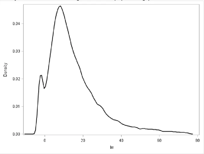
Figure 6
Density functions of returns to higher education (in percentage)
Source: authors’ calculations.
Note: Irr stands for internal rate of return; Irr values above 75% are excluded from the computation of
the density function.
Figure 6 shows that there is a great dispersion of internal rates of return to higher education. This is noteworthy that the risk of having relatively low returns is not symmetric to the risk of having high returns. The lower returns are closer to the modal value than the higher returns. Moreover, there is a decrease in density across the zero value. As shown in Figure 7, this effect corresponds to gender differences in employment patterns across the life cycle—see Appendix figure A3. In this view, the probability of being in a position out of employment and the impact it has on the remaining career—which are captured by our modelling— explain this concentration
27
of values under zero for women. Because of this specific gender effect, we focus our comment of density functions by diploma on men6.
Figure 7
Density functions of returns to higher education (in percentage) by gender
Source: authors’ calculations.
Note: Irr stands for internal rate of return; Irr values above 75% are excluded from the computation of
the density function.
Figure 8, shows that the asymmetric shape is observed for the different diploma classes we pointed out previously—see Table 5. However, the shapes tend to be more symmetric for the highest levels of diploma: namely, the five-year university degrees (U5, box 6), the other five-year degrees (S5, box 7) and the PhD (Up, box 8). This indicates that this latest kind of education produces a more predictable output, and should be preferred by individual who are risk-adverse independently of the
6
The density functions by diploma for women exhibit the same kind of shape than those for men, except that most of these functions exhibit this decrease in density at the zero value.
28
mean level of returns. More generally, these results illustrate how taking into account the valuation risk of diploma may explain education choices for risk-adverse persons.
Figure 8
Density functions of returns to higher education (in percentage) by diploma’s type for men
Source: authors’ calculations.
Note: 1-U2 : DEUG (university two-year degrees); 2-S2: other two-year degrees; 3-U3: licence (university three-year degrees); 4-S3: other three-year degrees; 5-U4 maîtrise (university four-year degrees); 6-U5: university five-year degrees; 7-S5: other five-year degrees; 8-Up: PhD.
Irr stands for internal rate of return; Irr values above 75% are excluded from the computation of the density function.
5. Conclusion
On the basis of a dynamic microsimulation model of the educational outputs for a given generation, we compute a distribution of the returns to tertiary education for France. In this context, our modelling produces indicators which complement the standard OECD indicator of mean return to tertiary education. The main complementary result consists of measuring the risk of low return in pursuing a tertiary education. Producing such indicators at a country level could help to design and monitor cost-sharing policies which are recommended at the European Union level for the development of tertiary education.
29
More precisely, the OECD indicator emphasizes that because of the gap between the mean rate of return to tertiary education and the interest rate, which is v