Use of Discriminant Analysis in Time Series Model Selection

Agada Joseph Oche and Ugwuowo, Fidelis Ifeanyi

Received 12 November2018/Accepted 16 December 2018/Published online: 24 December 2018 Abstract A systematic approach to time series model

selection is very important for reduction of the uncertainties associated with highly subjective and inaccurate method currently being used. Information criteria as a measure of goodness of fit have been criticized because of its statistical inefficiency. In this paper, we develop a rule using discriminant analysis for classification of a time series model from a finite list of parsimonious ARMA (p,q) models. A discriminant function is developed for each of the six alternative ARMA(p,q) models using fifty sets of simulated time series data for each model. An algorithm is developed for the evaluation of discriminant scores and model selection. The selection rule is based on the highest discriminant score among the six alternative models. The method was applied to a real life data and thirty sets of simulated data. The real life application resulted in correct model selection while the simulated data gave 93% correct

classification. Key Words: Time series, model selection, ARMA model,

discriminant analysis, simulated data. Agada Joseph Oche

Headquarters, 051 Personnel Management Group, Nigerian Air Force, Ikeja Lagos

Lagos State, Nigeria *Ugwuowo, Fidelis Ifeanyi Department of Statistics, University of Nigeria, Nsukka Enugu State, Nigeria

Email: [email protected]

1.0 Introduction

In time series model development using Box and Jenkins (1970), it has been observed that no precise formulation of the problem is available at different stages. The stage which involves comparison of the autocorrelation functions (ACF) and partial autocorrelation functions (PACF) obtained from the series for which a model is to be fitted with the known theoretical behavior is subject to individual judgment and therefore inexact (Box, Jenkins and Reinsel, 2008). In all the iterative steps usually taken before the final model is selected, this stage seems to be the most challenging and most ambiguous. In practice, the best model is supposed to be selected in order to ensure accurate forecast. Tsay and Tiao (1984, 1985) proposed the use of extended autocorrelation function (EACF) and smallest canonical correlation (SCAN) respectively for

identifying various orders of autoregressive moving average (ARMA (p,q)) model when

p q

,



0

. Their proposal is even more challenging since comparing EACF and canonical correlation of theoretical models with that of the Series at hand is very difficult as the sample EACF has no clear cut off (Cryer and Chan, 2008). The use of Akaike (1969) and various forms of information criteria in final model selection has been criticized as their approach is based on values calculated from residual of already fitted models which is perceived as information loss from fitting that particular order into the series (Akaike, 1974, 1979, 1980; Bhansali, 1993; Hannan and Quinn, 1979; Schwartz, 1978; Anderson, 2008; Anderson, 1975 and Pukkila, Koreisha and Kallinen, 1990). Also, Shibata (1976) has shown that Akaike information criterion (AIC) tend to overestimate the true order of an AR model while the Bayesian information criterion (BIC) under estimate it. Zazli (2002) in a comparative study concluded that the efficiency of various information criteria depends on where it is being used. He advised that various information criteria be combined to avoid problem associated with inefficiency of respective information criterion. Rayalu, Ravisankar and Mythili (2017) suggested a goodness of fit criterion for ARMA (p, q) model and modified the AIC and SBC but could not show an illustrative example for its use. Jamil and Bouchachia (2019) discussed the problem of selecting model parameters in time series forecasting using aggregation. They proposed a new algorithm that relies on the paradigm of prediction with expert advice, where online and offline autoregressive models are regarded as experts.

Discriminant analysis is a multivariate method that classifies a given observation into one of the available k-classes



k



2



. The proposed model selection procedure is based on the discriminant function. In contrast with Box and Jenkins methodology which only compares the features of the ACF and PACF of the series for which a model is to be fitted with the theoretical features, this approach uses the actual values of those features. Furthermore, it selects a model automatically from a finite list of alternative models. Shah (1997) developed an individual selection rule using discriminant analysis and compared its performance to aggregate selection for the quarterly series of the M-Competition data. The results indicated that the individual selection rule based on discriminant scores is more accurate and sometimes significantly so, than any aggregate selection method. In this paper, we develop a rule for selection of the best autoregressive moving average ARMA (p,q) model using

discriminant analysis. This method combines modified discriminant functions obtained using some structural features of simulated series of a list of ARMA (p, q) models. An algorithm which is to be used alongside the discriminant functions for model selection is also developed.

In section 2, we introduce the model selection using discriminant analysis, the six alternative models, the development of the discriminant function and the proposed algorithm. Results and discussion including the application to both simulated data and real life data are presented in section 3. The conclusions are given in section 4 while the references are in section 5.

2.0 Model selection using discriminant analysis The discriminant function development using the features of a series is based on the normality assumption. The two main analyses that are based on this assumption are the linear discriminant analysis (LDA) and the quadratic discriminant analysis (QDA). The Bayesian quadratic discriminant analysis (QDA) was first proposed by Geisser (1964) and Keehn (1965) and their work has attracted series of subsequent work on the Bayesian QDA (Srivastava, Gupta and Frigyik, 2007).

Consider the population X whose group is k, one of the basic assumptions of discriminant analysis is that k is multivariate normal with parameter



_k and covariance matrix



_k. If we let



_k be the prior probability that an arbitrary unit belong to group

k

defined mathematically as



_k



P G k







, then the Bayes classification rule is given by

P G k X





/



x



which is defined as,

1

( )

(

/

)

( )

k k k j j j

f x

P G k X

x

f x















(1)

Equation (1) is derived from the Bayes theorem hence the name Bayes classification rule (Bickel and Levina, 2004). Compute the posterior probability

P G k X

(



/



x

)

for each class

k

given the observation vector

x

_{and the class}

with the highest value is the most likely class for the unit being considered. Knowing the prior probability, the posterior probability can be calculated and used to predict class membership of an arbitrary series.

Consider

P G k X

(



₁

/



x

)

and

P G k X

(



₂

/



x

)

; class

k

₁ is more likely than

k

₂ if,



1

/





2

/



P G k X x



 

P G k X x





Hence,







12



/

1

/

P G k X

x

P G k X

x











(2)

Substituting the assumed multivariate normal distribution and taking log of both sides gives,

 



 



 



 



1 1 1 1 2 2 2 2 ' ₁ 1 2 2 ' ₁ 1 2 2 1 1 exp 2 2 log 0 1 1 exp 2 2 k k k p k k k k p k x x x x



 





 



   _{   }      _{ }      _  _{ }   _{    }   _        (3)

Therefore, for the observation vector

x

, equation (3) reduces to, log ) x ( ) x ( 2 1 | | log 2 1 log ) x ( ) x ( 2 1 | | log 2 1 2 2 2 2 2 1 1 1 1 1 k k 1 k k k k k 1 k k k                           (4) Generalizing equation (4) we obtain the quadratic discriminant function as,

log ) x ( ) x ( 2 1 | | log 2 1 ) x ( QDF k k 1 k k k k          (5) Group

k

is more likely if equation (5) is highest.

Consider the expression in equation (4), let

     2 1 k

k , then

k

1 is more likely if, 0 log ) x ( ) x ( 2 1 log ) x ( ) x ( 2 1 2 2 2 1 1 1 k k 1 k k k 1 k                       (6) Expanding the expression above and re-arranging we find that, log 2 1 x log 2 1 x 2 2 2 2 1 1 1 1 k k 1 k 1 k k k 1 k 1 k                          (7)

Generalizing equation (7) we obtain the linear discriminant function as,

k k 1 k 1 k k log 2 1 x ) x ( LDF      (8) Given an observation vector

x

, group

k

is more likely if equation (8) is highest.

The use of this function is based on the multivariate normal distribution. Note that when both



_k and



_k are assumed to vary with

k

, the quadratic discriminant

function is adopted but when



_kdiffer with

k

and



_k is the same for all

k

, the linear discriminant function is adopted. The classification rules are the same for both functions and states that given an observation vector

x

, the class

k

for which the discriminant function of

x

is highest is the most likely class of the unit on which

x

is calculated.

The estimated parameters of the two discriminant functions considered are



_k,



,



_k and



_k. If they are plugged directly into the Bayes classification rules, we will obtain Fisher’s classification rules (Bickel and Levina, 2004).

2.1 The Alternative Models

The general class of models to be used in the development of the discriminant function is the ARMA (p, q) model with 0 ≤ p, q ≤ 2. However, for simplicity we restrict the study to six models to be included in the list of alternatives from which selection will be made. They are: AR (1), AR (2), MA (1), MA (2), ARMA (1, 1) and ARMA (2, 2). The lower orders of ACF and PACF of all the models are defined as feature variables for use in the development of the discriminant rule. In ARMA modeling the autocorrelation and partial autocorrelation functions are extensively used in identification stage (Shah, 1997 and box and Jenkins, 1970). The Box and Jenkins approach is characterized by tentative determination of the order of the model, fitting of several models and the use of information criteria to select the best model. However, for ARMA (p,q) model, no tentative model can be chosen accurately since the value of p and q cannot be determined with both ACF and PACF tailing off. These models are also classified according to Box and Jenkins as parsimonious models with parameters lying between 0 ≤ p, q ≤ 2. The problem of choosing the most appropriate feature variables is not simple, (Shah 1997), however, eight feature variables were defined and computed for each series.

2.2 Development of the discriminant function

The proposed model selection procedure is based on the assumption that the ACF and PACF which are within-sample structural features of the series are functions of the selected model (Shah, 1997). In line with Box and Jenkins (1976), these features play a significant role in model selection. They are measurable and their values are used to form the vector

x

of dimension

d

. A discriminant rule is estimated that gives the posterior probability for a series belonging to each of the six models, given its feature vector x. The series is assigned to belong to the group for which the probability is greatest. The discriminant rule is constructed from a data set of n series whose model is known a priori as coming from the alternative list. To

develop the discriminant functions, we simulated 150 known theoretical time series patterns (models) each for the six linear stationary models considered. For each simulated theoretical time series, we obtain the vector



1

,...,

8



x



x

x

where

x

₁

,...,

x

₄ are absolute values of ACF of n sets of time series at lag 1 to 4 respectively;

5

,...,

8

x

x

are absolute values of PACF of n sets of time series at lag 2 to 5. The vector

x





x

₁

,...,

x

₈



is an 8 dimensional multivariate random variable used in developing the discriminant function. The absolute values of these structural features were used to avoid loss of information since model selection considers only the magnitude of ACF and PACF but not the sign. Multivariate normality of the eight dimensional feature vector 𝑥 with mean vector varying with the groups is assumed. The quadratic discriminant rule is adopted following the failure of the test for equality of variance-covariance matrix. For each group say k, the variance-covariance matrix



_k and the mean vector



_k for the variables are calculated. The discriminant function which is developed for group k is now given as follow:

6 & 5 , 4 , 3 , 2 , 1 k where log ) x ( ) x ( 2 1 | | log 2 1 ) x ( Q 1 _{k k} k k k k               (9) Where



_kis the prior probability that the individual or item considered belong to group k. This is assumed equal for all groups and as such is 1/6. The quadratic function is a function of the vector 𝑥. These parameters are calculated and substituted in equation (9) for all the groups.

The model selection rule can be used for various sets of time series data. It is a discriminant function based on six simulated parsimonious theoretical models. The developed quadratic discriminant functions is such that any arbitrary time series can be assigned to the appropriate theoretical model using the discriminant score and the selected model fitted into the series. This approach does not have tentative model selection stages which are traditionally seen in time series modeling. The discriminant scores are highly comparable with the conventional information criteria in terms of behavior. However, while the information criterion chooses the model that minimizes the error terms, the discriminant scores choose the model that maximizes the probability. 2.3 The proposed algorithm for model selection

This proposed algorithm shows the step by step implementation of selecting the best model using discriminant analysis. Given a Series whose theoretical model is to be identified, the summary of the proposed model selection algorithm is presented below:

Step 1: select the models to be included in the list of alternatives and set the criterion for model selection. Step 2: simulate n sets of sample time series data from

the list of alternative models.

Step 3: use the absolute values of the feature variables lag 1-4 of ACF and lag 2-5 of PACF that form an 8-dimensional vector 𝑥 to obtain the discriminant function for each model listed.

Step 4: use the time series of interest and obtain the feature variables lag 1-4 of ACF and lag 2-5 of PACF and denote the observation vector 𝑥 𝑎𝑠 𝑥 = (𝑥 , 𝑥 , 𝑥 , 𝑥 , 𝑥 , 𝑥 , 𝑥 , 𝑥 ).

Step 5: input the vector 𝑥 into each of the six

discriminant functions to obtain the discriminant score.

Step 6: select the model with the highest discriminant score and fit the series.

Step 7: perform a diagnostic test on the fitted model and stop iteration if the model is adequate, else, go back to step 6 and consider the model with the next highest discriminant score.

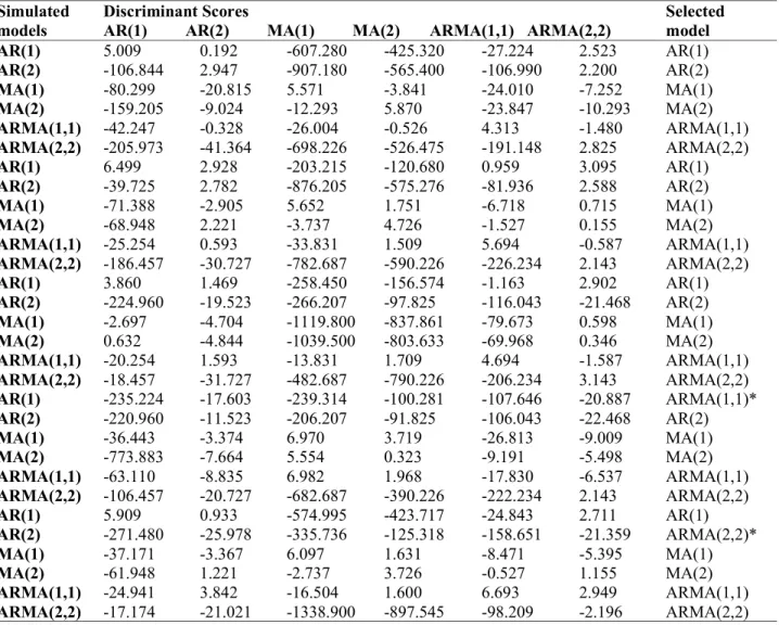
3.0 Results and discussion 3.1 Applications to simulated data

Table 1 shows the discriminant scores obtained using 30 simulated Time Series data. The result shows that twenty eight of the simulated time series were correctly selected after the first iteration while only two were selected in two iterations. This implies that the approach has a 93% correct classification. The algorithm was now used in the selection of the model for each group. This method is limited to ARMA (p,q) models with 𝑝, 𝑞 ≤ 2 _which

represent the orders of the models that are adequate and parsimonious in most cases, (Box and Jenkins, 1970). Table 1: Result of the classification using discriminant scores

.

Simulated models

Discriminant Scores

AR(1) AR(2) MA(1) MA(2) ARMA(1,1) ARMA(2,2)

Selected model AR(1) 5.009 0.192 -607.280 -425.320 -27.224 2.523 AR(1) AR(2) -106.844 2.947 -907.180 -565.400 -106.990 2.200 AR(2) MA(1) -80.299 -20.815 5.571 -3.841 -24.010 -7.252 MA(1) MA(2) -159.205 -9.024 -12.293 5.870 -23.847 -10.293 MA(2) ARMA(1,1) -42.247 -0.328 -26.004 -0.526 4.313 -1.480 ARMA(1,1) ARMA(2,2) -205.973 -41.364 -698.226 -526.475 -191.148 2.825 ARMA(2,2) AR(1) 6.499 2.928 -203.215 -120.680 0.959 3.095 AR(1) AR(2) -39.725 2.782 -876.205 -575.276 -81.936 2.588 AR(2) MA(1) -71.388 -2.905 5.652 1.751 -6.718 0.715 MA(1) MA(2) -68.948 2.221 -3.737 4.726 -1.527 0.155 MA(2) ARMA(1,1) -25.254 0.593 -33.831 1.509 5.694 -0.587 ARMA(1,1) ARMA(2,2) -186.457 -30.727 -782.687 -590.226 -226.234 2.143 ARMA(2,2) AR(1) 3.860 1.469 -258.450 -156.574 -1.163 2.902 AR(1) AR(2) -224.960 -19.523 -266.207 -97.825 -116.043 -21.468 AR(2) MA(1) -2.697 -4.704 -1119.800 -837.861 -79.673 0.598 MA(1) MA(2) 0.632 -4.844 -1039.500 -803.633 -69.968 0.346 MA(2) ARMA(1,1) -20.254 1.593 -13.831 1.709 4.694 -1.587 ARMA(1,1) ARMA(2,2) -18.457 -31.727 -482.687 -790.226 -206.234 3.143 ARMA(2,2) AR(1) -235.224 -17.603 -239.314 -100.281 -107.646 -20.887 ARMA(1,1)* AR(2) -220.960 -11.523 -206.207 -91.825 -106.043 -22.468 AR(2) MA(1) -36.443 -3.374 6.970 3.719 -26.813 -9.009 MA(1) MA(2) -773.883 -7.664 5.554 0.323 -9.191 -5.498 MA(2) ARMA(1,1) -63.110 -8.835 6.982 1.968 -17.830 -6.537 ARMA(1,1) ARMA(2,2) -106.457 -20.727 -682.687 -390.226 -222.234 2.143 ARMA(2,2) AR(1) 5.909 0.933 -574.995 -423.717 -24.843 2.711 AR(1) AR(2) -271.480 -25.978 -335.736 -125.318 -158.651 -21.359 ARMA(2,2)* MA(1) -37.171 -3.367 6.097 1.631 -8.471 -5.395 MA(1) MA(2) -61.948 1.221 -2.737 3.726 -0.527 1.155 MA(2) ARMA(1,1) -24.941 3.842 -16.504 1.600 6.693 2.949 ARMA(1,1) ARMA(2,2) -17.174 -21.021 -1338.900 -897.545 -98.209 -2.196 ARMA(2,2)

3.2. Application to real life data

Consider series A (Chemical Process concentration readings: every two hours) time series data from Box, Jenkins and Reinsel (2008) p. 670 which was modeled as ARMA (1,1). We now apply the model selection algorithm to this series as follows:

Step 1: use the discriminant functions of the six parsimonious alternative models obtained

Step 2: use series A sample data and obtain the absolute values of the ACF at lag 1- 4 and PACF at lag 2-5, to give the vector

x

;

) 07 . 0 , 08 . 0 , 07 . 0 , 24 . 0 , 29 . 0 , 32 . 0 , 42 . 0 , 48 . 0 ( xT _

Step 3: Input the observation vector 𝑥 into each of the discriminant functions to get the resulting discriminant scores as: -87.694, -30.365, -186.053, -117.148, -26.840 and -41.205. for AR(1), AR(2), MA(1), MA(2), ARMA(1,1) and ARMA (2,2) respectively.

Step 4: select ARMA (1, 1) model with the highest score of – 26.840 as the best model

Step 4: stop since the diagnostic check shows that it is adequate.

In conclusion, this real-life application was correctly selected in only a single iteration.

4.0 Conclusions

Model selection is an integral part of the tasks involved in ARMA time series model development. The traditional approach of initially selecting several tentative models and then using information criteria to choose the best is known to have some shortfalls which include but not limited to lack of precise problem formulation and interference of personal judgment. We have adopted an approach which is systematic and different from Box and Jenkins. The approach uses the actual values of ACF from lag 1 - 4 and PACF from lag 2 -5 obtained from the series to be fitted as against the traditional approach that relies on careful examination of the behavior of the sample ACF and PACF.

This approach requires a determination of the discriminant score and using it to select the best model thereby addressing the problems with overlapping nature of identification and estimation stages in the Box and Jenkins approach. The algorithm developed along with the discriminant function is capable of selecting the exact model with very high level of certainty and in event where the selected model is not the appropriate model,

the algorithm also predetermines the next model to be considered.

The correct classification of 93% from the simulated series is quite high and encourages the recommendation of the method. The series A time series data from Box, Jenkins and Reinsel (2008) was correctly selected in only a single iteration. Finally, this method is generally characterized by well-organized rules and procedures for model selection while the Box and Jenkins method is unavoidably characterized by uncertainty due to individual judgment.

Further research is needed in the selection of appropriate set of feature variables. Given a set of eight feature variables used in this work, it is possible that smaller set may significantly discriminate between the sample models.

5.0 References

Akaike, H. (1969). Fitting Autoregressive Models for Prediction. Annals Institute of Statistical Mathematics. 21, pp. 243-247.

Akaike, H. (1974). A new look at the statistical model

identification. IEEE Transactions on Automatic

Control, 19, 6, pp. 716–723.

Akaike, H. (1979). A Bayesian Extension of the Minimum AIC procedure of Autoregressive Model fitting. Biometrika; 66:237-242.

Akaike, H. (1980). Likelihood and the Bayes procedure. in Bernardo, J. M.; et al., Bayesian Statistics, Valencia: University Press, pp. 143–166.

Anderson, D. R. (2008). Model Based Inference in the Life Sciences, Springer.

Anderson, O.D. (1975). Distinguishing between simple Box and Jenkins models. International Journal of Mathematics. Education. In Science. and Technology, 6, 4. Pp. 461-465.

Bhansali, R.J. (1993). Order Selection for Time Series Models: A Review, in development in

Time Series Analysis by Rao, T.S., Chapman and Hall, London.

Bickel, P.J. & Levina, E. (2004). Some theory for Fisher’s Linear Discriminant Function “Naïve Bayes” and some alternatives when there are many more variables than observations. Bernoulli,10, 6, pp. 989-1010.

Box, G.E.P. & Jenkins, G.M. (1970). Time Series Analysis, Forecasting and Control. San Francisco: Holden-Day.

Box, G.E.P & Jenkins, G.M. (1976). Time Series Analysis, Forecasting and Control. San Francisco: Holden-Day. Box, G.E.P., Jenkins, G.M. & Riensel, G.C. (2008). Time Series Analysis: forecasting and control. New Jersey: Wiley.

Cryer, J. D. & Chan, K. S. (2008). TimeSeries Analysis with application in R. Springer. Scienc+Business Media, LLC, 2nd _edition.

Geisser, S. (1964). Posterior odds for multivariate Normal Distribution. Journal of the Royal Statistical Society Series B Methodological, 26, pp.69-76.

Hannan, E. J. & Quinn, B. G. (1979). The Determination of the order of an Autoregressive. Journal of the Royal Statistical Society, Serie, B, 41, pp.190-195.

Jamil W. & Bouchachia A. (2019). Model Selection in Online Learning for Times Series Forecasting. In: Lotfi A., Bouchachia H., Gegov A., Langensiepen C., McGinnity M. (eds) Advances in Computational Intelligence Systems. UKCI 2018. Advances in Intelligent Systems and Computing, vol. 840. Springer, Cham.

Keehn, D. G. (1965). A Note on Learning for Gaussian Properties. IEEE Trans. On Information Theory, 11, pp.126-132.

Pukkila, T., Koreisha, S. & Kallinen, A. (1990). The Identification of ARIMA Models. Biometrika. 77, pp.537-548.

Rayalu, G.M., Ravisankar, J. & Mythili, G.Y. (2017). Goodness of fit and model selection criteria for time series models. IOP Conf. Series: Materials Science and Engineering, 263, 042135 doi:10.1088/1757-899X/263/4/042135

Schwartz, G. (1978). Estimating the Dimension of a Model. Annals of Statistics, 6, pp.461-464.

Shah, C. (1997). Model selection in univariate time series forecasting using discriminant analysis.

International Journal of Forecasting, 13, 4, pp. 489-500.

Shibata, R. (1976). Selection of the order of an Autoregressive Model by Akaike’s Information Criterion. Biometrika, 63, pp. 117-126.

Srivastava, S., Gupta, M.R. & Frigyik, B.A. (2007). Bayesian Quadratic Discriminant Analysis. Journal of Machine Learning Research, 8, pp.1277-1305. Tsay, R. S. & Tiao, G. (1984). Consistent estimates of

autoregressive parameters and extended sample autocorrelation function for stationary and non-stationary ARMA Models. Journal of the American Statistical Association, 79, 385, pp.84–96.

Tsay, R. & Tiao, G. (1985). Use of canonical analysis in time series model identification. Biometrika. 72, pp. 299–315.

Zazli, C. (2002). Performance of order Selection Criterion for Short Time Series. Pakistan