1 INTRODUCTION
Wildfires are a natural hazard with potentially severe economic, social and ecologic consequences. This motivates investigations into the factors influencing wildfire behavior and their utilization for prediction purposes. In this paper, we summarize the development of a Bayesian network (BN) model for predicting wildfire behavior.
Many authors have described the development of probabilistic prediction of wildfire occurrence and behavior using regression models; e.g. in (Brillinger et al., 2003), a generalized additive model is proposed for fitting wildfire occurrence data. BN models for predicting the number of wildfire occurrences were proposed by (Dlamini, 2010, Papakosta and Straub, 2011). In these two papers, the conditional probability tables (CPTs) of the BN are learned from data, while the structure of the BN is introduced by the authors based on process understanding.
Learning of the BN structure as well as its parameters has been previously applied in the fields of natural hazards and environmental modeling. For example, (Kuehn et al., 2011) develop a BN to model the joint probability distribution of earthquake parameters Similarly (Mesbah et al., 2009) develop a BN for modeling water quality in a river. (Alameddine et al., 2011) investigate different constraint-based structure-learning algorithms to establish a BN that predicts chlorophyll levels. They
also consider the sensitivity of these algorithms to the scheme for discretizing random variables. A comparison between BNs with automatically learned structure to a BN constructed from expert knowledge is carried out by (Ordóñez Galán et al., 2009) for an application in reforestation planning.
Our focus is on the prediction of wildfire spreading using BNs. For prediction purposes, a number of observable variables (indicators) are available, which are indirectly related to wildfire spreading. Among the available indicators it is not obvious, which of them are most informative for describing the conditions for wildfire spreading, and which are not informative or redundant. In this paper, structure-learning algorithms are applied to identify the relevant indicators. A final BN model is then developed combining the identified indicators with understanding of the process, and is compared to a Naïve Bayesian Classifier (NBC) model.
The approach is applied to a study area on Cyprus, for which data from 611 wildfires were available.
2 METHODOLOGY 2.1 Bayesian networks
Only a brief summary of Bayesian networks (BNs) is provided. For further information, the reader is referred to introductory textbooks such as (Jensen and Nielsen, 2007).
Learning a Bayesian network model for predicting wildfire behavior
K. Zwirglmaier, P. Papakosta, D. Straub
Engineering Risk Analysis Group, Technische Universität München, Germany
ABSTRACT: A Bayesian network (BN) model for predicting wildfire spreading was developed. From the available indicator variables related to weather, topography and land cover, the most informative were selected with the help of automatic structure learning algorithms. A final BN model was then constructed from these indicators using phenomenological reasoning. Automatic structure learning of the complete model was found to have severe limitations due to large number of variables in combination with limited number of observations. The BN model was learned and validated with data from the Mediterranean island of Cyprus. The final BN was compared to a Naïve Bayesian Classifier (NBC), which serves as a benchmark, and it was shown to be applicable for prediction purposes.
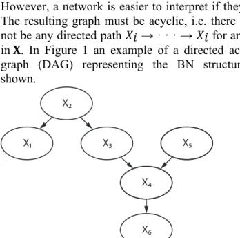
A BN is a graphical representation of a joint probability distribution 𝐹𝐹(𝐗𝐗) of a set of random variables 𝐗𝐗. Each variable 𝑋𝑋𝑖𝑖 in 𝐗𝐗 is represented by a node. The nodes in a BN are connected by directed links, which represent the statistical dependence structure among variables. The directions of the links do not necessarily have to represent causality. However, a network is easier to interpret if they do. The resulting graph must be acyclic, i.e. there must not be any directed path 𝑋𝑋𝑖𝑖 → · · · → 𝑋𝑋𝑖𝑖 for any 𝑋𝑋𝑖𝑖 in 𝐗𝐗. In Figure 1 an example of a directed acyclic graph (DAG) representing the BN structure is shown.
Figure 1 Example of a directed acyclic graph (DAG) representing the BN structure.
To each of the nodes 𝑋𝑋𝑖𝑖 a conditional probability table (CPT) is attached. This CPT is the distribution of the random variable 𝑋𝑋𝑖𝑖, conditional on its parents. The CPTs of all 𝑋𝑋!s together with the DAG completely define the joint probability distribution of 𝐗𝐗.
The DAG of a BN reveals which variables are statistically dependent for given evidence. If e.g. two variables are dependent, additional evidence that is obtained for one of them will alter the distribution of the other variable. Variables that are dependent are said to be d-connected; if they are independent they are said to be separated (Pearl, 1988). The d-separation properties of the BN are directly related to the Markov blanket of a node. The Markov blanket of a variable 𝐴𝐴 consists of the parents and the children of 𝐴𝐴 and all other parents of 𝐴𝐴′𝑠𝑠
children. If all the variables in the Markov blanket of a node 𝐴𝐴 are known, 𝐴𝐴 is d-separated (and thus independent) of all remaining variables in the BN.
2.2 Structure learning
A DAG for a BN is often constructed from expert knowledge. If one knows how the variables influence each other, a graph representing these causal relations can be developed. For applications
where such knowledge is unavailable, observations can be used to automatically learn the structure. Two different approaches for learning a BN structure exist:
• In the score-based approach, a number of
candidate graphs are generated and the one that is best according to some score (like the Bayesian information criterion BIC or the Akaike information criterion AIC) is chosen.
• The constraint-based approach derives a set
of conditional and unconditional independence properties from the data. Then a DAG is constructed, which represents these independence properties as accurately as possible.
In this paper, constraint-based algorithms are used to learn parts of the BN, in order to identify relevant indicators. The structure of the eventual BN model is constructed from understanding of the process. Finally a score-based approach is applied to compare this BN to a reference NBC model.
In the following, two of the most important constraint-based algorithms, the PC algorithm (Spirtes et al., 2001) and the NPC algorithm (Steck and Tresp, 1999, Steck, 2001) are explained and compared by an example.
Both constraint-based algorithms take two steps in order to come up with a DAG for a BN. In a first step, an undirected graph is derived. The links of this undirected graph coincide with those of the eventual DAG, however they are not oriented. In a second step, these links are oriented.
Both algorithms perform independence tests on a dataset, i.e. for each pair of variables they search for a set of nodes, such that these two variables are conditionally (on this set of nodes) independent according to the data. For example, 𝐼𝐼(𝐴𝐴, 𝐵𝐵|𝐒𝐒) means that the variables 𝐴𝐴 and 𝐵𝐵 are found to be conditionally independent if all variables in 𝐒𝐒 are known. They are not independent if only a subset of
𝐒𝐒 is known. If two variables are unconditionally independent, S is the empty set. For further information on independence tests we refer to (Spirtes et al., 2001). The aim of both the PC and the NPC algorithm is now to find a DAG, which represents the independence properties of an underlying distribution as suggested by the data.
For illustration purposes, we consider the following example with four variables 𝐴𝐴, 𝐵𝐵, 𝐶𝐶 and
𝐷𝐷. From the available data, it is found that A and D are independent, i.e. 𝐼𝐼(𝐴𝐴, 𝐷𝐷). Furthermore, the following conditional independence properties were identified: 𝐼𝐼(𝐴𝐴, 𝐵𝐵|𝐶𝐶), 𝐼𝐼(𝐵𝐵, 𝐶𝐶|𝐴𝐴) and 𝐼𝐼(𝐵𝐵, 𝐷𝐷|𝐶𝐶). For all the other pairs of nodes, no sets of nodes are X1 X2 X3 X4 X5 X6
found, such that they are conditionally independent. Note that the tests are performed so that the conditioning set 𝐒𝐒 is minimal, i.e. the pairs with identified independence properties are not independent given any real subset of 𝐒𝐒. As an example, 𝐴𝐴 and 𝐵𝐵 are not independent if 𝐶𝐶 is not known.
When two variables are found to be conditionally or unconditionally independent, it is desired that their corresponding nodes are d-separated respectably in the DAG. For two nodes to be d-separated in a graph, they must not be connected through a direct link. For this reason, the PC algorithm ensures that no links exist between any pairs of variables that were found to be independent, either conditionally or unconditionally. Starting from a complete undirected graph, all links between variables with identified independence properties are deleted. In our example, the links [𝐴𝐴, 𝐷𝐷], [𝐴𝐴, 𝐵𝐵],
[𝐵𝐵, 𝐶𝐶] and [𝐵𝐵, 𝐷𝐷] are deleted and the resulting undirected graph is as shown in Figure 2. According to this solution, B would be d-separated from all other nodes under all circumstances, implying that B is unconditionally independent of all other variables. Clearly, this is in contradiction to the identified independence properties, which state that 𝐵𝐵 is only conditionally independent of 𝐴𝐴, 𝐶𝐶 and 𝐷𝐷.
Figure 2 Undirected graph obtained from the PC algorithm.
The PC algorithm will lead to the correct, undirected graph, if the distribution can be represented in a DAG and if all the derived independence properties are actual properties of the underlying distribution and not due to some random noise (Steck, 2001). However, in many applications, where only a limited number of observations are available, the identified independence properties are influenced by random noise. In the considered example, the PC algorithm leads to inconsistencies, as discussed above. It is not possible to say whether this is because of random noise or because the true distribution cannot be represented by a graphical model.
The NPC (necessary path condition) algorithm tries to overcome the problem of random noise by checking the derived independence properties for
consistency. Roughly speaking, the necessary path condition states, that a node 𝐶𝐶 can only cause two nodes 𝐴𝐴 and 𝐵𝐵 to be d-separated, if there is a path from 𝐴𝐴 to 𝐶𝐶 not crossing 𝐵𝐵 and a path from 𝐵𝐵 to 𝐶𝐶
not crossing 𝐴𝐴.
Instead of directly removing the links between pairs of nodes that were found to be independent, the NPC establishes a condition for each of those links. These conditions state that in order to remove a link between two conditionally independent nodes, there must be a link between each of them, and all the nodes that they were found to be conditionally independent on. This corresponds to the shortest possible necessary path.
For our example, these conditions are condition I to IV in Table 1. Exemplarily, condition II states that the link [𝐴𝐴, 𝐵𝐵] can be removed if there are links between 𝐴𝐴 and 𝐶𝐶 as well as between 𝐵𝐵 and 𝐶𝐶.
Looking at Table 1, we find that there are links that appear in the third as well as in the fourth column. On the one hand, these links are to be removed, as they link two nodes that were found to be independent; on the other hand, these links are needed to fulfill a necessary path condition. If this is the case for a pair of links, the NPC algorithm tries to come up with a new necessary path. For example, condition IV states that the link [𝐵𝐵, 𝐷𝐷] can be removed as long as the links [𝐵𝐵, 𝐶𝐶] and [𝐷𝐷, 𝐶𝐶] exist. However, the link [𝐵𝐵, 𝐶𝐶] is to be removed according to condition III. In this case, condition IV can be reformulated to condition IV’ by inserting III into it. If now either condition IV or condition IV’ can be fulfilled in a graph, the link [𝐵𝐵, 𝐷𝐷] can be removed. For condition II and III it is not possible to identify a new necessary path, because the link [𝐵𝐵, 𝐶𝐶] is required by condition II and [𝐴𝐴, 𝐵𝐵] is required by condition III. For this reason, either the property
𝐼𝐼(𝐴𝐴, 𝐵𝐵|𝐶𝐶) or 𝐼𝐼(𝐵𝐵, 𝐶𝐶|𝐴𝐴) can not be represented in the final DAG. Therefore, [𝐴𝐴, 𝐵𝐵] and [𝐵𝐵, 𝐶𝐶] are referred to as inconsistent links.
Table 1 Conditions for removing links between independent variables, which were established by the NPC algorithm.
Conditio
n Property If (remove) Then (keep)
I 𝐼𝐼(𝐴𝐴, 𝐷𝐷) [𝐴𝐴, 𝐷𝐷] -
II 𝐼𝐼(𝐴𝐴, 𝐵𝐵|𝐶𝐶) [𝐴𝐴, 𝐵𝐵] 𝐴𝐴, 𝐶𝐶 , [𝐵𝐵, 𝐶𝐶]
III 𝐼𝐼(𝐵𝐵, 𝐶𝐶|𝐴𝐴) [𝐵𝐵, 𝐶𝐶] 𝐵𝐵, 𝐴𝐴 , [𝐶𝐶, 𝐴𝐴]
IV 𝐼𝐼(𝐵𝐵, 𝐷𝐷|𝐶𝐶) [𝐵𝐵, 𝐷𝐷] 𝐵𝐵, 𝐶𝐶 , [𝐷𝐷, 𝐶𝐶]
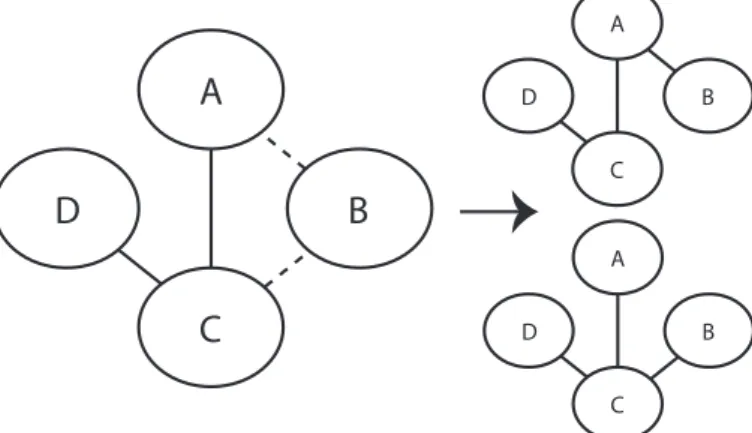
IV’ 𝐼𝐼(𝐵𝐵, 𝐷𝐷|𝐶𝐶) [𝐵𝐵, 𝐷𝐷] 𝐵𝐵, 𝐴𝐴 , [𝐶𝐶, 𝐴𝐴], [𝐷𝐷, 𝐶𝐶] In the left graph of Figure 3, the inconsistent links are shown with dashed lines. The links, which do not correspond to inconsistencies, coincide with the links of the graph found by the PC algorithm in
D B
C A
Figure 2. However, in order to only violate a minimal number of the identified properties, one of the inconsistent links also needs to be present. On the right-hand side of Figure 3, the two possible graphs are presented.
The approaches used to orient the links in the undirected graph are different for the two algorithms. However, in both cases converging connections are oriented first, as it was shown in (Verma and Pearl, 1991) that two DAGs are equivalent, if they have identical links (independent of direction) and the link directions in all converging connections coincide. After that the remaining edges are oriented in a way that no further converging connections and no directed cyclic paths are created.
Figure 3 Undirected graphs learned from the same data as the graph in Figure 2, but with the NPC algorithm. The links [A,B] and [B,C] are not consistent (left), therefore there are two possible solutions (right).
In many real world applications, the number of variables to consider is large, but there are only a limited number of observations from which the structure can be learned. In these cases, structure learning becomes difficult because of the inconsistencies. However, even if it is not desired to learn the complete structure from data, we suggest that structural learning algorithms can still be useful when it comes to identifying relevant indicator variables.
For the sake of illustration, assume that the variable 𝐷𝐷 is the target variable in the structure of Figure 3 learned with the NPC algorithm. We therefore are interested in identifying indicators that influence 𝐷𝐷, which are the variables in 𝐷𝐷’𝑠𝑠 Markov blanket. Regardless of the direction of the link
[𝐷𝐷, 𝐶𝐶], 𝐶𝐶 is part of 𝐷𝐷’s Markov blanket.
Furthermore, A is part of it, if the links [𝐷𝐷, 𝐶𝐶] and
[𝐴𝐴, 𝐶𝐶] are oriented such that 𝐶𝐶 is a common child
of 𝐷𝐷 and 𝐴𝐴. In order to find out if 𝐵𝐵 is relevant, we have to consider multiple possible versions of the graph. If 𝐵𝐵 is in none of the possible directed graphs in the Markov blanket of 𝐷𝐷, we can consider it to be
not relevant. In the current example, we would consider 𝐵𝐵 to be relevant only if 𝐶𝐶 was a common child of 𝐵𝐵 and 𝐷𝐷.
2.3 Discretization of continuous random variables In BNs, usually discrete random variables are used, as the possibilities to perform inference with continuous random variables in BNs are still limited. Observations from the real world are often continuous in their nature. Therefore, continuous random variables need to be discretized in advance. A good discretization should ensure that as little information as possible is lost while having a reasonably small number of intervals (Kotsiantis and Kanellopoulos, 2006).
A number of algorithms for discretizing continuous variables exist. For a review on different discretization techniques, the reader is referred to (Kotsiantis and Kanellopoulos, 2006). In many approaches, the indicator variables are discretized in a way that their interdependence to an already discretized target variable (i.e. the variable, which is to be predicted) is maximized according to some measure of interdependence. In this paper, we apply the class-attribute interdependence maximization (CAIM) measure (Kurgan and Cios, 2004). These approaches are however only capable of maximizing the interdependency between an indicator variable and the target variable. They do not consider that some indicator variables may develop a significant interdependency to the target variable only if they are considered together. Techniques, which do consider this also, are referred to as “dynamic discretization” (Kotsiantis and Kanellopoulos, 2006).
3 LEARNING A WILDFIRE BEHAVIOR PREDICTION MODEL
As a case study, a BN to predict fire behavior in the Republic of Cyprus is learned. Cyprus is located in the Mediterranean region, which is prone to wildfires, mainly due to its climate that is characterized by long, hot and dry summers and mild, wet winters (Pyne, 2009). Further details on the case study area are provided in (Papakosta and Straub, 2013).
In the scope of this work the term wildfire refers to all types of wild-land fires. Furthermore wildfire behavior is described through the burnt area. Other characteristics, such as spread rate, energy release or fuel consumption, are not included here. The main factors governing wildfire behavior are the types and amount of organic fuels and their moisture as well as
D B C A D B C A D B C A
wind and topography (Dupuy, 2009). A BN for predicting wildfire behavior should therefore contain indicators, which accurately describe these main influencing factors. In the current case study, the most important, available data for this purpose is:
Fire Data: Between 2006 and 2010, 611 wildfire occurrences were recorded in the study area. This fire data includes information on date location and the size of the burnt area.
Weather data: Daily noon values of dry-bulb temperature, relative humidity, wind speed, wind direction, as well as accumulated precipitation of the last 24 hours are observed at five weather stations (Papakosta and Straub, 2013).
Fire behavior indices: As part of the Canadian Fire Weather Index System (CFWIS) (Lawson and Armitage, 2008), a number of indices are calculated, mainly from weather data, in order to rate fire risk. The fine fuel moisture code index (FFMC), the initial spread index (ISI) and the buildup index (BUI) are used here. The FFMC describes the moisture content of the litter and cured fine fuels. The ISI is intended to describe the initial rate of fire spreading. In its calculation, the FFMC and the wind speed are used. The BUI represents the amount of material available for combustion as fuel.
Land cover: Descriptions of the land use type with three different levels of detailing are available. They follow the methodology of the Coordination of information on the environment (CORINE) Land cover program (Perdigão et al., 1997).
Topographic data: From a Digital Elevation Model (DEM), slope and aspect are derived for each location, using GIS software.
Based on the above listed available indicators, the relevant factors for fire behavior are to be described, i.e. amount, type and moisture of fuels as well as topography and wind.
Wind and topography are characterized by the directly observable variables wind speed, wind direction, slope and aspect. The relative direction of the wind to the slope, which is an important parameter for fire spreading, is included as the difference between aspect and wind direction.
Type and amount of fuel are considered to be described by the indicator land cover. With the available indicators, the influencing factor most difficult to represent may be fuel moisture. Although fuel moisture is a major part of the indices from the CFWIS, it was found in (Papakosta and Straub, 2011) that the fine fuel moisture code, FFMC, may not suit the Mediterranean climate well for predicting wildfire occurrence, and it may thus also not be ideal for predicting wildfire behavior. Therefore, in addition to the CFWIS indices, direct
weather observations are included in the set of potential indicator variables. These include precipitation, temperature and relative humidity, either on the day of the fire occurrence or mean/cumulative quantities for a number of days prior to the occurrence.
In order to select the variables that are most informative and not redundant, a structure with cumulative/mean variables (for 1, 3, 7, 14 and 21 days before the fire occurrence) together with the variables for the quantities on the day of the occurrence, the CFWIS indices and the target variable, is learned. As mentioned in section 2.2, structure learning has limitations when many variables are present. To limit the number of variables, DAG structures are learned separately for variables describing temperature, relative humidity and precipitation, respectively.
As an example, Figure 4 shows a structure consisting of potential indicator variables related to precipitation. Even in this smaller structure, the NPC algorithm finds inconsistent links, which are shown as dashed lines. To further reduce inconsistencies, the black directed links were introduced as prior constraints. In the graph of Figure 4 there are two different types of inconsistent links (shown with different line styles). Inconsistent links of the same type influence each other. As an example, the presence or the orientation of the link [Burnt Area, Cum. Prec. 21d] will influence either the presence or the orientation of the link [Burnt Area, BUI]. It will not influence the other inconsistent links, as they belong to a different group (shown in a different line style). These groups are known as ambiguous regions in the literature (Steck, 2001).
Depending on the orientation of the uncertain links attached to the target variable, the Markov blanket of the target variable can consist of either the FFMC, the BUI and the cumulative precipitation of the previous 21 days, or of these three nodes together with the parents of the latter two. Using BN software one can resolve the structure, such that one obtains the different possible versions of the DAG. For the graph in Figure 4, both inconsistent links attached to the target variable, were found to be oriented towards it in every version of the DAG. Therefore, it is concluded that the connection is converging and that the FFMC, the BUI and the cumulative precipitation from the previous 21 days were taken to be informative for predicting the burnt area.
For the final BN model, the indicators that were chosen to be relevant (either through understanding of the process or through the structure learning method discussed above), are divided into groups of nodes, which are assumed to significantly influence
each other. Dependencies within these groups are modeled through hidden variables. The hidden variables are not observed, however their parameters can be learned using the expectation-maximization (EM) algorithm (Dempster et al., 1977). The main advantage of hidden variables is that they can represent the joint influence of a set of variables and thus reduce the number of links to the target variable (Straub and Der Kiureghian, 2010). In this way, the number of parameters needed to specify the model can often be significantly reduced.
Figure 4 Result obtained from learning the structure of a set of indicator variables related to precipitation with the NPC algorithm. The black arrows represent prior constraints. The grey links are the directed links that could be learned without ambiguity. The undirected dashed links represent links, for which a consistency problem was found. Note that the inconsistent links with the same line style influence each other.
3.1 The final model
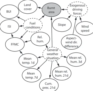
The indicator variables, which are considered to be relevant, are included in the final BN model shown in Figure 5. For example, the three variables ‘BUI’, ‘FFMC’ and Mean ‘Cum. prec. 21d’ were found to be relevant from the learned structure in Figure 4 and are therefore included in the final model.
All relevant indicators are divided into groups. A first group contains the nodes ‘Wind speed’, ‘Slope’ and ‘Aspect-wind-direction-difference’. Different combinations of these driving forces are represented in the unobservable and therefore hidden variable ‘Exogenous driving forces’.
In order to model dependencies between the nodes ‘BUI’, ‘ISI’ and ‘FFMC’, the hidden variable ‘Fuel conditions’ is introduced as a common parent.
Similarly, the hidden variable ‘General weather situation’ is introduced as parent to the variables containing weather information. The ‘FFMC’ and the ‘Temperature of the previous day’ as well as the ‘FFMC’ and the ‘ISI’ are assumed to be directly connected, because of the way the CFWIS indices are calculated.
The variable ‘Land cover’ has 13 distinct states. In order to reduce the number of parameters needed to specify the CPT of the target variable, ‘Land cover’ is modeled as its child. This is contrary to causality, as one would assume that land cover type influences the burnt area and not vice-versa. This has some non-intuitive consequences: In the case, where only the land cover type is observed and all other nodes are unknown, the observation of the ‘Land cover type’ will influence the probability of all other indicators, i.e. they are d-connected. However, this is not critical in most applications because usually all indicators are observed and their dependence structure is thus irrelevant.
All continuous nodes with the exception of ‘Wind speed’, ‘Aspect-wind-direction-difference’ and ‘Slope’ where discretized using the CAIM algorithm (c.f. section 2.3). These three variables are likely to have a significant influence on the target variable only if they are considered in combination. Since the CAIM algorithm does not capture such interdependencies between attribute variables, these three variables are discretized using equal frequency discretization (Dougherty et al., 1995).
Figure 5 A BN model for predicting wildfire spreading. The target node is displayed in grey and the hidden variables with dashed boundaries.
FFMC Cum. Prec. 21 d BUI Burnt Area Cum. Prec. 14 d Cum. Prec. 7 d Cum. Prec. 3 d Cum. Prec. 1 d ISI Prec. Burnt area BUI Land cover ISI FFMC Fuel conditions General weather situation Rel. hum. Mean rel. hum. 21d Mean temp. 1d Mean temp. 7d Mean rel. hum. 3d Cum. prec. 21d Exogenous driving forces Wind speed Slope Aspect-wind dir. difference
3.2 Results
In order to validate the model, the set of available cases is divided into two parts, where one part is used to learn the model and the other one to test the accuracy of the predictions. The data from fires occurring in 2009 were used for validation, since 2009 was the year with the smallest number of fire occurrences (89).
As a benchmark, a Naïve Bayesian Classifier (NBC) model is used. This reference model is composed of the same variables as the BN in Figure 5. However, in the DAG of the NBC model, all indicator variables have the target variable as their only parent. The advantage of this type of model is that inference is easy and the CPTs are kept small. The disadvantage of the NBC is that it is not always capable of representing the true joint distribution of the involved variables, due to its simplicity. NBC models have shown to perform well when it comes to classification tasks, i.e. where only the most likely state of the target variable is of interest (Jensen and Nielsen, 2007).
At first, the mode of the predicted distribution is compared to the actual observed burnt area. This comparison is carried out through a so-called confusion matrix, which is shown in Table 2. For each combination of predicted interval and observed interval, it presents the number of corresponding cases. Here, the frequencies of the reference NBC are shown in brackets.
The confusion matrix seems to indicate that both models have similar classification performance. A single measure for such classification performance is Cohen’s κ-index (Cohen, 1960). This index is 0 if the classifications by the model are as good as a “classification by chance”. The κ-index is 1 if all cases used for validation were classified correctly. For the current case (i.e. predicting the cases from 2009 with models learned from the remaining years’ data), the κ-index for the final BN is 0.35 and 0.36 for the reference NBC.
The κ-index, as well as the confusion matrix, accounts only for the mode of the predicted distribution. In many cases, the entire distribution is of interest, in particular when risk is to be calculated. The entire distribution is considered when comparing the likelihood (or its logarithm) of a test dataset. The log-likelihood is calculated as:
𝐿𝐿𝐿𝐿 𝐝𝐝|𝑀𝑀 = log!" Pr 𝑑𝑑!|𝑀𝑀 ! !!! = log!" Pr 𝑑𝑑! 𝑀𝑀 ! !!! (1)
where 𝐝𝐝 is the validation dataset with 𝑛𝑛 = 89 cases and 𝑑𝑑! is the i-th case in 𝐝𝐝. 𝑀𝑀 is the model. The likelihood of the BN in Figure 5 is -37.6; the log-likelihood of the reference NBC is -40. Therefore, the observations made in 2009 are about 250
≈ 10!!".! 10!!" times more likely according to the final BN model.
Table 2 A confusion matrix comparing the intervals of the burnt area [ha] predicted by the BN vs. the actually observed intervals. The number of cases obtained with the reference NBC are shown in brackets.
True interval Pr ed ict ed in te rv al [0,1] (1,10] (10,100] (100, ∞) [0,1] 42(39) 10(9) 4(4) 0(0) (1,10] 4(7) 13(14) 10(8) 1(2) (10,100] 2(1) 1(0) 0(3) 0(0) (100, ∞) 0(1) 0(1) 1(0) 1(0) 4 DISCUSSION
It has been shown that probabilistic predictions of wildfire spreading are possible with a BN, which uses only easily observable data about land cover, weather and topography. This prediction is more accurate for small fires, which occur more frequently and which therefore are better represented in the data set available for learning the parameters of the model. With more observations predictions may get better for medium large and large fires as well.
The burnt area is likely to be influenced by human factors, in particular the response time, i.e. how fast a fire is recognized and extinguished. Predictions may therefore be improved if these factors are also considered. Alternatively, one could predict the spreading rate of a fire rather than the burnt area directly. However, it is more difficult to collect historic data describing the spreading characteristics of past fire events.
The continuous indicator variables (with the exception of wind, slope and their respective directions) were discretized separately with respect to the target variable. This approach does not consider interdependencies between the indicators. A more optimal discretization scheme for the specific problem could probably be found if dynamic discretization would be applied, which can consider such interdependencies.
5 CONCLUSION
A Bayesian network (BN) model to predict the burnt area due to a wildfire was developed.
Constraint-based BN learning algorithms were applied to identify relevant indicators for the prediction. A final BN was constructed based on these indicators and understanding of the process. The final BN model is validated and shown to be applicable for prediction purposes.
REFERENCES
ALAMEDDINE, I., CHA, Y. & RECKHOW, K. H. (2011) An evaluation of automated structure learning with Bayesian networks: An application to estuarine chlorophyll dynamics. Environ. Model. Softw., 26, 163-172.
BRILLINGER, D. R., PREISLER, H. K. & BENOIT, J. W. (2003) Risk Assessment: A Forest Fire Example. Lecture Notes-Monograph Series, 40, 177-196.
COHEN, J. (1960) A Coefficient of Agreement for Nominal Scales. Educ. Psychol. Meas., 20,
37-46.
DEMPSTER, A. P., LAIRD, N. M. & RUBIN, D. B. (1977) Maximum Likelihood from Incomplete Data via the EM Algorithm. J. Roy. Stat. Soc. B Met., 39, 1-38.
DLAMINI, W. M. (2010) A Bayesian belief network analysis of factors influencing wildfire occurrence in Swaziland. Environ. Model. Softw., 25, 199-208.
DOUGHERTY, J., KOHAVI, R. & MEHRAN, S. (1995) Supervised and Unsupervised Discretization of Continuous Features. Proc. 12th ICML. San Francisco.
DUPUY, J.-L. (2009) Fire Start and Spread. IN BIROT, Y. (Ed.) Living with Wildfires: What Science Can Tell Us. Joensuu, Finland, European forest institute.
JENSEN, F. V. & NIELSEN, T. D. (2007) Bayesian networks and decision graphs, New York [u.a.], Springer.
KOTSIANTIS, S. & KANELLOPOULOS, D. (2006) Discretization techniques: A recent survey. GESTS International Transactions on Computer Science and Engineering, 32,
47-58.
KUEHN, N. M., RIGGELSEN, C. & SCHERBAUM, F. (2011) Modeling the Joint Probability of Earthquake, Site, and Ground-Motion Parameters Using Bayesian Networks. B. Seismol. Soc. Am., 101, 235-249.
KURGAN, L. A. & CIOS, K. J. (2004) CAIM discretization algorithm. IEEE T. Knowl. Data En., 16, 145-153.
LAWSON, B. D. & ARMITAGE, O. B. (2008) Weather guide for the Canadian Forest Fire Danger Rating System, Edmonton, Alberta, Natural Resources Canada, Canadian Forest Service, Northern Forestry Centre.
MESBAH, S. M., KERACHIAN, R. & NIKOO, M. R. (2009) Developing real time operating rules for trading discharge permits in rivers: Application of Bayesian Networks. Environ. Model. Softw., 24, 238-246.
ORDÓÑEZ GALÁN, C., MATÍAS, J. M., RIVAS, T. & BASTANTE, F. G. (2009) Reforestation planning using Bayesian networks. Environ. Model. Softw., 24, 1285-1292.
PAPAKOSTA, P. & STRAUB, D. (2011) Effect of Weather Conditions, Geography and Human Involvement on Wildfire Ignition: A Bayesian Network Model. Proc. 11th ICASP. Zürich, CRC Press.
PAPAKOSTA, P. & STRAUB, D. (2013) Probabilistic prediction of fire occurrence in the Mediterranean. Submitted to Int. J. Wildland Fire
PEARL, J. (1988) Probabilistic reasoning in intelligent systems: networks of plausible inference, San Francisco, CA, Kaufmann. PERDIGÃO, V., ANNONI, A. & CENTRE, C. O.
T. E. C. J. R. (1997) Technical and Methodological Guide for Updating CORINE Land Cover Data Base, ECSC-EC-EAEC.
PYNE, S. J. (2009) Eternal Flame: An Introduction to the Fire History of the Mediterranean. IN CHUVIECO, E. (Ed.) Earth Observation of Wildland Fires in Mediterranean Ecosystems. London, Springer.
SPIRTES, P., GLYMOUR, C. N. & SCHEINES, R. (2001) Causation, prediction, and search, Cambridge. Mass. [u.a.], MIT Press.
STECK, H. (2001) Constraint based structural learning in Bayesian networks using finite data sets, TU München, PhD Thesis.
STECK, H. & TRESP, V. (1999) Bayesian belief networks for data mining. Proc. 2nd Workshop DMDW99. Magdeburg.
STRAUB, D. & DER KIUREGHIAN, A. (2010) Bayesian Network Enhanced with Structural Reliability Methods: Methodology. J. Eng. Mech., 136, 1248-1258.
VERMA, T. & PEARL, J. (1991) Equivalence and synthesis of causal models. Proc. 6th Annual Conference UAI. Elsevier Science Inc.