Bayesian Regularisation in Structured Additive Regression Models for Survival Data

Susanne Konrath & Thomas Kneib & Ludwig Fahrmeir

Bayesian Regularisation in Structured

Additive Regression Models for Survival Data

Technical Report Number 35, 2008 Department of Statistics

University of Munich

Bayesian Regularization and Smoothing Priors

for Survival Data

Susanne Konrath, Thomas Kneib, Ludwig Fahrmeir Department of Statistics, Ludwig-Maximilians-University Munich

ABSTRACT:

During recent years, penalized likelihood approaches have attracted a lot of interest both in the area of semiparametric regression and for the regularization of high-dimensional regression models. In this paper, we introduce a Bayesian formulation that allows to combine both aspects into a joint regression model with a focus on hazard regression for survival times. While Bayesian penalized splines form the basis for estimating nonparametric and flexible time-varying effects, regularization of high-dimensional covariate vectors is based on scale mixture of normals priors. This class of priors allows to keep a (conditional) Gaussian prior for regression coefficients on the predictor stage of the model but introduces suitable mixture distributions for the Gaussian variance to achieve regularization. This scale mixture property allows to device general and adaptive Markov chain Monte Carlo simulation algorithms for fitting a variety of hazard regression models. In particular, unifying algorithms based on iteratively weighted least squares proposals can be employed both for regularization and penalized semiparametric function estimation. Since sampling based estimates do no longer have the variable selection property well-known for the Lasso in frequentist analyses, we additionally consider spike and slab priors that introduce a further mixing stage that allows to separate between influential and redundant parameters. We demonstrate the different shrinkage properties with three simulation settings and apply the methods to the PBC Liver dataset.

KEY WORDS:

Bayesian Lasso; hazard regression; Laplace prior; penalized splines; regularization priors; scale mixtures of normals.

1

Introduction

In recent years, penalization approaches have emerged as a general tool that allows to address different problems in applied regression analyses. On the one hand, penalization has been considered for regularizing regression models with a large number of covariates, where penalization introduces shrinkage of estimated coefficients towards zero (e.g. Goeman, 2007, Park and Hastie, 2006 or Efron, Hastie, Johnstone and Tibshirani, 2004). The ultimate goal is to separate between important, influential variables and nuisance covariates that are not associated with the response. On the other hand, smoothness penalties have a long tradition in semiparametric regression, with smoothing splines and penalized polynomial splines as the most prominent examples (see Wood, 2006 or Ruppert, Wand and Carroll, 2003 for overviews). In this case, the penalty represents a roughness measure for unknown functions that avoids overly flexible function estimates. In this paper, we introduce a unifying Bayesian perspective and general Markov chain Monte Carlo (MCMC) simulation algorithms that allow to combine both regularization and smoothing into a general framework. This unifying concept is applied to hazard regression models for continuous time survival analyses based on either the full or the partial likelihood but can also be applied to other types of regression models such as exponential family regression.

From a Bayesian perspective, adding a penalty term to the likelihood corresponds to the assignment of an informative prior distribution to the regression coefficients. More specifically, the penalty term coincides with the negative log-prior, leading to the equivalence of penalized likelihood and posterior mode estimates. For example, the Bayesian analogue of the quadratic ridge penalty is an i.i.d. Gaussian prior, whereas an i.i.d. Laplace prior corresponds to the Lasso (Park and Casella, 2008). The squared difference penalty typically applied in penalized spline smoothing (Eilers and Marx, 1996) relates to a Gaussian random walk assumption for the polynomial spline coefficients (Lang and Brezger, 2004, Brezger and Lang, 2006). For Gaussian prior distributions, efficient proposal densities for exponential family and hazard regression can be derived based on iteratively weighted least squares (IWLS) proposals as introduced by Gamerman (1997) in the context of random effects models (see Brezger and Lang, 2006 for exponential family regression and Hennerfeind, Brezger and Fahrmeir, 2006 for hazard regression). Since the density of the Gaussian prior for the regression coefficients is differentiable, the corresponding full conditionals can be approximated with a Taylor series expansion. The general idea of IWLS proposals is then to obtain a Gaussian proposal by matching the mode and the curvature of the full conditional based on the Taylor expansion. This

proposal has two advantages: Firstly, it can be used with multivariate coefficient vectors to take correlations into account in the proposals and, secondly, it automatically adapts to the form of the full conditional thereby avoiding manual tuning of the proposal densities.

Park and Casella (2008) demonstrate how a convenient feature of the Laplace prior allows to construct a Gibbs sampler for Gaussian response models. The Laplace prior can be represented as a scale mixture of normals prior with an exponential mixing hyperprior on the variance. This leads to a hierarchical prior formulation, where Gaussian priors are assigned to the regression coefficients whereas adapted hyperpriors for the variances induce the desired regularization properties. We will employ this representation to extend IWLS proposals in non-Gaussian regression models to spiked regularization priors like the Lasso. Note that the scale mixture of normals class is actually quite large, as demonstrated for example in Griffin and Brown (2005) and other types of regularization priors than the Lasso may be considered in the same framework.

We will employ such extended scale mixtures to address one inherent difficulty with sampling based estimation of regularized regression coefficients: Since estimation is based on samples from the posterior, the posterior mean or median are typically used as point estimates whereas the posterior mode is not available from the samples. As a consequence, estimates obtained with MCMC do no longer have the sharp selection effect that sets some coefficients exactly to zero, a property that led to the popularity of the Lasso penalty. This drawback can be circumvented with Bayesian variable selection schemes that introduce auxiliary binary indicators for non-zero coefficients or non-zero variances (for example Smith and Kohn, 1996, Clyde and George, 2000 or Panagiotelis and Smith, 2008). This leads to discrete-continuous-mixture priors where the discrete mixture component is a point mass in zero. The Bayesian variable selection scheme is particularly attractive in Gaussian regression models or models with a latent Gaussian structure (such as probit models) since efficient marginal samplers can be constructed for the binary indicators in this case.

Instead of a discrete-continuous mixture, Ishwaran and Rao (2003, 2005) introduce Gaussian regression models with a mixture prior of two continuous components (the spike and slab prior) that mimics the Bayesian variable selection idea. One component is a very spiked component that approximates the point mass in zero, whereas the other component is rather flat and noninformative, i. e. corresponds to the slab. This approach has the advantage to ease sampling since no discrete component is involved, but still has the convenient property that small (i. e. practically zero) and

larger coefficients can be separated by the mixture indicator in posterior analyses. Note also that in particular in the context of prediction, Hans (2008) provides some evidence that despite its missing variable selection property, the posterior mean may be more attractive than the posterior mode.

In summary, several regularization and smoothing priors can be cast into a hierarchical representation, where the conditional prior for the regression coefficients is Gaussian with suitable (mixture) hyperpriors for the variance. In Gaussian response models, this property facilitates the construction of Gibbs samplers, at least for the regression coefficients. In this paper, we extend both the Lasso prior and the spike and slab prior of Ishwaran and Rao (2005) from Gaussian regression models to Bayesian hazard regression models by adapting the IWLS proposal scheme developed in Hennerfeind, Brezger and Fahrmeir (2006) for geoadditive survival models. In addition to partial likelihood estimation, we consider a full likelihood specification, where the baseline hazard rate is approximated by a penalized spline. The full likelihood approach has the advantage that it facilitates prediction and combines determination of the baseline hazard rate and the regression coefficients into one single estimation scheme that can also be extended to structured additive predictors including nonparametric and time-varying effects.

The rest of the paper is organized as follows: Section 2 introduces different types of hazard regression models and Bayesian regularization priors. In particular, scale mixture representations of the ridge, the Laplace, and the spike and slab prior will be introduced along with regularization priors for penalized spline smoothing. Section 3 discusses posterior inference based on MCMC simulations. The Sections 4 and 5 are devoted to simulations and applications to demonstrate the flexibility and applicability of the proposed methodology. Finally, the concluding discussion section 6 contains a summary and comments on directions of future research.

2

Bayesian Regularization of Hazard Rate Models

This section extends the classical Cox model in two directions: First, the vector β of covariate effects

is high-dimensional, possibly including the p>n paradigm arising in microarray-based survival

studies. Second, time-varying or nonlinear effects of further covariates may have to be incorporated. Additionally, a smooth nonparametric estimate of the baseline hazard is of interest in many situations. After introducing the models and corresponding likelihoods, we describe regularization in terms of

shrinkage priors to deal with the first issue, and through smoothness priors for nonlinear functional effects for the second issue including the baseline hazard as special case.

2.1

Survival models and likelihoods

Let right censored survival data be given in usual form by

(

)

{

}

= =

D

where t_i=min(T , C )_{i i} is the observed lifetime, i. e. either the time until death or the time until the end

of the observation (in the right censoring case the event did not happen before the individual is

censored). With d_i =I(T_i≤C )_i we denote the censoring indicator, and x_i′ =(x ,..., x )_{i1 ip} is a vector of

time independent covariates. We consider noninformative censoring, with independent lifetimes T _i

and censoring times C . Additionally we assume that continuous covariates are standardized in _i

advance, thus avoiding adjustment of shrinkage priors for different covariate scales.

In Cox's proportional hazard model (Cox, 1972), the hazard rate for individual i is

( )

( )

( )

i t 0 t exp x′i .

λ = λ β (2.1)

The baseline hazard λ₀(t) is left unspecified and, for small p , the parameters β = β( ,...,₁ β_p)′ are

usually estimated via maximization of the partial likelihood. The Breslow estimate may be computed in a second step yielding a step function for the cumulative baseline hazard (e. g. Lin, 2007).

For full Bayesian inference, we include the log-baseline hazard g₀

( )

( )

resulting in

( )

(

( )

)

(

( )

)

i t exp g0 t x′i exp i t .

λ = + β = η (2.2)

Specifying, for example, g (t) through a regression spline with a smoothness prior for the basis ₀

coefficients (see subsection 2.3), joint inference for covariate effects and the baseline hazard based on the full likelihood becomes feasible. Obtaining a full probabilistic framework is a useful feature if modelling of individual hazards and predictions are of interest.

( )

( )

( )

( )

(

( )

)

∑

∑

where u is a vector consisting of a small number of additional 'usual' covariates, such as sex or age of _i

a patient, with linear effects ζ that should not be regularized. The functions g (t) are time-varying _j

effects of covariates v , and _j f (z ) are the nonlinear effects of continuous covariates _{j j} z . Further _j

components, such as nonlinear interactions between two continuous covariates, spatial effects and group-specific effects may also be included. Cox-type models with such general forms of structured additive predictors have been suggested in Hennerfeind et al. (2006), however without considering the

problem of high-dimensional β. By incorporating time-varying covariate effects, the proportional

hazards assumption of the Cox model is relaxed. In addition possibly nonlinear effects of continuous

covariates, for example age of a patient, can be explored. In this paper we show how the p>n

paradigm and semiparametric inference for functional effects can be treated within a unifying framework because due to the regularization priors there is no need to distinguish between the cases

p≤n and p>n conceptionally, if all regression coefficients are equipped with more or less strong

regularization prior.

It turns out that the vector η = η( ,...,₁ η_n) of predictors η = η_{i i}(t )_i in (2.2) or (2.3), evaluated at

observed lifetimes t ,i 1,..., n,_i = can always be represented, after reindexing, as a high-dimensional

predictor

0 0 m m

X U Z ... Z

η = β + ζ + γ + + γ .

The design matrices X and U have rows x′_i and u_i′, the design matrices Z ,..., Z are constructed _{0 m}

from basis functions representing the functions g ,...,g , f ,..., f , and _{0 q 1 r} γ₀,...,γ_m are corresponding

vectors of basis coefficients, see subsection 2.3. The resulting inverse problem of estimating the

parameters will be regularized through informative shrinkage priors for the components of β, a flat or

weakly informative Gaussian prior for ζ, and Gaussian smoothness priors for γ₀,...,γ_m in the

following subsections.

Assuming noninformative right-censoring, the full likelihood is given by

( )

( )

(

( )

)

∏

∫

inserting λ_i(t )_i and the expressions for the predictors. For the predictor in (2.2), we obtain

(

)

(

( )

)

( )

( )

(

(

)

)

0 i 0 i i i ₀ 0 0

i 1

L , exp d log t x exp x u du exp l , .

=

⎡ _{′ ′} ⎤

β λ = _⎢ λ + β − β λ _⎥= β λ

⎣ ⎦

∑

∫

as a special case. Apart from simple parametric forms of the baseline hazard rate, for example a Weibull model or a piecewise constant function, the integral has to be evaluated numerically, using, e.g., the trapezoidal rule as in Hennerfeind et al. (2006).

If primary interest is on β for model (2.2), without specification of the baseline hazard, estimation is

usually carried out by maximization of the partial likelihood

( )

( )

(

)

( )

(

( )

)

∏

∑

where pl denotes the logarithm of the partial likelihood. The indicator function in the denominator is

used to describe if individual k is still under risk at time point t_i−. The partial likelihood only depends

on the order of the failure times not on the exact values of failure times. Modifications are required if tied failure times are present. For simplicity we assume no ties and refer e. g. to Therneau and Grambsch (2000) for corrections to handle with ties.

For Bayesian inference it seems questionable if the partial likelihood can be used instead of the genuine full likelihood (2.4) or (2.5) for posterior analysis. Sinha et al. (2003) provide a rigorous justification for model (2.2), when the (cumulative) baseline hazard is specified through a gamma

process prior. We will instead specify λ₀(t) through a log-normal process prior. Because gamma and

log-normal process priors are closely related from a practical point of view, we argue heuristically that Bayesian inference can again be based on the partial likelihood. Section 4 provides empirical evidence for this conjecture.

2.2

Shrinkage Priors

To deal with the problem of variable selection and regularzation we consider and compare several shrinkage priors. Some of these priors correspond to well-known frequentist shrinkage penalties, such as the Lasso or Ridge penalty. A desirable feature of shrinkage priors used for variable selection is to shrink small effects close to zero, but to shrink significant effects only moderately to prevent them

from large bias, see the discussion in Griffin and Brown (2005, 2007) or Zou (2006). All priors considered in the following sections can be represented as scale mixtures of normal priors, which is very useful for MCMC inference.

2.2.1

Ridge prior

A well known penalty to deal with multicollinearity or the problem of p>n in classical regression is

the Ridge penalty. The Bayesian version of the Ridge penalty is given by the assumption of i.i.d. Gaussian priors for the regression coefficients

(

)

j| iid N 0,1 2 , j 1,..., p,

β λ∼ λ =

that leads to the prior density

(

)

(

)

∑

∏

with the scale mixture representation

( )

( )

2 2 2 2

j| j N 0; j , j| 1 2λ j

β τ ∼ τ τ λ δ∼ τ .

The symbol δ_a(t) denotes the Kronecker function which is 1 if t=a and 0 if t≠a. For given λ

posterior mode estimation corresponds to penalized likelihood estimation. Due to conjugacy to the Gaussian family, an additional gamma prior is used for the shrinkage parameter

(

)

Gamma a , b_{λ λ} ; a , b_{λ λ} 0

λ∼ >

that supports a Gibbs update for this parameter. The marginalisation over λ results in an inverse

gamma distribution for the variance parameters

2_{| a , b InvGamma a , b}1 2 λ λ ⎛ λ λ⎞ τ _{⎜ ⎟} ⎝ ⎠ ∼

and further marginalization in a scaled t distribution for the marginal distribution of the regression

(

)

(

)

(

)

∫

The additional prior assumption about the shrinkage parameter leads to a more flexible modelling of our prior knowledge and a refinement of the prior tuning in order to shrink the parameters via the two

hyperparameters in π β

(

)

(

)

method to determine the shrinkage parameter, via the mean or the median of the posterior sample of the marginal shrinkage parameter. Compared to the crossvalidation methods in “classical” penalized

regression, the Bayesian approach provides a very simple access to an estimate ˆλ, especially

compared to the burden crossvalidation can cause for complex models.

2.2.2

Lasso prior

Just as well known as Ridge regression is the Lasso regression (Tibshirani, 1996) if simultaneously variable selection and estimation should be done. The Bayesian version of the Lasso can be formulated with i.i.d. Laplace priors

( )

j| iidLaplace 0, , j 1,..., p,

β λ∼ λ = (2.7)

with common density

(

)

∑

compare e. g. Park and Casella (2008). Figure.2.1 shows the Laplace prior in the univariate case. This

is the well-known Lasso penalty, and as in Ridge regression - for given λ - posterior mode estimation

corresponds to penalized likelihood estimation. For full Bayesian inference, it is again convenient to express the Laplace density as a scale mixture of normals introducing a further stage in the hierarchical model formulation:

( )

To obtain a data driven penalty we additionally use a gamma prior for the squared shrinkage parameter 2 λ , i. e.

(

)

This hierarchy leads to the following density of the marginal distributions for the variance parameter

(

)

(

)

∫

We denote this distribution as

(

)

j

ExpGamma τ | a , b_{λ λ} . The marginal density of the regression

coefficients (Figure.2.1) can be expressed as

(

)

(

)

(

)

(

)

[ ]

∫

with the parabolic cylinder FunctionD_−2aλ−1, see Griffin and Brown (2005, 2007). As mentioned above

in the Ridge penalty section, we also get a further method to estimate the shrinkage parameter and a more flexible prior for the regression coefficients.

2.2.3

NMIG prior

As a further mixture prior we consider a normal mixture of inverse gamma distributions, shortly named as NMIG prior. This prior has been suggested for regularizing high-dimensional linear Gaussian regression models by Ishwaran and Rao (2003, 2005). The conditional Gaussian distribution for the regression coefficients is Gaussian as in the Lasso and Ridge case, i. e.

(

)

2 2 2

j| I ,j j N 0; j: Ij j ,

β ψ ∼ τ = ψ

but the variance parameters 2

j

τ of this distribution are in contrast assigned a mixture distribution

(

) ( )

( )

(

)

The first component in (2.9) is an indicator variable with point mass at the values ν >₀ 0 and ν >₁ 0

denoted by the corresponding Kronecker symbols. Therein the parameter ν₀ should have a positive

value close to zero and the value of ν₁ is 1. The parameter ω controls how likely the binary variable

j

I equals ν₁ or ν₀, and therefore it takes on the role of a complexity parameter that controls the size

of the models. The assumptions in (2.9) are leading to a continuous bimodal distribution for the

variances parameter 2 2

j: Ij j,

τ = ψ given ν ν ω₀, ₁, ,a , b_{ψ ψ} as a mixture of scaled inverse Gamma

distributions

(

)

(

)

(

)

(

)

j| 0, 1, ,a , bψ ψ 1 InvGamma j | a ,ψ 0bψ InvGamma j | a ,ψ 1bψ

π τ ν ν ω = − ω ⋅ τ ν + ω⋅ τ ν .

We assume a uniform prior for the parameter ω to express an indifferent prior knowledge about the

model complexity

( )

ω∼ .

To transport more information into the model it is possible to use a beta prior Beta(a , b )_{ω ω} for ω,

which reduces to the uniform prior in the special case a_ω=b_ω=1. With an appropriate choice of the

hyperparameters a , b_{ω ω}>0 we are able to favour more or less sparse models. Apart from the special

choice of the prior for ω the use of a continuous prior for ω has several advantages than using a

degenerate prior as for example in George and McCulloch (1993) or Geweke (1996). First, the update of the variance parameter components can easily be done via Gibbs sampling and no complicated updates are necessary, compare George and McCulloch (1997) for variable selection priors with a point mass at zero for linear models. Furthermore, it is possible to select important model variables via

the posterior mean of the corresponding indicators I and to simultaneously estimate their values like _j

in the Lasso case. Finally, the uniform prior allows for a greater amount of adaptiveness in estimating the model size. In addition, the estimates for relevant covariates should be less biased than in the case of unimodal priors for the regression coefficients because the bimodality supports less penalization of large coefficients.

(

)

(

)

(

)

j | 0, 1,a , bψ ψ 0.5 InvGamma j| a ,ψ 0bψ 0.5 InvGamma j | a ,ψ 1bψ ,

π τ ν ν = ⋅ τ ν + ⋅ τ ν

which corresponds to the conditional density π τ ν ν ω

(

)

locations of the two modes are independent of ω and fixed at

0 1 0 1 v v b b mod e , mod e . a 1 a 1 ψ ψ ψ ψ ν ν = = + +

The marginal density for the regression coefficients is given by

(

)

(

) (

)

∫

so that the marginal distribution for the components of β is a mixture of scaled t-distributions

0 1 j 0 j j b b 1 1 | ,a , b ~ t | df 2a ,scale t | df 2a ,scale 2 a 2 a ψ ψ ψ ψ ψ ψ ψ ψ ⎛ _ν ⎞ ⎛ _ν ⎞ β ν ⎜_⎜β = = ⎟_⎟+ ⎜_⎜β = = ⎟_⎟ ⎝ ⎠ ⎝ ⎠.

2.2.4

Adaptive priors

To achieve more flexibility, we can equip the models above with separate complexity parameters. The resulting models are additionally named with “adaptive”. For example, the adaptive version of the

Lasso prior is given through τ λ2_j | 2_j ∼_iid Exp

(

)

(

)

prior with ω_i ∼Uniform 0,1

( )

(

)

hyperparameters, i. e. a , bλ_j λ_j in the Lasso case and a , bωj ωj in the NMIG case. This can be done if the

covariates are not standardized to take account for different scales. However, one should keep in mind that the number of parameters to estimate is increasing in the adaptive versions, which can cause problems in situations with low sample sizes.

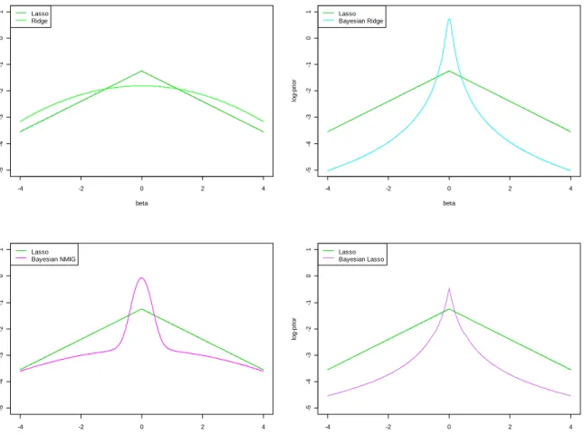
-4 -2 0 2 4 -5 -4 -3 -2 -1 0 1 beta lo g -p rio r Lasso Ridge -4 -2 0 2 4 -5 -4 -3 -2 -1 0 1 beta lo g -p rio r Lasso Bayesian Ridge -4 -2 0 2 4 -5 -4 -3 -2 -1 0 1 beta lo g-pr io r Lasso Bayesian NMIG -4 -2 0 2 4 -5 -4 -3 -2 -1 0 1 beta lo g-pr io r Lasso Bayesian Lasso

Figure 2.1: Log-priors in comparison to the Lasso prior (green line).

2.2.5

Variable selection

Since the Bayesian regularization priors do not share the strong variable selection property of the frequentist Lasso, hard shrinkage rules are considered to accomplish variable selection. A first rule is based on the 95% credible intervals (CI95), obtained from the corresponding sample quantiles of the regression coefficient’s MCMC samples. A second interval criterion is constructed using the sample standard deviation, so that only regression coefficients with zero outside the one standard deviation interval around the posterior mean are included in the final model. On the other hand, the Bayesian NMIG provides a natural criterion to select covariates if the samples of the indicator variables are utilized. Covariates with considerable influence should be assigned to the mixing distribution

component corresponding to the indicator with values ν =₁ 1. The more the posterior mean of an

indicator variable increases (i. e. the percentage of the values ν =₁ 1 in the sample), the larger is the

we use the intuitive cut value of 0.5 as a selection criterion, i. e. covariates whose corresponding indicator posterior mean exceeds 0.5 are included in the final model, see Sections 4 and 5.

2.3

Smoothness priors

Smooth modelling and estimation of nonlinear and time-varying effects including the (log-) baseline hazard, is based on Bayesian P-splines. If we use the partial likelihood for Bayesian inference in model (2.1), no additional prior assumption for the baseline hazard is needed. A justification for using the partial likelihood instead of a genuine likelihood in a Bayesian setting is given in Sinha et al. (2003) for time-constant effects.

A flexible approach to model and to estimate the baseline hazard is to use an approximation with

spline basis functions of degree . To do so, one chooses a sequence of knots ξ < < ξ₁ ... _s from

(

)

( )

( )

M= + −s 1 an appropriate basis of the spline space S

(

)

approximated through

( )

( )

( )

( )

0 0 1 01 M 0M

g t =logλ t =B t γ + +... B t γ .

We can express the predictors as

( )

(

( )

)

(

)

i ti exp log 0 ti xi′ exp zi0′ 0 xi′

η = λ + β = γ + β

with z′ =_i0

(

)

(

)

0 0

Z X

η = γ + β.

To guarantee smoothness for the unknown log baseline hazard g (t) , we assume Bayesian P-spline ₀

priors as in Lang and Brezger (2004). This implies the use of B-spline basis functions of degree to model the log-baseline and first or second order random walk smoothness priors for the parameter

vector γ₀,

0,m 0,m 1− u0,m or 0,m 2 0,m 1− 0,m 2− u0,m

with i.i.d. Gaussian errors 2

0,m 0

u ~ N(0,δ ) and diffuse priors for the initial values π γ( _0,1)∝const or

0,1 0,2

( ) ( ) const.

π γ = π γ ∝ The first order random walk prior controls abrupt jumps in the differences

0,m 0,m 1−

γ − γ , while the second order random walk prior penalizes deviations from a linear trend. The

variance parameter δ2₀ controls the amount of the penalization and acts as a smoothness parameter.

The smaller the variance parameter, the stronger is the penalization. The joint prior for the parameter

0

γ as the product of the conditional densities is

(

)

with penalty matrix K of the form K=D D′ , where D is a first or second order difference matrix and

( )

k=rank K . A standard option for the variance parameter is a diffuse inverse gamma prior

2 0 ~ InvGamma(a , b )0 0 δ with density

(

)

( )

and small a₀>0, b₀ >0. It is also possible to choose an improper Gamma-type prior in the case when

0 0

a ≤0, b ≤0 or especially a₀≤0, b₀ =0, for example a₀ = −0.5, b₀= −1, corresponding to a flat

prior p(δ ∝₀) const for the standard deviation 2

0 0

δ = δ .

In the extended model (2.3), unknown time-varying effects g (t) and nonparametric functions _j f (z ) _{j j}

of continuous covariates are modelled through Bayesian P-splines as well. Let

(

)

j j 1 ij j n ij

g = g (t )v ,...,g (t )v ′ denote the vector of time-varying effects g (t )v and _{j i ni}

(

)

j j ij j ni

f = f (z ),..., f (z ) ′ the vector of evaluations of f (z ) . Then _{j j} g and _j f can be expressed as the _j

product of an appropriately defined design matrix Z and a (possibly) high-dimensional vector _j γ_j of

parameters, for example g_j= γZ_{j j} or f_j= γZ_{j 0}.After reindexing, we can represent the predictor vector

η in generic notation as

0 0 m m

X U Z ... Z

η = β + ζ + γ + + γ ,

see Hennerfeind et al. (2006) for more details and extensions to spatial and group-specific effects. The

j k 2 j j j 2 j j j j 1 p( | ) exp( K ) 2 − _′ γ δ ∝ δ − γ γ δ ,

with precision or penalty matrix K and _j k_j=rank(K ), j_j =0,1,..., m.

3

Posterior inference

We first describe MCMC inference for the basic model (2.2) with predictor η_i(t)=g (t)₀ + βx′_i , where

shrinkage estimates of β, possibly together with a smooth estimate of the log-baseline rate g (t) , are ₀

of interest. Joint shrinkage and smoothing in the extended model (2.3) is outlined subsequently.

3.1

MCMC with shrinkage priors

For inference based on the full likelihood, the posterior has the general form

(

)

(

(

)

)

(

) ( )

(

) ( )

∏

where τ = τ2 ( ,...,₁2 τ_p2) and π τ φ( , )2 is a generic notation for priors defined for τ2 and other parameters

or random variables φ through the hierarchical formulation of shrinkage priors in Section 2.2. Thus,

for all shrinkage priors, the full conditional of the regression parameters β is

( )

(

)

(

)

D_τ=diag τ ,...,τ denotes the matrix of the variance parameters. This distribution has no

closed form to draw a new/proposed state for the Markov chain. We use an MH-algorithm with so-called IWLS-proposals to update the regression coefficients. To do so, the log-likelihood is

approximated by a second order Taylor expansion at the current state of the parameter vector β(c), i. e.

(

)

(

) (

) (

) (

) (

)(

)

(

)

(

)

(

)

with Hessian matrix H_β and score vector s_β. The likelihood is then approximated by a multivariate

(

)

(

)

(

)

The score function is

(

)

(

)

(

)

0 0

l ,

s_β β γ =, ∂ β γ =X d′⎡ − Λ_⎣ t | ,β γ ⎤_⎦

∂β

with Λ

(

)

(

(

)

( )

(

)

(

)

)

(

)

matrix is

(

)

(

)

(

(

)

)

The approximation of the full conditional π β ⋅

( )

(

)

ˆ | ,

π ⋅ β ⋅ with precision and mean

(

)

(

)

(

)

(

(

)

)

is used as the proposal density to draw a new proposal β( )p of the Markov chain which is accepted

with the probability

(

)

(

(

) (

) (

)

)

MH steps for updating the baseline coefficients γ₀ can conceptually be carried out in the same way as

for β, replacing the (conditional) precision matrix _D−1

τ by K /τ20, the precision matrix of the

(conditional) Gaussian prior. However, computational efforts increase because the cumulative baseline hazard is the integral of the baseline hazard involved, complicating derivation and computation of the score function

0

s_γ and the Hessian matrix

0

H_γ . As an alternative, we may use MH steps with

If we rely on posterior inference based on the partial likelihood, we replace the log-likelihood l( ,β γ₀)

through the partial (log-)likelihood pl( )β as well as the score function and Hessian matrix through

corresponding derivatives. The full conditional for β is then given by

( )

( )

and the (partial) score function and Hessian matrix are

( )

( )

(

)

(

)

(

)

(

)

( )

(

)

(

)

(

)

( )

(

)

( )

(

)

(

)

∑

∑

∑

∑

∑

∑

∑

(

)

( )

∑

∑

∑

3.1.1

Bayesian Ridge

The full conditionals for the variance parameters simplify to

2 j 1 | , j 1,.., p. 2 τ ⋅ = = λ

and the full conditional for the shrinkage parameter is a gamma density,

p 2 j j 1 p | Gamma a , b . 2 λ = λ ⎛ ⎞ λ ⋅ _⎜ + β + _⎟ ⎝

∑

3.1.2

Bayesian Lasso

The full conditionals for the variance parameters 2

j, j 1,...p

τ = , and the shrinkage parameter λ2 _are

known densities so that updates for the Markov chain are available via Gibbs steps. The full conditionals for the variance parameters are

( )

m = λ β . Application of the density transformation theorem for 2 2

j 1 j

ω = τ shows that the

full conditional is an inverse Gaussian distribution

2 2 2 j j 1 | InvGauss , , j 1,.., p ⎛ _λ ⎞ ⎜ ⎟ ⋅ λ = ⎜ ⎟ τ ∼ _⎝ β _⎠ .

The full conditional for the quadratic lasso parameter is given as

( ) ( )

∑

∑

3.1.3

Bayesian NMIG

The diagonal matrix D_τ now contains the diagonal elements 2 2

j Ij j

τ = ψ . The full conditionals for the

binary variables indicator variables are

(

)

(

)

( )

( )

(

)

( )

( )

(

)

The full conditionals for the second variance parameter component 2 j

ψ are inverse gamma densities

(

)

The full conditional for the mixing parameter is a Beta density

( )

(

)

( )

( )

( ) (

)

( )

∏

{

}

{

}

(

)

If we use a beta prior we get ω ⋅| ∼Beta a

(

)

3.2

MCMC for jointly shrinking and smoothing

For the extended model (2.3), additional MH steps for drawing from full conditionals for ζ γ, ,...,₁ γ_m

are required. Unpenalized effects ζ are updated again by constructing a Gaussian distribution as

proposal for a new state of the chain via second order Taylor expansion. Proceeding as in Section 3.1,

the Gaussian proposal density π ζ ⋅( | ) has precision and mean

(

)

(

)

(

)

(

(

)

)

A new proposal ζ( )p of the Markov chain is accepted with probability

(

)

(

(

) (

) (

)

)

For a flat prior π ζ ∝( ) const we simply set the precision to _A−1=_0.

Basis coefficients γ_j for functions f (z ) are updated with IWLS proposals as described in _{j j}

Hennerfeind et al. (2006): Given the current state (c)

j

γ , proposals are drawn from a Gaussian density

with precision and mean

(

)

(

)

(

)

(

(

)

)

The full conditionals for the variance parameters 2

j

δ are (proper) inverse Gamma with parameters

1 1

j j 2 j j j 2 j j j

a′ = +a r , b′=b + γ′Kγ .

For the basis coefficients of time-varying effects, it is computationally more efficient to use MH-steps with conditional prior proposals instead of IWLS proposals.

The most costly computation in running the whole MCMC samplers are the inversions of the precision matrices within the IWLS parts of the corresponding parameter vectors. To reduce the running time in the case of high dimensional parameters, a better approach is to update these parameters in blocks of smaller size than the size of the whole parameter vector.

4

Simulations

The performance of the Bayesian Ridge, Lasso and NIG priors, is compared to the frequentist Ridge, Lasso and a backward-stepwise procedure based on the AIC criterion under Cox’s proportional

hazards model. The tuning parameter λ in the frequentist Lasso and Ridge regression is estimated via

n-fold generalized cross validation. The analysis of the parametric and nonparametric models with P-spline and Weibull baseline was done with the free BayesX software available from http://www.stat.uni-muenchen.de/~bayesx/. The partial likelihood based models are carried out with R version 2.6.2 from http://www.r-project.org and are implemented in functions that are available from the authors by request. Frequentistic penalized Lasso and Ridge regression is done in R with the package {penalized}.

In addition to semiparametric modelling of the baseline hazard rate in the Cox model or the P-spline

based approach, we consider a simple parametric Weibull model λ₀

( )

as a competitor. A gamma prior is typically employed to model the prior knowledge about the shape

parameter α, i. e.

(

)

( )

(

)

with E

( )

( )

by the update of α. With the given prior assumption, the full conditional of αis given by

( )

{

( ) (

) ( )

}

{ }

{

}

i i i i

i 1

| exp log 1 log t t exp xα α− exp b

α =

⎡ ′ ⎤

π α ⋅ ∝

∑

To draw a new proposal α(p) _{for the shape parameter we use a Gamma distribution}

(

)

(

)

ˆ | , d_α ~ Gamma d_α , d_α

π ⋅ α α based on the current value α(c) which leads to the acceptance

probability

(

)

(

(

) (

) (

)

)

The value of d_α is determined during the burn in to achieve reasonable acceptance rates.

We measure the estimation accuracy based on the mean squared errors (MSE) over r=50 runs with

sample size n=200 if only linear effects are modelled and n=1000 if nonlinear effects are included

in the predictor. Let V=(X X) / n′ −1 be the population covariance matrix of the regressors, then the

MSE of ˆβ in the r-th simulation replication is given by

( )

(

) (

)

r ˆr ˆr

MSE β = β − β ′V β − β .

For the log-baseline g₀

( )

( )

(

) (

)

where ˆg denotes the vector of estimates of the log-baseline in r-th simulation. To compare the results ₀

likelihood approaches, we use the trapezoidal rule to compute the cumulative baseline hazard.

Concordantly, if f denotes the vector of nonlinear effects of covariate x with estimate ˆf , the MSE is _r

given as

( )

( ) ( )

Additionally, we report the average number of correct and incorrect zero coefficients in the final models achieved after applying one of the hard shrinkage rules discussed in Section 2.2.5.

Simulation settings:

For our first simulations we use the configuration from Tibshirani (1997). The covariates

(

)

i i,1 i,9

x = x ,..., x are randomly drawn from a multivariate Gaussian distribution with zero mean and

covariance matrix chosen such that the correlation between x and _j x is _k co rr x , x

(

)

0.5

ρ = . The survival times T ,i 1,..., n_i = are generated from an exponential hazard model with

constant baseline hazard λ₀

( )

( )

( )

The censoring variables C ,i 1,..., n_i = are generated as i.i.d. draws from the uniform distribution

[

]

U 0,c with c chosen to obtain censoring rates about 25 % in each dataset. For the models ₀

(

)

(

)

(

)

we simulated r=50 datasets with n=200 life times. The first and the second model were used in

Tibshirani (1997) and the third is used in Zhang and Lu (2007). For the Bayesian MCMC methods, we use 10000 iterations with a burnin of 2000 and thin the chain by 8 which results in an MCMC sample of size 1000. The hyperparameters of the Bayesian Lasso and Ridge are set to the low informative

values a_λ =b_λ =0.01 to allow for a greater amount of adaptiveness for the shrinkage parameter

depending on the data. The hyperparameters of the Bayesian NMIG are ν =₁ 1, ν =₀ 0.000025, a_ψ=5

and b_ψ =25. These values are chosen to assign a marginal prior probability of about 0.8 to fall into

the interval [ 2, 2]− to each regression coefficient.

With the subsequent simulations we explore the changes caused by inclusion of a nonlinear effect and more flexible baseline hazards. The settings are similar to those in Hennerfeind et al. (2006). Again we

are generated independently as random draws from a uniform U[ 3,3]− distribution. The lifetimes are generated via the inversion method (Bender, Augustin & Blettner, 2005) from the model

(

)

( )

( )

(

( )

)

The covariates of the linear effects are standardized and the nonlinear effect is centered due to identification arguments leading to an intercept term in the predictor. To model more flexible baseline hazards a linear but non-Weibull baseline hazard of the form

( )

Model 4.a : λ t =0.25+2t

and a bathtub-shaped baseline hazard

( )

(

( )

)

(

)

have been chosen. The latter assumes an initially high baseline risk that decreases after some time and

increases again later on until time t= π2 from where the hazard stays constant. Censoring times are

generated in two steps. First a random proportion of 17% of the generated observations T is assigned _i

to be censored. Then in the second step the censoring times for this random selection are drawn from

the corresponding uniform distributions U 0, T . The hyperparameters for the Bayesian penalties are

[

]

not changed but here we use 20000 iterations with a burnin of 5000 and thin the chain by 10 which results in an MCMC sample of size 1500. Before we describe our results, we introduce some abbreviations to reduce the writing.

B, BT, BL, BN, BR: Bayesian models based on the full likelihood with P-spline baseline hazard without penalization (B), with the predictor that contains only the nonzero effects (BT), with Lasso (BL), NMIG (BN) and Ridge (BR) prior

SURV, SURV.T: Maximum partial likelihood of the full model and the model with the predictor that contains only the nonzero effects

STEP: Partial likelihood model with backward stepwise selection based on AIC Pen.L, Pen.R: Penalized partial likelihood model with Lasso and Ridge penalty

PL.B, PL.BL, PL.BN, PL.BR: Bayesian models based on partial likelihood without penalization (PL.B), with Lasso (PL.BL), NMIG (PL.BN) and Ridge (PL.BR) penalty

WB.B, WB.L, WB.N, WB.R: Bayesian models based on the full likelihood with Weibull baseline hazard without penalization (WB.B), with Lasso (WB.BL), NMIG (WB.BN) and Ridge (WB.BR) penalty

For the Bayesian approaches, the hard shrinkage methods described in Section 2.2.5 are additionally assigned with

HS.CI95: if hard shrinkage is done via the 95% credible region, HS.STD: if hard shrinkage is done via the one standard error region, HS.IND: if hard shrinkage for NMIG is done via indicator variables.

For example, WB.N-HS.IND denotes the Bayesian Weibull model under NMIG penalty when the covariate specific indicators are used to select the covariates for the final model.

4.1

Results for model 1

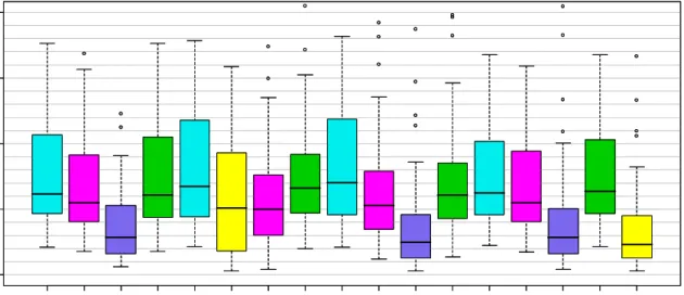
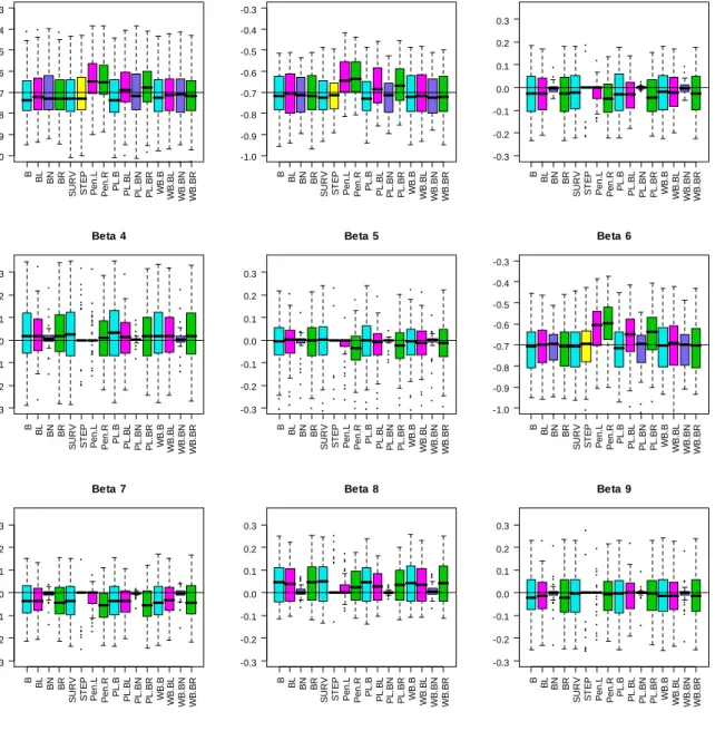
Figure 4.1 shows the box plots of the mean squared errors for the regression coefficients. The Bayesian NMIG performs best within each Bayesian group of models and outperforms the STEP procedure as well as the frequentist and the Bayesian Lasso. The MSEs of the Bayesian NIG are close to the MSE of the maximum partial likelihood estimate if the predictor with the true covariate structure is used (SURV.T). The MSEs of the corresponding unpenalized Bayesian methods are comparable to the MSE of SURV.T and are omitted in the figure. The plots of Figure 4.2 display separate box plots for the corresponding estimated coefficients (except those of STEP.T, which are similar to those of SURV for the nonzero effects). If we focus on the Bayesian methods, we see that the estimates of the NMIG for the truly non-influential coefficients are much more concentrated around zero similar to STEP and Pen.L.

B _BL BN BR S URV _STEP _Pen. L P en. R PL .B PL .BL PL .BN PL .BR WB .B WB .B L WB .B N WB .B R S URV .T 0.00 0.05 0.10 0.15 0.20 B _BL BN BR S URV _STEP _Pen. L P en. R PL .B PL .BL PL .BN PL .BR WB .B WB .B L WB .B N WB .B R S URV .T 0.00 0.05 0.10 0.15 0.20

Figure 4.1: Box plots of the mean squared errors for the regression coefficients of model 1. The right box (SURV.T) shows the MSE for the maximum partial likelihood estimations when the true predictor structure is used.

B BL BN BR S URV _STE P P en. L P en. R PL .B PL .B L PL .B N PL .B R WB .B WB .B L WB .B N WB .B R -1.0 -0.9 -0.8 -0.7 -0.6 -0.5 -0.4 -0.3 Beta 1 B BL BN BR S URV _STE P P en. L P en. R PL .B PL .B L PL .B N PL .B R WB .B WB .B L WB .B N WB .B R -1.0 -0.9 -0.8 -0.7 -0.6 -0.5 -0.4 -0.3 Beta 2 B BL BN BR S URV _STE P P en. L P en. R PL .B PL .B L PL .B N PL .B R WB .B WB .B L WB .B N WB .B R -0.3 -0.2 -0.1 0.0 0.1 0.2 0.3 Beta 3 B BL BN BR S URV _STE P P en. L P en. R PL .B PL .B L PL .B N PL .B R WB .B WB .B L WB .B N WB .B R -0.3 -0.2 -0.1 0.0 0.1 0.2 0.3 Beta 4 B BL BN BR S URV _STE P P en. L P en. R PL .B PL .B L PL .B N PL .B R WB .B WB .B L WB .B N WB .B R -0.3 -0.2 -0.1 0.0 0.1 0.2 0.3 Beta 5 B BL BN BR S URV _STE P P en. L P en. R PL .B PL .B L PL .B N PL .B R WB .B WB .B L WB .B N WB .B R -1.0 -0.9 -0.8 -0.7 -0.6 -0.5 -0.4 -0.3 Beta 6 B BL BN BR S URV _STE P P en. L P en. R PL .B PL .B L PL .B N PL .B R WB .B WB .B L WB .B N WB .B R -0.3 -0.2 -0.1 0.0 0.1 0.2 0.3 Beta 7 B BL BN BR S URV _STE P P en. L P en. R PL .B PL .B L PL .B N PL .B R WB .B WB .B L WB .B N WB .B R -0.3 -0.2 -0.1 0.0 0.1 0.2 0.3 Beta 8 B BL BN BR S URV _STE P P en. L P en. R PL .B PL .B L PL .B N PL .B R WB .B WB .B L WB .B N WB .B R -0.3 -0.2 -0.1 0.0 0.1 0.2 0.3 Beta 9

Figure 4.2: Box plot of the estimated coefficients for the simulation under model 1. The black horizontal lines mark the values of the true effects.

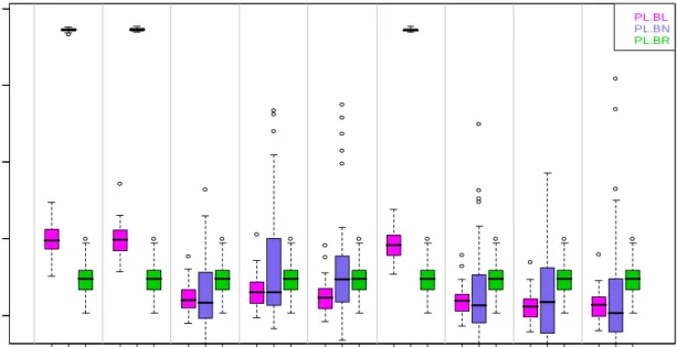
If we take a look at Figure 4.3, we see the different amount of penalization displayed through the box

plots of the logarithm of the variance parameters τ2 for the Bayesian Lasso, Ridge and NMIG

demonstrated on the basis of the partial likelihood. For the nonzero effects β β β₁, ₂, ₆ the corresponding

variance parameters induced by the NMIG penalty take much larger values than those of the Bayesian

Lasso which results in less penalization (1/τ2) of the nonzero coefficients estimates. The variance

parameters of the zero effects are closely comparable. The tendency of small penalization for nonzero effects and larger penalization of zero effects are reflected by both, the Bayesian Lasso and the Bayesian NMIG, but the Bayesian NMIG differences for zero and nonzero effects are larger as those of the Bayesian Lasso.

tau2. x 1 tau2. x 2 tau2. x 3 tau2. x 4 tau2. x 5 tau2. x 6 tau2. x 7 tau2. x 8 tau2. x 9 -2 -1 0 1 2 lo g (Var iances) It2 .x 1 It2 .x 2 It2 .x 3 It2 .x 4 It2 .x 5 It2 .x 6 It2 .x 7 It2 .x 8 It2 .x 9 -2 -1 0 1 2 tau2. x 1 tau2. x 2 tau2. x 3 tau2. x 4 tau2. x 5 tau2. x 6 tau2. x 7 tau2. x 8 tau2. x 9 -2 -1 0 1 2 PL.BL PL.BN PL.BR

Figure 4.3: Box plot of the variance parameters for the Lasso, NMIG and Ridge penalty in the partial likelihood based Bayesian models for model 1.

The variable selection feature of the Bayesian NMIG is highlighted in Figure 4.4 where the box plots

of the relative frequencies of the indicator variables ν =₁ 1 are shown for the partial likelihood and full

likelihood with P-spline baseline. The relative frequencies of the nonzero effects are nearly one with very small standard deviation. For the zero effects, the relative frequencies are shifted towards zero and clearly fall below the selection cut off value of 0.5. Although the frequencies of the full likelihood approach for the zero effects tend to be a little bit higher than those for the partial likelihood, the relative frequencies of the indicator variables seem to provide a good resource to select the important covariates in both cases.

I. x1 I. x2 I. x3 I. x4 I. x5 I. x6 I. x7 I. x8 I. x9 0.0 0.2 0.4 0.6 0.8 1.0 I. x1 I. x2 I. x3 I. x4 I. x5 I. x6 I. x7 I. x8 I. x9 0.0 0.2 0.4 0.6 0.8 1.0 _PL.BN BN

Figure 4.4: Box plot of the relative frequencies of the indicator variables for NMIG penalty if the Bayesian partial likelihood (cyan) and the full likelihood (magenta) with P-spline baseline are used for model 1.

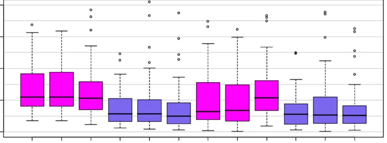
In Figure 4.5, the box plots of the MSE for the regression coefficients are displayed together with the MSE obtained after applying the hard shrinkage criteria for the Bayesian Lasso. The results for the HS.STD criterion are omitted in this figure since they perform worse than the HS.CI95 criterion. The MSE of the Bayesian Lasso tends to be improved, if the hard shrinkage criterion is applied but the performance of the Bayesian NMIG still remains better. Furthermore, the HS.IND criterion only slightly improves the MSE of the Bayesian NMIG since the estimates of the zero effects are very close to zero anyway, i. e. it is negligible if they are removed from the final model. If we take a look on the frequencies of the selected final models, listed for the different hard shrinkage rules in Table 4.1 in column four, we find out, that all hard shrinkage criteria applied to the Bayesian NMIG for all model classes lead to the highest frequencies of the final models with the true nonzero coefficients. The best case of 50 is reached if HS.CI95 is applied, which is here not surprising because the Bayesian NMIG behaves very similar to SURV.T with asymptotic normal estimates. Additionally, the second and third column in Table 4.1 show the average number of the true estimated nonzero coefficients and true estimated zero coefficients for the 50 datasets. All hard shrinkage methods reach the optimal value of three for the true nonzero coefficients. The highest values for the true zero coefficients are again achieved for the Bayesian NMIG.

BL WB .B L PL .B L BN WB .B N PL .B N BL .H S .C I9 5 WB B L .H S .CI 95 PL B L .H S. C I9 5 BN .H S. IN D W BBN .H S. IN D P L BN .H S. IN D 0.00 0.05 0.10 0.15 0.20 BL WB .B L PL .B L BN WB .B N PL .B N BL .H S .C I9 5 WB B L .H S .CI 95 PL B L .H S. C I9 5 BN .H S. IN D W BBN .H S. IN D P L BN .H S. IN D 0.00 0.05 0.10 0.15 0.20

Figure 4.5: Box plot of the Bayesian Lasso (magenta) and NMIG (blue) mean squared errors for the regression coefficients of model 1. The first six boxes compare the methods if inference is based on full likelihood or partial likelihood without hard shrinkage and the last six boxes do the same if additional hard shrinkage is done for the same

models.

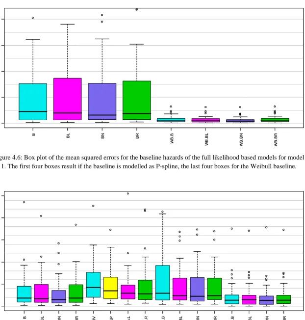
Finally, we take a look at the MSEs of the estimates of the baselines (Figure 4.6) and the cumulative baselines (Figure 4.7) of the different model classes. For the nonparametric baseline modelled via

P-spines and the parametric Weibull model in Figure 4.6 shows that the performance of the Weibull model is better than those of the nonparametric model, which is plausible since the true exponential

baseline is a special Weibull baseline with α =1. A view at the cumulative baselines in Figure 4.7

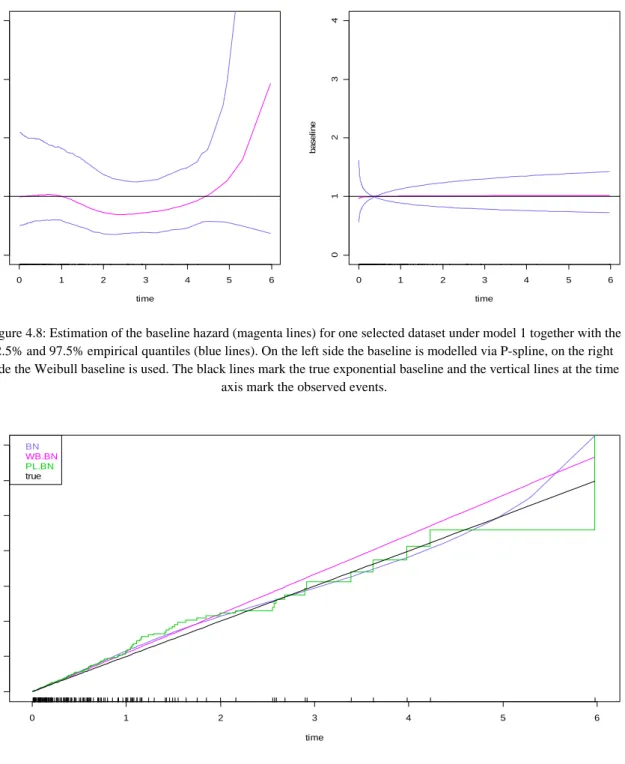
reflects this result again and shows the outperformance of the baseline estimation produced by the full likelihood approaches. In Figure 4.8 and Figure 4.9, we see the estimates of the baseline and cumulative baseline for one selected dataset if Bayesian NMIG is applied. The vertical lines at the

time axis mark the observed events. In the interval [0,1] , where most of the observations occur, the

P-spline baseline approximates the true baseline very well. The deviations get larger, the less observations are available when time increases, which results in an increasing MSE. If we restrict the

calculations of the MSEs to the interval [0,1] the MSEs of the baselines as well as the MSE of the

cumulative baselines of all models are similar.

B _BL BN BR WB .B WB .B L WB .B N WB .B R 0.0 0.2 0.4 0.6 0.8 B _BL BN BR WB .B WB .B L WB .B N WB .B R 0.0 0.2 0.4 0.6 0.8

Figure 4.6: Box plot of the mean squared errors for the baseline hazards of the full likelihood based models for model 1. The first four boxes result if the baseline is modelled as P-spline, the last four boxes for the Weibull baseline.

B BL BN BR S URV _STE P P en. L P en. R PL .B PL .B L PL .B N PL .B R WB .B WB .B L WB .B N WB .B R 0.00 0.05 0.10 0.15 0.20 0.25 B BL BN BR S URV _STE P P en. L P en. R PL .B PL .B L PL .B N PL .B R WB .B WB .B L WB .B N WB .B R 0.00 0.05 0.10 0.15 0.20 0.25

0 1 2 3 4 5 6 01 2 3 4 time b a s e lin e |||||||||||||||||||||||||||||||||||||||||||||||||||||||||||||||||||||||||||||||||||||||||||||||||||||||||||||||||||||||||||||||||| |||||| | | | | | ||| | || | | | | | 0 1 2 3 4 5 6 01 2 3 4 time b a s e lin e |||||||||||||||||||||||||||||||||||||||||||||||||||||||||||||||||||||||||||||||||||||||||||||||||||||||||||||||||||||||||||||||||| ||||||| | | | | ||| | || | | | | |

Figure 4.8: Estimation of the baseline hazard (magenta lines) for one selected dataset under model 1 together with the 2.5% and 97.5% empirical quantiles (blue lines). On the left side the baseline is modelled via P-spline, on the right side the Weibull baseline is used. The black lines mark the true exponential baseline and the vertical lines at the time

axis mark the observed events.

0 1 2 3 4 5 6 0 1 23 45 6 7 time cu m base li n e |||||||||||||||||||||||||||||||||||||||||||||||||||||||||||||||||||||||||||||||||||||||||||||||||||||| |||||||| | || ||||||||||||||| | | |||||| | | | | | ||| | || | | | | | BN WB.BN PL.BN true

Figure 4.9: Cumulative baseline hazards under the Bayesian NIG penalty for one selected dataset under model 1. The black line marks the true exponential cumulative baseline, the vertical lines at the time axis mark the observed events.

4.2

Results for model 2

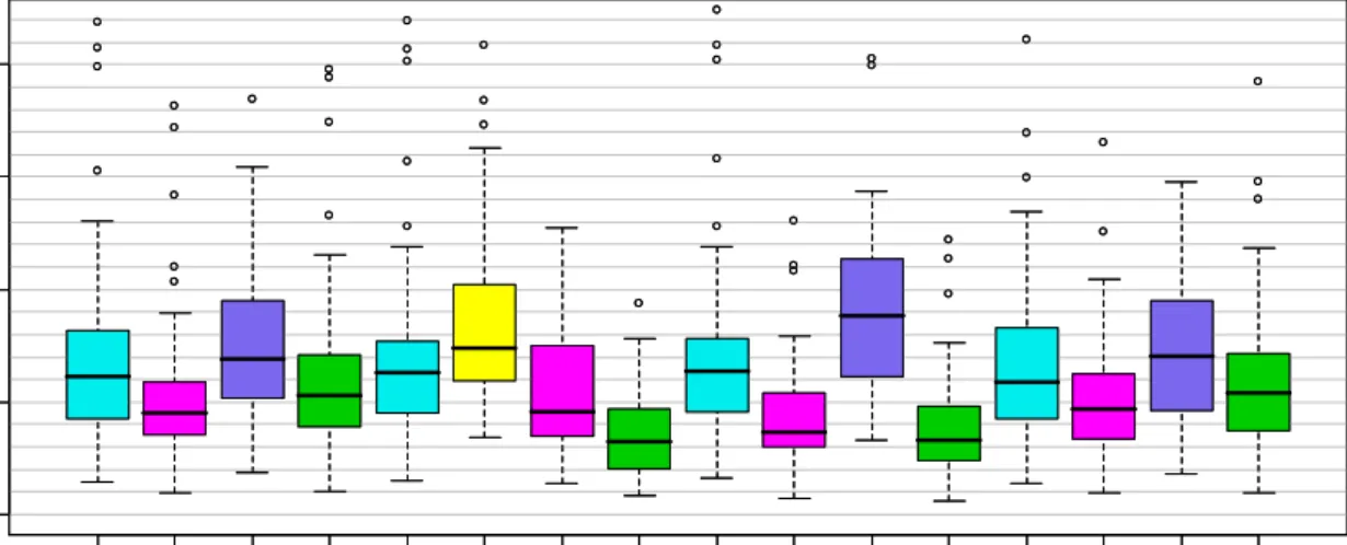
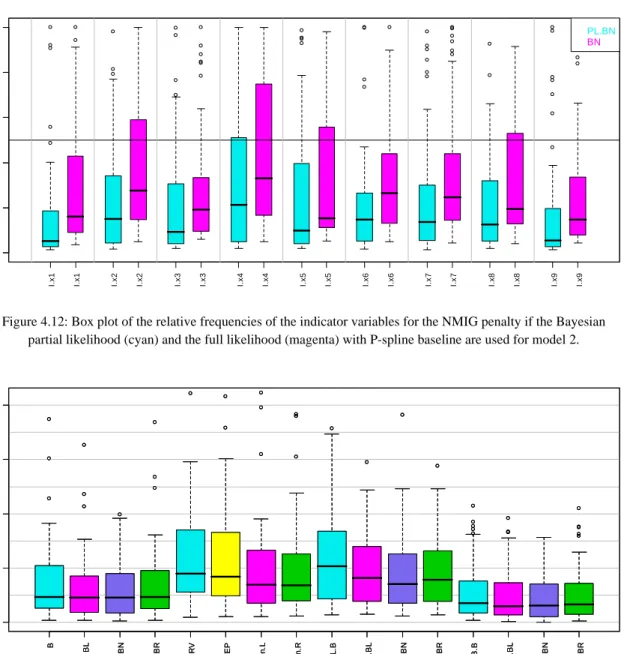
Figure 4.10 shows the MSEs for the different methods if all nine covariates in the predictor are assigned small but nonzero effects. The MSEs for the Bayesian NIG method based on the full likelihood are comparable to the MSE of the stepwise procedure STEP and are larger then the MSEs of the Bayesian Lasso, Ridge and the unpenalized Bayesian approach. The increase of the MSE can be explained when taking a look at Figure 4.12, where the relative frequencies of the indicator variables produced by the Bayesian NMIG penalty are displayed. Almost all relative frequencies of the

indicators are of comparable size and tend to be close to zero, which results in a heavy penalization of all covariates and accordingly in point estimates for the regression coefficients that are very close to zero and don’t reflect the true model. The stepwise procedure behaves similar by producing zero estimates for the small nonzero effects. The best performances are obtained for the Ridge- and Lasso-penalty based methods. It is clear, that in the setting of model 2 with small nonzero effects, the application of the hard shrinkage criteria can not improve the MSE (Figure 4.11). In Table 4.1, the number of correctly identified nonzero and zero estimated coefficients are collected for the hard shrinkage criteria. The best value of nine is reached for none of the approaches. The estimation of the baselines and cumulative baselines leads to comparable results as in model 1 and are summarized in terms of the MSE in Figure 4.13.

B _BL BN BR S URV ST EP P en. L P en. R PL .B PL .B L PL .B N PL .B R WB .B WB .B L WB .B N WB .B R 0.00 0.05 0.10 0.15 0.20 B _BL BN BR S URV ST EP P en. L P en. R PL .B PL .B L PL .B N PL .B R WB .B WB .B L WB .B N WB .B R 0.00 0.05 0.10 0.15 0.20

Figure 4.10: Box plot of the mean squared errors for the regression coefficients of model 2.

BL WB .B L PL .B L BN WB .B N PL .B N BL .H S .C I9 5 WB B L .H S .C I9 5 PL B L .H S. C I9 5 B N .H S .IN D W B B N .H S .IN D PL BN .H S. IN D 0.00 0.05 0.10 0.15 0.20 0.25 BL WB .B L PL .B L BN WB .B N PL .B N BL .H S .C I9 5 WB B L .H S .C I9 5 PL B L .H S. C I9 5 B N .H S .IN D W B B N .H S .IN D PL BN .H S. IN D 0.00 0.05 0.10 0.15 0.20 0.25

Figure 4.11: Box plot for the Bayesian Lasso (magenta) and NMIG (blue) mean squared errors for the regression coefficients of model 2. The first six boxes compare the methods if inference is based on full likelihood or partial likelihood without hard shrinkage, while the last six boxes correspond to results when additional hard shrinkage is

I. x1 I. x2 I. x3 I. x4 I. x5 I. x6 I. x7 I. x8 I. x9 0.0 0.2 0.4 0.6 0.8 1.0 I. x1 I. x2 I. x3 I. x4 I. x5 I. x6 I. x7 I. x8 I. x9 0.0 0.2 0.4 0.6 0.8 1.0 _PL.BN BN

Figure 4.12: Box plot of the relative frequencies of the indicator variables for the NMIG penalty if the Bayesian partial likelihood (cyan) and the full likelihood (magenta) with P-spline baseline are used for model 2.

B BL BN BR SU R V ST E P Pe n .L P en. R PL .B PL .B L PL .B N PL .B R WB .B WB .B L WB .B N WB .B R 0.00 0.02 0.04 0.06 0.08 B BL BN BR SU R V ST E P Pe n .L P en. R PL .B PL .B L PL .B N PL .B R WB .B WB .B L WB .B N WB .B R 0.00 0.02 0.04 0.06 0.08

Figure 4.13: Box plot of the mean squared errors for the cumulative baseline hazards of model 2.

4.3

Results for model 3

Figure 4.14 shows the MSEs achieved in the estimation of model 3. Again, the MSEs of the maximum partial likelihood estimators for the true predictor structure are recorded as a benchmark result. The penalty based approaches achieve lower MSEs than those without penalisation and the best MSEs are derived with the Lasso penalty in combination with the partial likelihood. The performance of the full likelihood based methods are similar if the Lasso and NMIG penalty are employed. Taking a look at

Figure 4.15 where the relative frequencies of the value ν =₁ 1 of the Bayesian NMIG are displayed,

reveals that the relative frequency for the largest effect with value -0.4 is nearly 1 and for the second largest effect with value -0.2 the cut off value of 0.5 is frequently passed over. Further simulations (not

presented in this work) have shown that effects with absolute values larger than 0.3 can be separated from the zero effects very we