Working Paper No. 61
Modelling zero-inflated count data when
exposure varies:
with an application to sick leave
Gregori Baetschmann and Rainer Winkelmann
February 2012
University of Zurich
Department of Economics
Working Paper Series
ISSN 1664-7041 (print)
ISSN 1664-705X (online)
Modelling zero-inflated count data when
exposure varies:
with an application to sick leave
∗
Gregori Baetschmann
Department of Economics, University of Zurich
Rainer Winkelmann
Department of Economics, University of Zurich, CESifo and IZA
February 2012
Abstract
This paper is concerned with the analysis of zero-inflated count data when time of exposure varies. It proposes a new zero-inflated count data model that is based on two homogeneous Poisson processes and accounts for exposure time in a theory consistent way. The new model is used in an application to the effect of insurance generosity on the number of absent days.
JEL Classification: J29, C25
Keywords: exposure, Poisson regression, complementary log-log link
∗Address for correspondence: University of Zurich, Department of Economics, Z¨urichbergstr. 14, CH-8032
Z¨urich, Switzerland, phone: +41 44 634 22 95 and +41 44 634 22 92, email: [email protected]
1
Introduction
This paper is concerned with conditional probability models for count data when the proportion
of zeros in the empirical distribution exceeds that predicted by the two standard approaches, the
Poisson and the negative binomial regression models. Such “excess zeros” are frequently present in
health related research. The main recommendation in the literature (see e.g. Jones, 2007, B¨ohning
et al., 1997) is to use a class of modified count data models that is referred to as “zero-inflated”,
and indeed, applications of the zero inflated Poisson and negative binomial models are abundant
(Pizer and Prentice, 2011; Sari, 2009; Sarma and Simpson, 2006; Yen, Tang and Su, 2001; Chang
and Trivedi, 2003; Street, Jones and Furuta, 1999).
The key feature of these models is the presence of two types of zeros, “normal” zeros and “extra”
zeros. Lambert (1992), in the context of manufacturing defects, refers to the latter as resulting
from a “perfect state”, in contrast to the count process zeros that represent an “imperfect state”
where events occur without being inevitable. A related distinction is that between “strategic” and
“incidental” zeros. For example, when modelling the number of physician visits, a person might
have had zero visits during a given time period because (i) she is a follower of alternative medicines
and never visits a doctor, or because (ii) she visits doctors in principle but by chance did not do so
during the observed period.
The main objective of this paper is to study the effect of varying exposure in such zero inflated
count data models. For simplicity, we equate exposure with “period-at-risk”, i.e. time, although
other interpretations, for example a spatial one, are possible without altering the substantial
argu-ments and conclusions. Varying exposure can be of interest for two main reasons. First, it might be
to a different time frame. For example, a health survey may collect information on the number of
doctor visits during a 3-months reference period, whereas the real outcome of interest is the annual
number of visits. Second, exposure may differ between units of observation. In this case, ignoring
exposure effects in modelling and estimation will in general lead to spurious effect estimates.
In either case, a crucial issue is how exposure affects the extra zeros. At one end of the spectrum,
the probability of an extra zero does not depend on exposure time at all. This assumption leads to
proportionality between the expected number of counts and exposure, and it is implicitly made in
most existing applications of count data models with logit-type zero inflation. We argue that this
assumption is not very plausible. At a minimum, it should be tested. When the null-hypothesis of
no time-dependence of extra zeros is rejected, one requires, for estimation as well as extrapolation, a
model of time dependence. A natural benchmark model is one where the extra zeros are generated
from a homogeneous Poisson process and the expected number of events is therefore proportional
to exposure time. The probability of an extra zeros is then equal to the survivor function of the
exponential distribution, and the distribution model is a Bernoulli distribution withcomplementary
log-log link (cloglog). Thus, we propose a new zero-inflated count data model where the usual logit
assumption for the extra zeros is replaced by that of a cloglog function. This modification allows
us to account, and test, for time of exposure effects in a theory-consistent way.
The paper proceeds as follows. In the next section, we show that, within the context of a
zero-inflated model, increased exposure is in general not compatible with a proportional effect of
exposure on the expected number of counts. In section 3, we discuss the limitations of an existing
proposal to introduce varying exposure times into zero inflated count data models, and present a
new model that addresses these limitations. In section 4, the new approach is applied to the effect
2
Zero-inflated count models and exposure
The zero-inflated Poisson model with covariates but ignoring exposure can be written as (see e.g.
B¨ohning et al., 1997, Winkelmann, 2008)
Pr(y|x, z) = ω(z) + (1−ω(z)) exp(−λ(x)) for y= 0 (1−ω(z))exp(−λ(x))λ(x) y y! for y= 1, 2, 3, . . .
where y is a count-valued random variable and ω ∈ [0,1] is a zero-inflation parameter. Typically,
λ(x) = exp(x0β) and ω(z) is specified as a logit, such that
ω(z) = exp(z
0γ)
1 + exp(z0γ) (1)
where x and z can be disjunct, overlapping, or identical. It follows from this double index
specifi-cation that
E(y|x, z) = (1−ω)λ= exp(x
0β)
1 + exp(z0γ) (2)
whereωandλare defined for a given exposuret. The model parameters can either be estimated
by maximum likelihood, or by exploiting moment restrictions derived from (2) (e.g, using nonlinear
least squares or Poisson pseudo maximum likelihood, see Staub and Winkelmann, 2011).
It is straightforward to modify the zero-inflated Poisson model in order to allow for overdispersion
in addition to zero-inflation. Suppose that there is unobserved heterogeneity such that λ(x, u) =
λ(x)u. If u follows a gamma distribution with E(u|x) = 1 and Var(u|x) = 1/α, and if y conditional onx anduis Poisson distributed with expectation λ(x)u, then the distribution ofy, conditional on
xbut unconditional on u, is negative binomial with parameters λ(x) and α.
Lee et al. (2001) propose an extension of the model to account for varying exposure. Suppose
that
but that the probability of an extra zero is unaffected by exposure time. In this case, (2) can be
re-written as
E(y|x, z, t) =t exp(x
0β)
1 + exp(z0γ)
and the conditional expectation is proportional to exposure time by construction. Alternatively,
one can let λ(x, t) = exp(x0β+αlogt) = tαexp(x0β) and test whether α = 1. Clearly, neither of
the two approaches is entirely satisfactory because both are based on the assumption that only the
parent process is affected by exposure time, whereas the proportion of extra zeros is time-invariant.
3
A new zero-inflation model with varying exposure
Suppose that both ω =ω(t) and λ =λ(t) are functions of time. In general, we would expect that
the probability of an extra zero decreases with the amount of exposure, and thatω0(t)<0. From
E(y(t)) = (1−ω(t))λ(t),
(where the dependence on x and z is suppressed for simplicity) it follows that
dE(y(t))
dt =−ω
0
(t)λ(t) + (1−ω(t))λ0(t)
Even if the effect in the parent model is proportional to time of exposure (λ(t) = λt and
λ0(t) = λ), the overall effect is not proportional since
dE(y(t))
dt =−ω
0
(t)λt+ (1−ω(t))λ
The expected value of a zero-inflated count model increases proportionally with exposure only
with increasing exposure, then ω0(t)λt ≤ 0 and the expected value of such a zero-inflated count model increasesoverproportionally as a function of exposure.
This has practical consequences. Returning to our initial example, it is not possible to use
results regarding the mean number of quarterly doctor visits and extrapolate to an annual rate,
as this would require a proportionality assumption that may be invalid. If, instead, ω0(t) < 0,
this kind of extrapolation based on proportionality underestimates the annual rate. There is
an-other consequence of assuming ω0(t) = 0 when in fact it is not. Suppose, a log-linear conditional
expectation function λ(x) = exp(x0β) has been specified, and the interest is in estimating β, the
semi-elasticities. Without proportionality, the estimates are not invariant to exposure time: a
re-searcher using observations from a longer observation period will obtain estimates that differ from
a researcher using a shorter period. Clearly, this is unwanted.
A meaningful modelling approach should account for these problems and estimate ω0(t) from
data, rather than imposing a value and sign a-priori. For such an estimation-based approach,
there are two requirements. First, one needs to observe variation in exposure time across units of
observation. Without such variation, the effect of exposure cannot be identified. Second, one needs
to specify a meaningful model forω(t).
In principle, one could include some arbitrary function of tas a regressor in the logit model (1).
Alternatively, and in our view preferably, one should introduce exposure effects on extra zeros in a
theory driven way, based on a stochastic process that generates these additional zeros. Suppose that
this process is a Poisson process with rateµ. Then an extra zero for exposure periodt is obtained
if the duration until the first event exceeds t. In a Poisson process, the duration is exponentially
thereby obtain the complementary log-log (cloglog) model with exposure:
ω(z, t) = exp(−exp(z0γ+ logt)) (4)
Using ˜ω = exp(−exp(z0γ+δlogt)) instead, we can test for proportionality in the underlying Poisson process (i.e.,δ= 1), just as was the case for the Poisson part of the model. Ifδ = 0, the extra zeros
are time-invariant and hence truly “strategic”. The parametersγ measure the effect of a regressor
on the underlying hazard function. A positive γ means that an increase in the associated variable
increases the hazard rate and therefore reduces the probability of an extra zero.
The log-likelihood function of the Poisson-cloglog model for zero inflated count data, based on
a sample of n independent observations on yi, xi and zi, can be written as
X
yi=0
ln[exp(−µi) + exp(−λi)−exp(−µi−λi)] +
X
yi>0
ln[1−exp(−µi)]−λi+yilnλi
where λi and µi are defined as in (3) and (4), respectively. The EM algorithm has been shown to
work well in this kind of problem, but straight Newton-Raphson maximization is possible as well.
The log-likelihood function for the negative binomial-cloglog model can be obtained accordingly. For
testing, it should be noted that neither do zero-inflated models nest their standard parent models,
nor have the logit and cloglog specifications for the extra zeros a nested structure. Thus testing
therefore needs to follow procedures developed for non-nested models, as discussed for example in
Vuong (1989).
4
Application
We re-analyze the dataset and model of Barmby, Nolan and Winkelmann (2001). They studied
binomial regression models without accounting for extra zeros. The data stem from a manufacturing
firm operating a production line. Employees are contracted to work either 4 or 5 days a week, where
4 day workers do not necessarily work fewer weekly hours. Thus it is possible to estimate the effect
of an additional weekly work day on absence, keeping overall working hours constant. Workers
are entitled to company sickpay. There is some experience rating, as the sickpay depends on the
average number of yearly absent days, calculated over the last two years. Workers with less then 10
days of absence are graded with an A and are entitled to replacement of basic earnings plus bonus.
Workers with a grade B (between 10 and 20 absent days) are entitled to replacement of basic pay,
while employees with grade C (more than 20 absent days) receive only the statutory sickpay level.
A detailed discussion of economic models of absence behavior can be found in Treble and Barmby
(2011).
The number of weekly working days is proportional to exposure-time, since period-at-risk is
equal to the number of weekly working days times number of weeks in the observation period (52
weeks minus vacation periods). Thus, exposure of workers with a 5 days contract is 25 percent
higher than that of 4 days workers. If nothing else was going on, one would therefore expect that
5 day workers have 25 percent more absent days than 4 day workers. If λ(x, t) is specified as
exp(x0β+γlog(days)) and if the absentee counts are proportional to exposure-time, the estimated
effect of log(days), ˆγ should not statistically differ from 1. Of course, the number of contracted
workdays might have other effects on absenteeism. First, it is important to realize that the insurance
scheme awards grades based on the absolute number of days absent rather than the rate. Thus the
system is relatively more generous for people contracted for 4 days a week: they can have a higher
absenteeism rate than 5 day workers, but still keep the same or a higher grade. Second, it is
preferences, and that the two types differ in their inherent absence rates. Both factors can mean
that the exposure effect departs from proportionality, something that can be tested in the present
application.
Barmby, Nolan and Winkelmann (2001) discussed this issue in the context of a negative binomial
(negbin) model. Here, we generalize their analysis by considering a zero inflated negative binomial
model (which results from the assumption of a Poisson process gamma distributed heterogeneity for
the parent distribution). The motivation of using a zero inflated count data instead of an ordinary
negbin model in this application is the high proportion of people without any absent days (15%
of the sample), whereas the mean of the variable is equal to 7.8 and the variance is 67. Hence, in
addition to an ordinary negbin model, a zero inflated Poisson and a zero inflated negative binomial
model are estimated and tested against each other. As described in the previous part, a cloglog link
is used to model excess zeros, and the logarithm of contracted workdays is included as a regressor in
both parts of the model. Thus, if work day status does not affect the rate of the excess zero process,
the parameter of log(days) should also be 1 in the inflated part of the model. Beside log(days) and
dummies for grade B and C, the model includes a female dummy, the wage rate, and the average
daily working hours. These are the same variables as in Barmby, Nolan and Winkelmann (2001).
− − − −Table 1 about here− − − −
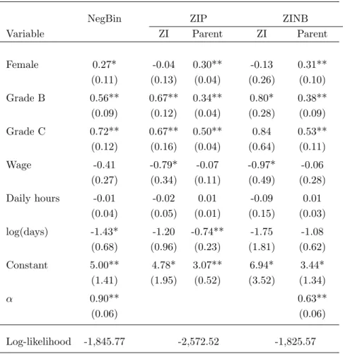
Results of the three models are shown in Table 1. The value of the Vuong-test-statistic of
the inflated negbin against the negbin model without excess zeros is 3.04 (p-value < 0.01) and
hence suggests the existence of additional zeros. A likelihood ratio test of the two processes with
excess zeros clearly prefers the zero-inflated negbin model over the zero-inflated Poisson model (test
excess zero process (results are available upon request). Although the model with cloglog link has
the largest log likelihood value compared to the models with logit or probit link, the differences
are minor. In the following, we concentrate our discussion on the zero inflated negbin model with
cloglog link (ZINB in Table 1).
The way the models are specified, a positive coefficient means that an increase in the associated
regressor shifts the incidence rate of the underlying Poisson processes upward. Such a shift increases
the expected number of absent days in the count part, and it decreases the number of excess zeros.
Thus, if the coefficients in the two parts of the model have the same sign, the effects go in the same
direction, indicating, for instance, that the overall conditional expectation (2) is moved in the same
direction. In this application, with two exceptions, coefficients in the inflated model have the same
sign as in the parent process.
As in Barmby, Nolan and Winkelmann (2001), a strong effect of sickpay status is present in the
parent model. In addition, we find a similar effect for the inflated part. People with a grade B or C
have thus not only a higher expected number of absent days, but they also have fewer excess zeros
(compared to similar people with grade A).
Regarding work day status, the effects are opposite to what one would expect: not only are five
day workers no more absent than four day workers, despite their higher exposure, but they are even
less so, based on point estimates at least. The point estimates associated with log(days) can be
interpreted as elasticities: a one percent increase in exposure (the number of contracted workdays)
is predicted to lower the number of absent days in the parent process by 1.1 percent, and to lower
the rate in the strategic zero process by 1.75 percent. For example, with a 10% probability of an
extra zero, the rate would fall from 2.3 = −ln 0.1 to 2.26, which translates into a .4 percentage point increased probability of such a zero. While we would need a larger sample to actually reject
the null hypothesis of no effect (i.e., that these zeros are truly “strategic” and do not depend on
exposure), we find these point estimates telling per-se.
Our methodology suggests an alternative test, namely one of the natural benchmark under
varying exposure, that of proportionality. Under that scenario, the rates for workers with 5 day
contracts should lie 25% above those of workers with 4 day contracts, since the period-at-risk is
correspondingly higher. In our model, this means a coefficient of 1 for log(days) in both processes.
Note that such a direct benchmarking is not possible in any of the other standard zero-inflated
count data models. Individually, the hypothesis that the log(days) coefficient is equal to 1 can be
rejected in the parent part but not so in the excess zero part. However, if we test the proportionality
hypothesis jointly, it is rejected (at the 1% level of significance).
This somewhat counterintuitive finding calls for an explanation. Part of the higher absenteeism
rate of 4 day workers can be explained by the relative generosity of the sickpay scheme, since the
thresholds are formulated as absolute number of days, not in relative terms. While the relatively
generous treatment of 4 day workers can explain a higherrate, it still remains a puzzle why they even
have a higher total absence count. Most likely, work day status is correlated with other unobserved
characteristics, which by themselves affect the absenteeism rate.
5
Conclusions
The paper shows how to extend zero inflated count data models if exposure-time varies and affects
the parent as well as the inflated part of the model. This generalizes an approach by Lee et al.
(2001) where exposure time was only allowed to affect the parent process. Under the assumption
to parameterize the excess zeros. As in the Poisson process, this allows to adjust for varying
period-at-risk in a theory consistent way, by including the logarithm of exposure-time as an additional
control variable in the inflated part of the model. A constant shrinking rate of excess zeros then
implies a coefficient of 1 for the effect of log(exposure-time), which can be tested.
A re-examination of Barmby, Nolan and Winkelmann (2001) about the effect of insurance scheme
on sick leave days reveals the presence of excess zeros depending on period-at-risk. Thus five day
workershave not only a lower absenteeism rate than four day workers, they have also an increased
probability of having no absent days. Further, their lower absenteeism rate more than offsets the
extended period-at-risk. Therefore, the number of counts in the observation period is even lower for
five day workers. Work day status is thus probably correlated with other unobserved characteristics
affecting the two rates. In addition, we find that sickpay status has a strong effect in the parent
as well as in the inflated model and in general, variables seem to affect both rates in the same
direction. The application shows that the zero inflated negative binomial model can be adapted for
varying exposure-time in the same way as the zero inflated Poisson model.
6
References
Barmby, T., M. Nolan and Winkelmann, R. (2001), Contracted workdays and absence,Manchester
School, 69(3), 269-275.
B¨ohning, D., Dietz, E. and Schlattmann, P. (1997), Zero-inflated count models and their
applica-tions in public health and social science. In: Rost, J. and Langeheine, R. (Eds.), Application
of Latent Trait and Latent Class Model in Social Sciences. Wasemann, M¨unster, 333-344.
(1999), The Zero-Inflated Poisson Model and the Decayed, Missing and Filled Teeth Index in
Dental Epidemiology, Journal of the Royal Statistical Society. Series A (Statistics in Society),
162(2), 195-209.
Chang, Fwu-Ranq and Pravin K. Trivedi (2003), Economics of Self-Medication: Theory and
Evi-dence, Health Economics, 12, 721-739.
Jones, A. (2007), Applied econometrics for health economists: a practical guide, 2nd ed., Radcliffe
Publishing.
Lee, Andy H., Kui Wang and Kelvin K. W. Yau (2001), Analysis of Zero-Inflated Poisson
Incor-porating Extent of Exposure, Biometrical Journal, 43(8), 963-975.
Pizer, Steven D., and Julia C. Prentice (2011), Time Is Money: Outpatient Waiting Times and
Health Insurance Choices of Elderly Veterans in the United States, Journal of Health
Eco-nomics, 30, 626-636.
Sari, Nazmi (2009), Physical Inactivity and its Impact on Healthcare Utilization, Health
Eco-nomics, 18, 885-901.
Sarma, Sisira, and Wayne Simpson (2006), A microeconometric analysis of Canadian health care
utilization, Health Economics, 15, 219-239.
Staub, Kevin E., and Rainer Winkelmann (2011), Consistent estimation of zero-inflated count
models, University of Zurich Socioeconomic Institutes Working Paper SOI 0908.
Street, Andrew, Andrew Jones and Aya Furuta (1999), Cost sharing and pharmaceutical utilisation
Treble, John and Tim Barmby (2011) Worker Absenteeism and Sick Pay, Cambridge University
Press.
Yen, Stephen T., Chao-Hsiun Tang and Shew-Jiuan B. Su (2001), Demand for Traditional Medicine
in Taiwan: A Mixed Gaussian-Poisson Model Approach, Health Economics, 10, 221-232.
Vuong, Quang H. (1989), Likelihood Ratio Tests for Model Selection and non-nested Hypotheses,
Econometrica, 57(2), 307-333.
Table 1: Effect of insurance scheme on absent days
NegBin ZIP ZINB
Variable ZI Parent ZI Parent
Female 0.27* -0.04 0.30** -0.13 0.31** (0.11) (0.13) (0.04) (0.26) (0.10) Grade B 0.56** 0.67** 0.34** 0.80* 0.38** (0.09) (0.12) (0.04) (0.28) (0.09) Grade C 0.72** 0.67** 0.50** 0.84 0.53** (0.12) (0.16) (0.04) (0.64) (0.11) Wage -0.41 -0.79* -0.07 -0.97* -0.06 (0.27) (0.34) (0.11) (0.49) (0.28) Daily hours -0.01 -0.02 0.01 -0.09 0.01 (0.04) (0.05) (0.01) (0.15) (0.03) log(days) -1.43* -1.20 -0.74** -1.75 -1.08 (0.68) (0.96) (0.23) (1.81) (0.62) Constant 5.00** 4.78* 3.07** 6.94* 3.44* (1.41) (1.95) (0.52) (3.52) (1.34) α 0.90** 0.63** (0.06) (0.06) Log-likelihood -1,845.77 -2,572.52 -1,825.57
Notes: Dependent variable: absent days. 604 observations. Number of Zeros: 90. Standard errors in parentheses. **, * denote statistical significance at the 1%, 5%,
significance levels, respectively. αindicates the overdispersion parameter of the
neg-ative binomial type II distribution. Vuong test of ZINB against NegBin: z= 3.04,