Bayesian mixture models for count data

(1)

Glasgow Theses Service http://theses.gla.ac.uk/

[email protected]

Chanialidis, Charalampos (2015)

Bayesian mixture models for count

data.

PhD thesis.

http://theses.gla.ac.uk/6371/

Copyright and moral rights for this thesis are retained by the author

A copy can be downloaded for personal non-commercial research or study, without prior permission or charge

This thesis cannot be reproduced or quoted extensively from without first obtaining permission in writing from the Author

The content must not be changed in any way or sold commercially in any format or medium without the formal permission of the Author

When referring to this work, full bibliographic details including the author, title, awarding institution and date of the thesis must be given

(2)

Charalampos Chanialidis

A Dissertation Submitted to the University of Glasgow

for the degree of Doctor of Philosophy

School of Mathematics & Statistics

November 2014

c

(3)

Regression models for count data are usually based on the Poisson distri-bution. This thesis is concerned with Bayesian inference in more flexible models for count data. Two classes of models and algorithms are presented and studied in this thesis. The first employs a generalisation of the Pois-son distribution called the COM-PoisPois-son distribution, which can represent both overdispersed data and underdispersed data. We also propose a den-sity regression technique for count data, which, albeit centered around the Poisson distribution, can represent arbitrary discrete distributions. The key contribution of this thesis are MCMC-based methods for posterior inference in these models.

One key challenge in COM-Poisson-based models is the fact that the nor-malisation constant of the COM-Poisson distribution is not known in closed form. We propose two exact MCMC algorithms which address this problem. One is based on the idea of retrospective sampling; we sample the uniform random variable u used to decide on the acceptance (or rejection) of the proposed new state of the unknown parameter first and then only evaluate bounds for the acceptance probability, in the hope that we will not need to

(4)

know the acceptance probability exactly in order to come to a decision on whether to accept or reject the newly proposed value. This strategy is based on an efficient scheme for computing lower and upper bounds for the nor-malisation constant. This procedure can be applied to a number of discrete distributions, including the COM-Poisson distribution. The other MCMC algorithm proposed is based on an algorithm known as the exchange algo-rithm. The latter requires sampling from the COM-Poisson distribution and we will describe how this can be done efficiently using rejection sampling. We will also present simulation studies which show the advantages of using the COM-Poisson regression model compared to the alternative models com-monly used in literature (Poisson and negative binomial). Three real world applications are presented: the number of emergency hospital admissions in Scotland in 2010, the number of papers published by Ph.D. students and fertility data from the second German Socio-Economic Panel.

COM-Poisson distributions are also the cornerstone of the proposed density regression technique based on Dirichlet process mixture models. Density regression can be thought of as a competitor to quantile regression. Quan-tile regression estimates the quanQuan-tiles of the conditional distribution of the response variable given the covariates. This is especially useful when the dis-persion changes across the covariates. Instead of estimating the conditional mean _E(Y|X = x), quantile regression estimates the conditional quantile function QY(p|X = x) across different quantiles p where p ∈ (0,1). As a result, quantile regression models both location and shape shifts of the conditional distribution. This allows for a better understanding of how the covariates affect the conditional distribution of the response variable. Almost

(5)

all quantile regression techniques deal with a continuous response. Quantile regression models for count data have so far received little attention. A tech-nique that has been suggested is adding uniform random noise (“jittering”), thus overcoming the problem that, for a discrete distribution, QY(p|X =x) is not a continuous function of the parameters of interest. Even though this enables us to estimate the conditional quantiles of the response variable, it has disadvantages. For small values of the response variable Y, the added noise can have a large influence on the estimated quantiles. In addition, the problem of “crossing quantiles” still exists for the jittering method. We eliminate all the aforementioned problems by estimating the density of the data, rather than the quantiles. Simulation studies show that the proposed approach performs better than the already established jittering method. To illustrate the new method we analyse fertility data from the second German Socio-Economic Panel.

Keywords: Quantile regression; Bayesian nonparametrics; Mixture models; COM-Poisson distribution; COM-Poisson regression, Markov chain Monte Carlo.

(6)

I know that I lack the writing skills to explain within a couple of sentences how I feel about my supervisors, Ludger and Tereza, but I will give it a try. Your patience, support, and guidance throughout these three years has been astounding. I can’t think of a better pair of supervisors for a Ph.D. student to have. Thanks for putting up with me.

I am deeply grateful to all the people in the department. You are one of the (many) reasons why I will never forget my time in Glasgow.1 _{I have}

to personally thank Beverley, Dawn, Jean, Kathleen, and Susan for their assistance over the years. I am pretty sure I have emailed you more times than what I have Ludger and Tereza together. A lot of thanks should also go to the academic staff of the department for providing a friendly environment for all the Ph.D. students. On a more personal note, I want to thank Agostino, Adrian, Dirk, and Marian for reasons that I would convey to them next time we meet.

I have made some really good friendships in Glasgow during the years. I feel really lucky that I had the opportunity to get to know Andrej, Chari,

1_{Living in Maryhill for a year is another reason.}

(7)

Daniel, Gary, Helen, Kathakali, Lorraine, Maria, and Mustapha among oth-ers. Thanks for all the laughs, discussions, and fun we have had.

Thanks should also go to people that have never set foot on Glasgow but still manage to be there for me: Irina for all the transatlantic skype meetings we have had and are still having,2 _{Grammateia and Thanos for all their help}

throughout the years, and finally my family for the same reasons that I have already explained in my M.Sc. thesis.3

Declaration

I have prepared this thesis myself; no section of it has been submitted previ-ously as part of any application for a degree. I carried out the work reported in it, except where otherwise stated.

2_{Not letting me use the word} _relish_{on my post-doctoral application proved helpful.}

(8)

Abstract i

Acknowledgements iv

List of Figures xi

List of Tables xviii

1 Introduction 1

1.1 Overview of methods . . . 1

1.2 Thesis organisation . . . 7

1.3 Contributions . . . 8

2 Review of background theory 9

2.1 Distributions for count data . . . 9

(9)

2.1.1 Poisson distribution . . . 9

2.1.2 Negative binomial distribution . . . 11

2.1.3 COM-Poisson distribution . . . 14

2.1.4 Other distributions . . . 20

2.2 Regression models for count data . . . 27

2.2.1 Poisson regression . . . 31

2.2.2 Negative binomial regression . . . 32

2.2.3 COM-Poisson regression . . . 33

2.2.4 Other regression models . . . 34

2.3 Quantile regression . . . 37

2.4 Mixture models . . . 46

2.4.1 Finite mixture model . . . 46

2.4.2 Dirichlet distribution . . . 49

2.4.3 Dirichlet process . . . 50

2.4.4 Dirichlet process mixture model . . . 52

2.4.5 Flexibility of the COM-Poisson mixture model . . . 56

(10)

2.5.1 Stochastic simulation . . . 63

2.5.2 MCMC diagnostics . . . 65

2.6 Bayesian density regression for continuous data . . . 67

2.6.1 Dunson et al. model . . . 67

2.6.2 Weighted mixtures of Dirichlet process priors . . . 70

2.6.3 Importance of location weights . . . 71

2.6.4 Generalised P´olya urn scheme . . . 72

2.6.5 MCMC algorithm . . . 75

2.6.6 Clustering properties . . . 77

2.6.7 Predictive density and simulation examples . . . 78

2.6.8 Other approaches to density regression . . . 84

3 Simulation techniques for intractable likelihoods 86 3.1 Intractable likelihoods . . . 87

3.2 Retrospective sampling in MCMC . . . 88

3.2.1 Piecewise geometric bounds . . . 92

3.2.2 MCMC for retrospective algorithm . . . 100

(11)

3.3.1 Algorithm . . . 102

3.3.2 Efficient sampling from the COM-Poisson distribution . 105 3.3.3 MCMC for exchange algorithm . . . 107

3.4 Simulation study comparing the algorithms. . . 108

4 Flexible regression models for count data 113 4.1 COM-Poisson regression . . . 114

4.1.1 Model . . . 114

4.1.2 Shrinkage priors . . . 115

4.1.3 MCMC for COM-Poisson regression . . . 118

4.2 Bayesian density regression for count data . . . 122

5 Simulations and case studies 128 5.1 Simulations . . . 129

5.1.1 COM-Poisson regression . . . 129

5.1.2 Bayesian density regression . . . 134

5.2 Case studies . . . 150

5.2.1 Emergency hospital admissions . . . 150

(12)

5.2.3 Fertility data . . . 176

6 Conclusions and future work 194

Appendices 199

A MCMC diagnostics 200

A.1 COM-Poisson regression . . . 202

A.2 Bayesian density regression. . . 208

B (More) Simulations 214

(13)

2.1 Quantile regression lines forp∈ {0.05,0.1,0.25,0.5,0.75,0.9,0.95}

and mean regression line. . . 41

2.2 Quantile regression curves forp∈ {0.05,0.1,0.25,0.5,0.75,0.9,0.95}

and mean regression curve. . . 44

2.3 Graphical representation of the finite mixture model. . . 47

2.4 One random draw for the probability weights for 100

observa-tions for α= 1,5,10. . . 53

2.5 Graphical representation of the Dirichlet process mixture model. 54

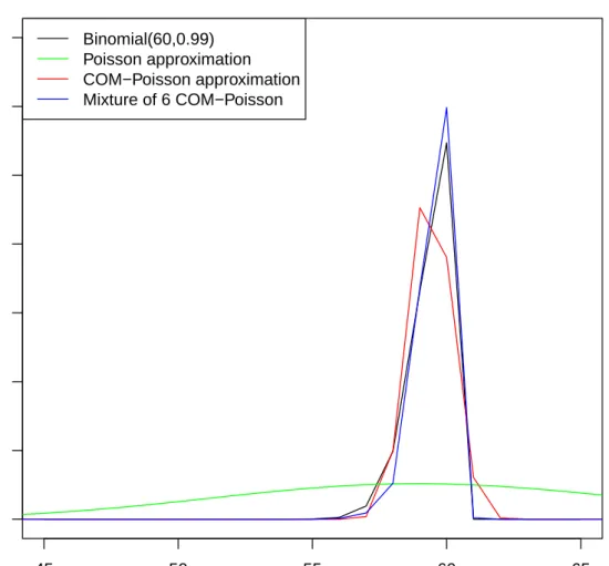
2.6 Approximating a binomial distribution with large mean and

small variance. . . 59

2.7 Approximating a geometric distribution. . . 60

2.8 Drawback of choosing a Dirichlet process as a mixing

distri-bution. . . 70

(14)

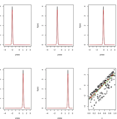
2.9 True conditional densities ofy|xand posterior mean estimates

(example with more covariates). . . 80

(example with non-constant variance). . . 81

(for a mixture model). . . 83

3.1 Illustration of the retrospective sampling algorithm (panels b

and c) in contrast to the standard Metropolis-Hastings

algo-rithm (panel a). . . 92

3.2 Computing the lower and upper bounds of the normalisation

constant in blocks of probabilities. . . 96

3.3 Bounds for the normalisation constant Z(µ, ν) for different

values of µ and ν. . . 99

3.4 Trace plots and density plots forµ andν using the

retrospec-tive MCMC. . . 110

3.5 Trace plots and density plots for µ and ν using the exchange

MCMC for n = 100. . . 110

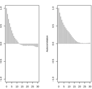
3.6 Autocorrelation plots forµandνusing the retrospective MCMC

for n= 100. . . 111

3.7 Autocorrelation plots forµ and ν using the exchange MCMC

(15)

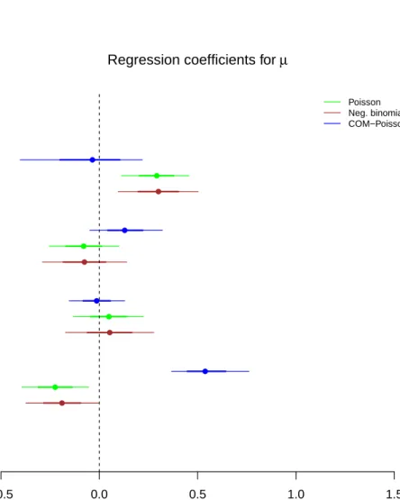
5.1 Simulation: 95% and 68% credible intervals for the regression

coefficients of µ. . . 132

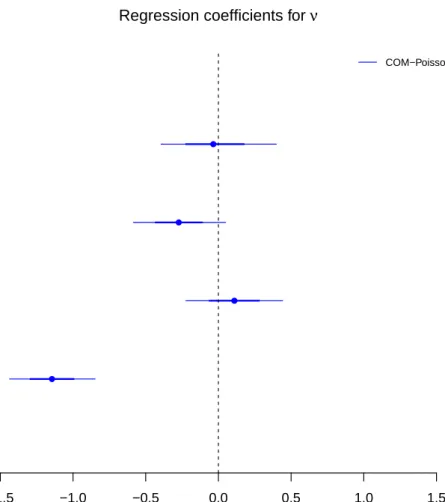
5.2 Simulation: 95% and 68% credible intervals for the regression

coefficients of ν. . . 133

for count data (for a COM-Poisson model). . . 138

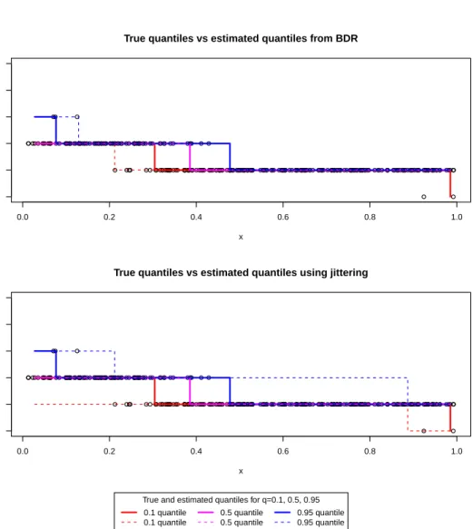
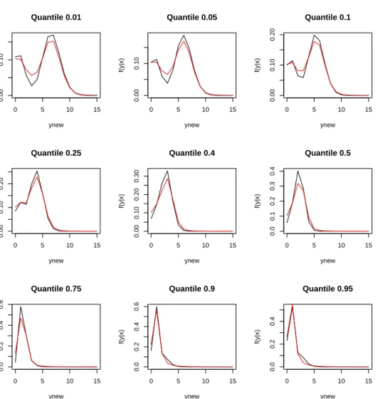
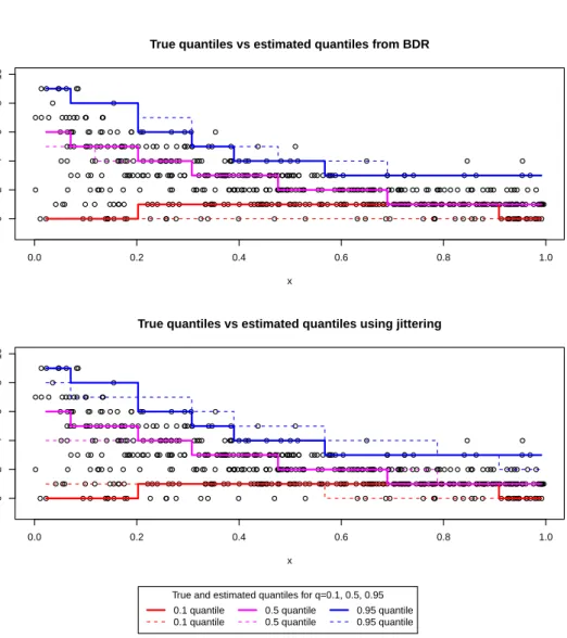
5.4 True quantiles vs estimated quantiles from jittering and Bayesian

density regression.. . . 139

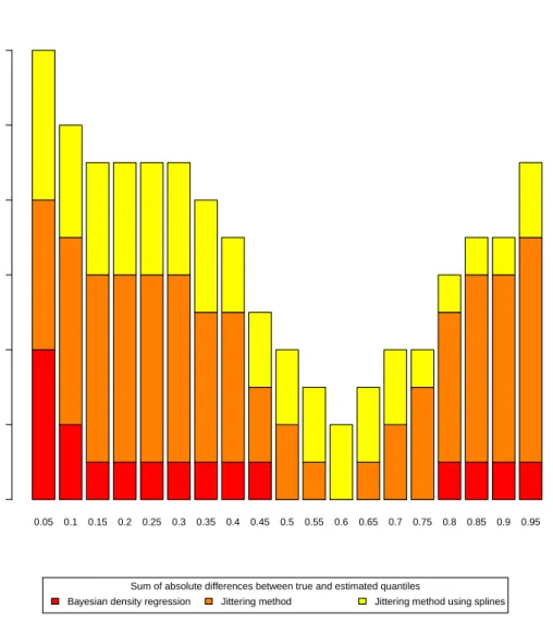
5.5 Sum of absolute differences between true and estimated

quan-tiles across the covariate space. . . 140

for count data (for a mixture model). . . 141

density regression.. . . 142

for count data (binomial distribution) . . . 144

(16)

for count data (mixture of distributions with different

disper-sion levels) . . . 147

density regression . . . 148

5.15 Credible intervals for the regression coefficients of µ for the

local authorities of Scotland. . . 163

5.16 Credible intervals for the regression coefficients of ν for the

local authorities of Scotland. . . 164

5.17 Credible intervals for the regression coefficients forµ for each

class of the Scottish government’s urban/rural classification. . 165

5.18 Credible intervals for the regression coefficients for ν for each

class of the Scottish government’s urban/rural classification. . 166

5.19 SIR for emergency hospital admissions. . . 167

5.20 Publication data: 95% and 68% credible intervals for the

(17)

5.21 Publication data: 95% and 68% credible intervals for the

re-gression coefficients ofν. . . 175

5.22 Fertility data: 95% and 68% credible intervals for the

regres-sion coefficients of µ. . . 179

5.23 Fertility data: 95% and 68% credible intervals for the

regres-sion coefficients of ν. . . 180

5.24 Sample and predicted relative frequencies for the number of

children. . . 182

children. . . 183

children. . . 184

children. . . 185

children. . . 186

children. . . 187

(18)

children. . . 192

A.1 Trace plots forβ1, β2, β3, β4. . . 202

A.2 Trace plots forβ5, β6, β7, β8. . . 203

A.3 Trace plots forc1, c2, c3, c4. . . 204

A.4 Trace plots forc5, c6, c7, c8. . . 205

A.5 Number of clusters across iterations. . . 209

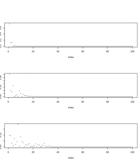
A.6 Cumulative mean probabilities for each value of y (in colour) along with the true probabilities (in grey) fory= 0,1, . . . ,15,

for xi1 = 0.25. . . 211

A.7 95% highest posterior density intervals for the estimated prob-abilities . . . 212

A.8 KL divergence between the true probability distribution and the cumulative means of the estimated probabilities . . . 213

B.1 True conditional densities ofy|xand posterior mean estimates for count data (for a mixture model) . . . 216

B.2 True quantiles vs estimated quantiles from jittering and Bayesian density regression . . . 217

(19)

B.3 True conditional densities ofy|xand posterior mean estimates

for count data . . . 218

B.4 True quantiles vs estimated quantiles from jittering and Bayesian

(20)

2.1 Overview of some well known discrete distributions. . . 13

2.2 Overdispersed count data distributionsfY(y) along with their

mixing distributionsfγ(γ), where f(y|γ) has a Poisson

distri-bution. . . 26

2.3 Link and mean functions of some common distributions. . . . 30

2.4 Quantile functions of the exponential, Pareto, uniform and

logistic distributions. . . 38

3.1 Summary statistics for both parameters and both MCMC

al-gorithms (for n= 10,100,1000). . . 112

5.1 Integrated mean absolute error obtained using the different

density/quantile regression methods. . . 137

5.2 Levels of income deprivation in Scotland’s 15% most deprived

areas.. . . 152

(21)

5.3 The local share considers the percentage of a local authority’s

datazones that are amongst the 15% most deprived in Scotland.153

5.4 The local share considers the percentage of a local authority’s

datazones that are amongst the 15% least deprived in Scotland.154

5.5 Scottish Government joint urban/rural classification. . . 155

5.6 Posterior medians of the non-model-based regression

coeffi-cients for each local authority. . . 160

5.7 Posterior medians for the regression coefficients of the full model.161

5.8 Posterior medians for the variance and spatial autocorrelation

of the random effects. . . 162

5.9 Percentages for refinements when updating the parameter µ. . 168

5.10 Percentages for refinements when updating the parameter ν. . 168

5.11 Mean values for the difference of the log bounds and the

com-puted terms when updating the parameter µ. . . 169

5.12 Mean values for the difference of the log bounds and the

com-puted terms when updating the parameter ν.. . . 170

5.13 Description of variables. . . 171

5.14 Description of variables. . . 176

5.15 Deviance information criterion for all models (minimum DIC

(22)

5.16 DIC and WAIC for the fertility data (minimum criterion is in

bold). . . 190

5.17 Kullback-Leibler divergence between the predicted

distribu-tions and the observed distribution. . . 193

A.1 Autocorrelation for coefficients ofβ at lags= 1,5,10,50. . . 206

A.2 Autocorrelation for coefficients ofc at lags= 1,5,10,50. . . 207

(23)

Introduction

1.1

Overview of methods

Quantile regression was first proposed by Koenker and Bassett (1978) as a more robust method to outliers compared to the classic linear regression (least squares regression). Since then it has been applied in areas such as economics (e.g. effects of union membership on wages (Chamberlain, 1994), hedge fund strategies (Meligkotsidou et al., 2009)), educational reform (e.g. effects of reducing class size on students (Levin, 2001)) and public health (e.g. pollution levels on upper quantiles (Lee and Neocleous, 2010)) among many others. One reason for the popularity of quantile regression is that it allows us to explore the entire conditional distribution, including the tails, of the response variable given the covariates. Thus, we can focus on the lower tail of the distribution if we are interested in poverty studies (which concern the low-income population) and on the upper tail if we are interested

(24)

in tax-policy studies that usually concern the high-income population. In addition, if the assumptions made in least-squares regression such as Gaus-sianity or homoscedasticity do not hold, then, by just looking at the changes to the mean, we may under/overestimate or even fail to see what is happening to the conditional distribution of the response variable. Unlike least squares regression, where all inferences depend on the estimated parameter ˆβ, quan-tile regression allows us to be more precise since the estimated parameters ˆβ_p

depend on the quantile p. Quantile regression can suffer from the problem of “crossing quantile” curves, which is usually seen in sparse regions of the covariate space. This happens due to the fact that the estimated conditional quantile curve for a given X =x is not necessarily a monotonically increas-ing function of p. This is a notable problem of quantile regression, for which there exists no general solution. Koenker (1984) considers parallel quantile planes in order to avoid the “crossing quantiles” problem. He (1997) and

Wu and Liu (2009) propose methods to estimate the quantile curves while

at the same time ensuring that they will be non-crossing. This problem also affects nonlinear quantile curves where different methods for solving it have been proposed. More information is given by Dette and Volgushev (2008);

Chernozhukov et al. (2009,2010) and Bondell et al. (2010).

Most quantile regression techniques deal with a continuous response. The problem with applying quantile regression to count data is that the distribu-tion of the response variable is not continuous. As a result, the quantiles are not continuous either, and they cannot be expressed as a continuous function of the covariates. Machado and Santos Silva (2005) overcome this problem by adding uniform random noise (“jittering”) to the counts. The general

(25)

idea is to construct a continuous variableZ whose conditional quantiles have a one-to-one relationship with the conditional quantiles of the counts Y and use this for inference. After estimating the conditional quantiles of Z we can now use the previous relationship to get the conditional quantiles of the counts Y. This approach eliminates the problem of having a non-continuous distribution for the response variable, but it has the drawback that for small values of Y the estimated conditional quantiles QY(p|X = x) will not be good estimates of the true conditional quantiles. This approach has been applied in the analysis of traffic accidents in Qin and Reyes (2011) and Wu

et al.(2014), frequency of individual doctor visits inWinkelmann(2006) and

Moreira and Barros (2010), and fertility data in Miranda (2008) and Booth

and Kee (2009).

We overcome both aforementioned problems (“jittering” whenY takes small values and the “crossing quantiles” problem) by estimating the conditional density1 _{of the response variable and by obtaining the quantiles through}

the density. The Bayesian density estimation methods that we will follow throughout the thesis are based on Dirichlet process models, which are also known as infinite mixture models. The idea behind mixture models is that the observed data cannot be characterised by a single distribution but instead by several; with the distribution used for a given observation chosen at random. In a sense we treat a population as if it consists of several subpopulations. We can apply these models to data where the observations come from different groups and the group memberships are not known, but also to represent

1_{The word “density” will be used both for the probability mass function in the discrete}

(26)

multimodal distributions. An infinite mixture model can be thought of as

a mixture model with a countably infinite number of components. It is

different to a finite mixture model because it does not use a fixed number of components to model the data. The number of components can be inferred from the data using the Bayesian posterior inference scheme. Neal (2000) proposes different ways for sampling from the posterior of a Dirichlet process model.

In order to be able to estimate any form of conditional density, we assume that the conditional distribution of the countsY can be expressed as a Dirich-let process mixture of regression models where the mixing weights vary with covariates. The weights are dependent on the distance between the values of the covariates as proposed byDunson et al.(2007) when considering Bayesian methods for density regression. Density regression is similar to quantile re-gression in that it allows flexible modelling of the response variable Y given the covariates X =x. Features (mean, quantiles, spread) of the conditional distribution of the response variable vary with X, so, depending on the pre-dictor values, features of the conditional distribution can change in a different way than the population mean. The difference between density regression and quantile regression is that density regression models the probability den-sity function rather than directly modelling the quantiles. Specifically, we will assume that the conditional distribution of the counts can be expressed as a Dirichlet process mixture of COM-Poisson regression models.

The Conway-Maxwell-Poisson (or COM-Poisson) distribution was first pro-posed inConway and Maxwell(1962) in the context of queuing systems with state-dependent service rates and brought back to surface by Shmueli et al.

(27)

(2005). Due to its extra parameter, compared to the Poisson distribution, it is flexible enough to handle any kind of dispersion. The main reason why the COM-Poisson is not used as much in practice is that its normalisation constant is not available in closed form and approximations to it are ei-ther computationally inefficient or not sufficiently exact. In the context of COM-Poisson mixtures, we overcome this problem by resorting to an MCMC strategy, known as the exchange algorithm (Murray et al., 2006). The key idea of the exchange algorithm is to introduce auxiliary data, which allows cancelling out the normalisation constants which are difficult to compute. To recap, we will estimate the conditional density by bridging:

i) an MCMC algorithm for sampling from the posterior distribution of a Dirichlet process model, with a non-conjugate prior, found in Neal

(2000).

ii) The MCMC algorithm in Dunson et al. (2007).

iii) A variation of the MCMC exchange algorithm of Murray et al.(2006).

Besides the above implementation of Bayesian density regression, we will also focus on the COM-Poisson regression model. Shmueli et al. (2005) describe methods for estimating the parameters of the COM-Poisson distribution and show its flexibility in fitting count data compared to other distributions. The advantage of this model is that it allows separation between a covari-ate’s effect on the mean of the counts and on the variance of the counts. The disadvantage is, as we have already mentioned, that the normalisation constant has to be approximated. Minka et al. (2003) provide an

(28)

asymp-totic approximation that is only reasonably accurate in some parts of the parameter space.

We propose an exact MCMC algorithm that is based on the idea of retrospec-tive sampling found in Papaspiliopoulos and Roberts (2008), and compute lower and upper bounds for the acceptance probability of the Metropolis-Hastings MCMC algorithm. The basic idea is that there is not always a need to know the acceptance probability of the MCMC exactly. Often we can make a decision (accept/reject) only based on lower and upper bounds for the acceptance probability. We will also show how one can sample from the COM-Poisson distribution and thus use the exchange algorithm for posterior inference in COM-Poisson regression models.

In Chapter 5 we will demonstrate this method using data on emergency

hospital admissions in Scotland in 2010 where the main interest lies in the estimation of the variability of admissions, as it is considered a proxy for health inequalities. The COM-Poisson regression model is an ideal model for this data set, since it allows modelling the mean and the variance explicitly. As a result, we are able to identify areas with a high level of health inequal-ities. Furthermore, the results show that in order for the MCMC to make a decision between accepting or rejecting a move, the approximation of the bounds of the acceptance probability does not, usually, need to be precise.

(29)

1.2

Thesis organisation

Chapter 2provides a literature review of distributions for count data, regres-sion models for count data, quantile regresregres-sion, mixture models, Dirichlet processes, Bayesian inference and Bayesian density regression models, which all form the background theory needed for the understanding of the thesis. Chapter 3introduces the proposed simulation techniques for intractable like-lihoods, based on retrospective sampling and the exchange algorithm, and presents the MCMC algorithms for each one.

Chapters4and5are each split into two sections; the first section is related to the COM-Poisson regression model while the other is related to the Bayesian density regression model. These refer to the regression models (Chapter 4), and simulations and case studies (Chapter 5) for each model. The thesis is structured in this way for two reasons: to show the similarities and differences between the models, and to make it an easier read for people who are mainly interested in a specific topic.

(30)

1.3

Contributions

The work presented in Chapter 3 (Section 3.2) and Chapter 5 (Section 5.2) has been published in Stat with the title Retrospective MCMC sampling with an application to COM-Poisson regression (Chanialidis et al., 2014) and was presented at the 1st _{International Conference of Statistical Distributions and} Applications.

The work presented in Chapter 3 (Section 3.3) and Chapter 5 (Section 5.2) has been submitted for publication with the titleEfficient Bayesian inference for COM-Poisson regression models.

The work presented in Chapter 4 has been published in the Proceedings of the 21st _{International Conference on Computational Statistics with the title}

Bayesian density regression for count data and was presented at the above conference and the 2nd _{Bayesian Young Statisticians conference.}

All the above contributions can be found on my website.2

(31)

Review of background theory

2.1

Distributions for count data

2.1.1

Poisson distribution

Count data are typically used to model the number of occurrences of an event within a fixed period of time. Examples of count data may include

• the number of goals scored by a team.

• the number of telephone connections to a wrong number.

• the number of murders in a city.

The Poisson distribution is the most popular model used for modelling a discrete random variable Y. It is used to describe “rare” events and it is derived under three assumptions.

(32)

1. The probability of one event happening in a short interval is propor-tional to the length of the interval.

2. The number of events in non-overlapping intervals is independent, and 3. the probability of two events happening in a short interval is negligible

in comparison to the probability of a single event happening.

The probability mass function of the Poisson(µ) distribution is P(Y =y|µ) = exp{−µ}µ

y

y! y= 0,1,2, . . . (2.1)

The mean and variance of a Poisson(µ) are respectively

E[Y] =µ,

V[Y] =µ. (2.2)

The equations in (2.2) show that the Poisson distribution assumes that the mean is equal to its variance; this is known as the equidispersion assumption. This assumption also implies that the Poisson distribution does not allow for the variance to be adjusted independently of the mean. In the presence of underdispersed data (variance is less than the mean) or overdispersed data (variance is greater than the mean) the Poisson distribution is not an appropriate model and one has to use another parametric model, with an additional parameter compared to the Poisson. For overdispersed data, one of the distributions that may provide a better fit is the negative binomial distribution.

(33)

2.1.2

Negative binomial distribution

The probability mass function of the negative binomial(r, p) distribution is P(Y =y|r, p) =py(1−p)r y+r−1 y y= 0,1,2, . . . (2.3)

The mean and variance of a NB(r, p) are respectively

E[Y] = pr

(1−p),

V[Y] = pr

(1−p)2. (2.4)

An alternative formulation of the negative binomial distribution is

P(Y =y|µ, k) = Γ( 1 k +y) Γ(1_k)y! kµ 1 +kµ y 1 1 +kµ 1_k (2.5)

with mean and variance for the negative binomial(µ, k)

E[Y] =µ,

V[Y] =µ+kµ2. (2.6)

The first parameter of this formulation is the mean of the distribution whereas the second is referred to as the dispersion parameter. Large values of k are a sign of overdispersion, while when k → 0 the variance of the distribution (cf. (2.6)) is equal to the mean and we have the Poisson model as a special case.

The negative binomial distribution can also be seen as a continuous mixture of Poisson distributions in which the mixing distribution of the Poisson pa-rameter µ follows a gamma distribution. In this way, we treat the Poisson parameter µas a random variable and we assign to it a gamma distribution.

(34)

Later, in 2.1.4, we will see that there are a plethora of choices for the mixing distribution. Suppose that y ∼Poisson(µ), µ∼gamma(a, b). (2.7) Then f(y) = Z ∞ 0 f(y, µ) dµ = Z ∞ 0 f(y|µ)f(µ) dµ = Z ∞ 0 exp{−µ}µ y y! ba Γ(a)µ a−1_exp_{−_bµ_} _dµ = b a Γ(a) µy y! Z ∞ 0 µy+a−1exp{−(b+ 1)µ} dµ = b b+ 1 a 1 b+ 1 y Γ(y+a) Γ(y+ 1)Γ(a). (2.8)

which is the probability mass function of a negative binomial(r, p) with

p= b

1 +b, r=a. (2.9)

Equations (2.6) show that the negative binomial cannot model underdis-persed data. Some well-known discrete distributions are summarised in Table

(35)

Bernoulli distribution Y = 1 if ev en t A = { success } o ccurs θ probabilit y of success E [ Y ] = θ Ry = { 0 , 1 } Y = 0 otherwise V [ Y ] = θ (1 − θ ) P (0) = 1 − θ ,P (1) = θ Binomial distribution n um b er of successes in indep enden t Bernoulli trials n n um b er of Bernoulli trial s E [ Y ] = nθ Ry = { 0 , 1 ,. .. ,n. } (sampling with replacemen t from p opulation of typ e I θ probabilit y of success V [ Y ] = nθ (1 − θ ) P ( Y = y | n, θ ) = n y θ y(1 − θ ) n − y (prop ortion θ ) and typ e II (prop ortion 1 − θ ) ob jects) Geometric distribution n u m b er of indep enden t trials requ ired un til first θ probabilit y of success E [ Y ] = 1 1 − θ RY = N failure o ccurs E [ Y ] = θ (1 − θ ) 2 P ( Y = y | θ ) = θ y − 1(1 − θ ) P oisson distribution n um b er of ev en ts in time in terv al µ a v er age n um b er of ev en ts E [ Y ] = µ RY = N 0 V [ Y ] = µ P ( Y = y | µ ) = exp {− µ } µ y y ! Negativ e binomial distribution n um b er of successes in in dep enden t Bernoulli trials r n um b er of failures E [ Y ] = pr (1 − p ) RY = N 0 b efore a sp ecified n um b er of failures o ccur p probabilit y of success V [ Y ] = pr (1 − p ) 2 P ( Y = y | r, p ) = p y(1 − p ) r y + r − 1 y T able 2.1: Ov erview of some w ell kno wn discrete distribution s.

(36)

2.1.3

COM-Poisson distribution

The COM-Poisson distribution (Conway and Maxwell,1962) is a two-parameter generalisation of the Poisson distribution that allows for different levels of dispersion. The probability mass function of the COM-Poisson(λ, ν) distri-bution is P(Y =y|λ, ν) = λ y (y!)ν 1 Z(λ, ν) y= 0,1,2, . . . Z(λ, ν) = ∞ X j=0 λj (j!)ν, (2.10) for λ >0 and ν≥0.

The additional parameterν, compared to the Poisson distribution, allows the COM-Poisson distribution to model underdispersed (ν > 1) or overdispersed (ν < 1) data. The Poisson distribution is a special case (ν = 1). The ratio of two successive probabilities is

P(Y =y−1) P(Y =y) =

yν

λ . (2.11)

The range of possible values ofνcovers all different kinds of dispersion levels. Values ofν less than one correspond to flatter successive ratios compared to the Poisson distribution. This means that the distribution has longer tails (e.g. overdispersion). On the other hand, when ν is greater than one, we have underdispersion.

The COM-Poisson distribution is a generalisation of other well known dis-crete distributions:

(37)

• For ν= 1 the distribution is a Poisson(λ).

• For ν→ ∞ it approaches a Bernoulli(_λλ₊₁) distribution.

For ν 6= 1 the normalisation constant Z(λ, ν) does not have a closed form and has to be approximated.

Evaluating the normalisation constant Z(λ, ν)

Minka et al. (2003) give an upper bound for the normalisation constant and

an asymptotic approximation which is reasonably accurate for λ >10ν_{. The} upper bound on Z(λ, ν) is estimated using the fact that the series ₍_jλ_!)jν

con-verges and lim

j→∞

λj (j!)ν = 0.

As a result there exists a value k such that, for j > k, λ

jν <1. (2.12)

This ratio is monotonically decreasing, which means that for j > k, this series converges faster than a geometric series with multiplier given by (2.12).

Minka et al. (2003) truncate the series at the kth _{term such that}

Z(λ, ν) = k X j=0 λj (j!)ν +Rk, (2.13) where Rk= ∞ X j=k+1 λj (j!)ν (2.14)

is the absolute truncation error.

The absolute truncation error Rk is bounded by λk+1

(k+ 1)!ν₍₁₋

k)

(38)

wherekis such that ₍_j₊₁₎λ ν < kfor all j > k. A computational improvement that increases efficiency is to bound the relative truncation error given by

Rk k X j=0 λj (j!)ν . (2.16)

For ν ≤ 1, truncation of the infinite sum is costly since there is a large number of summations needed in order to achieve sensible accuracy. In that case, Minka et al. (2003) use an asymptotic approximation forZ(λ, ν),

Z(λ, ν) = exp{νλ 1 ν} λν2−ν1(2π) ν−1 2 √ ν(1 +O(λ −1_ν )). (2.17)

The formula in (2.17) has been derived for integerν. The main message from this formula is that the normalisation constant Z(λ, ν) grows rapidly as λ increases or ν decreases.

Estimating the COM-Poisson parameters

Shmueli et al. (2005) describe three methods for estimating the parameters

of the COM-Poisson distribution and show its flexibility in fitting count data compared to other distributions.

1. The first method is based on equation (2.11). Taking a log of both sides of the equation

log P(Y =y−1) P(Y =y) =−log{λ}+νlog{y}. (2.18) The ratio on the left hand side can be estimated by replacing the prob-abilities with the relative frequencies of y−1 and y respectively. One

(39)

can plot these values versus log{y} for all the ratios that do not in-clude the zero counts. A COM-Poisson would be an adequate model if the points fall on a straight line. If the data do appear to fit a COM-Poisson model, the parameters can be estimated by fitting a regression of lognP_P(Y₍_Y=₌y−_y₎1)o on log{y}.

2. The second method is based on the maximum likelihood approach. The likelihood for a set of n independent and identically distributed observations y1, y2, . . . , yn is L(y1, y2, . . . , yn|λ, ν) = Qn i=1λyi Qn i=1(yi!)ν Z(λ, ν)−n =λS1_exp_{−_νS 2}Z(λ, ν)−n. (2.19) where S1 =Pn_i₌₁yi and S2 =Pn_i₌₁log{yi!}.

Equation (2.19) shows that (S1, S2) are sufficient statistics fory1, y2, . . . , yn, and that the COM-Poisson is a member of the exponential family since it can be expressed in the form

L(y|θ) =γ(θ)φ(y) exp ( _k X j=1 πj(θ)tj(y) ) (2.20) where y= (y1, y2, . . . , yn)| and θ = (λ, ν).

For the COM-Poisson case

π1(θ) = log{λ}, π2(θ) =−ν, t1(y) = n X i=1 yi, t2(y) = n X i=1 log{yi!}. (2.21) 3. The third method is based on Bayesian inference, see Section 2.5 for more information on Bayesian inference. This approach takes advan-tage of the exponential family structure of the COM-Poisson distribu-tion to establish a conjugate family of priors. Kadane et al. (2006)

(40)

show that the conjugate prior density of the COM-Poisson distribution is of the form:

h(λ, ν) = λa−1exp{−bν}Z−c(λ, ν)k(a, b, c) (2.22)

forλ >0 andν ≥0, wherek(a, b, c) is the normalisation constant. The posterior then is of the same form, with

a0 =a+S1, b0 =b+S2, c0 =c+n. (2.23) The conjugate prior can be thought of as an extended bivariate gamma distribution. In order for equation (2.22) to constitute a density, it must be non-negative and integrate to one. The values of a, b, c that lead to a finite k(a, b, c)−1_{, which is given by}

k(a, b, c)−1 = Z ∞ 0 Z ∞ 0 λa−1exp{−bν}Z−c(λ, ν) dλ dν, (2.24)

will lead to a proper density. A necessary and sufficient condition for equation (2.22) to constitute a density is

b c >log n ba cc o +a c − b a cc logna c + 1 o (2.25)

where bkcdenotes the floor function which returns the highest integer smaller than, or equal to, k. Estimating the double integral in (2.24) is not straightforward since it includes an infinite sum. Kadane et al.

(2006) calculate the double integral by using a non-equally spaced grid over the λ, ν space.

(41)

Approximations for the mean and variance of the COM-Poisson distribution

The COM-Poisson distribution belongs to the family of two-parameter power series distributions (Johnson et al.,2005). Moments of this distribution can then be obtained using the recursive formula:

E[Yr+1] =        λ_E[(Y + 1)1−ν_] _r_{= 0} λ_dλd_E[Yr_{] +} E[Y]E[Yr] r >0 (2.26)

Using i) the asymptotic approximation for the normalisation constant, equa-tion (2.17), ii) equation (2.26), iii) and the fact that _V[Y] =_E[Y2_]₋

E[Y]2,

Shmueli et al.(2005) show that the mean and variance can be approximated

by E[Y]≈λ 1 ν + 1 2ν − 1 2, V[Y]≈ λ 1 ν ν . (2.27)

Reparameterising the COM-Poisson distribution

The previous parameterisation of the COM-Poisson distribution, see (2.10), does not have a clear centering parameter, so we will use the reparameteri-sation µ=λ1ν as proposed by Guikema and Coffelt (2008). The probability

mass function of the COM-Poisson(µ,ν) becomes

P(Y =y|µ, ν) = µy y! ν 1 Z(µ, ν) y= 0,1,2, . . . Z(µ, ν) = ∞ X j=0 µj j! ν , (2.28)

(42)

for µ >0 and ν ≥0.

The mean and variance can be approximated by

E[Y]≈µ+ 1 2ν − 1 2, V[Y]≈ µ ν. (2.29)

Thus, in the new parameterisation µ closely approximates the mean,

un-less both µ and ν are small. The mode of the distribution is bµc, as this formulation is just a tempered Poisson distribution.

The fact thatZ(µ, ν), and thus the probability mass functionP(Y =y|µ, ν), is very expensive to compute, has been a key limiting factor for the use of the COM-Poisson distribution. In particular, in a Bayesian approach using the Metropolis-Hastings algorithm, each move requires an evaluation of Z(µ, ν) in order to compute the acceptance probability. In Chapter 3we will present

two MCMC algorithms that do not need Z(µ, ν) to be computed exactly.

The first one (retrospective sampling algorithm) takes advantage of lower and upper bounds of the normalisation constant Z(µ, ν) while the second one (exchange algorithm) requires no computation of Z(µ, ν) at all.

2.1.4

Other distributions

Del Castillo and P´erez-Casany (1998) developed a family of distributions,

known as weighted Poisson distributions, that can handle both underdis-persed and overdisunderdis-persed data. A discrete random variable Y is defined to have a weighted Poisson distribution if its probability mass function can be

(43)

written as P(Y =y|λ, r, a) = exp{−λ}λ y_w y W y! y= 0,1,2, . . . W = exp{−λ} ∞ X j=0 λj_w j j! (2.30)

where the weight function is defined aswy = (y+a)r witha≥0, r∈R. The Poisson distribution is a special case (r = 0). These distributions are used for modelling data with partial recording: when the event Y = y occurs, a Poisson variable is recorded with probability proportional to wy.

Ridout and Besbeas (2004) present a distribution for modelling

underdis-persed count data which is based on the weighted Poisson distribution. Its difference lies in the weightswy = exp{r|y−λ|}which, in this case, are cen-tered on the mean of the Poisson distribution. They refer to the distribution as the three-parameter exponentially weighted Poisson distribution (EWP3).

Cameron and Johansson (1997) used the Poisson polynomial distribution to

model the number of takeover bids received by targeted firms. This distri-bution is another weighted Poisson distridistri-bution with weight function of the polynomial form wy = (1 + k X j=1 ajyj)2, aj ∈R. (2.31)

The COM-Poisson distribution can be seen as a weighted Poisson distribution with weight function wy = (y!)1−ν (Rodrigues et al., 2009).

Another distribution that can handle under- and overdispersion is the gener-alised Poisson distribution of Consul and Famoye(1992). A discrete random variable Y is defined to have a generalised Poisson distribution if its

(44)

proba-bility mass function can be written as P(Y =y|λ, θ) =       

exp{−λ−θy}λ(λ+_yθy_!)y−1 y= 0,1,2, . . .

0 for y > m when θ <0.

(2.32) where λ > 0, max{−1,−λ

4} ≤ θ ≤ 1 and m is the largest positive integer for which λ+mθ >0 when θ is negative. Forθ = 0, the generalised Poisson distribution reduces to the Poisson model, see (2.1). Positive (or negative) values of θ correspond to overdispersion (or underdipersion). A weakness of the generalised Poisson distribution is its inability to capture some levels of underdispersion since for large (in absolute value) negative values of θ the model in (2.32) is not a true probability distribution (unless truncated).

Rigby et al.(2008) present methods for modelling underdispersed and

overdis-persed data. The methods are classified into three main categories

1. Ad hoc methods.

2. Discretised continuous distributions.

3. Random effect at the observation level solutions.

The methods belonging in the first category do not assume an explicit dis-tributional form for the discrete random variable. These methods require assumptions on the first two moments of the response variable such as the quasi-likelihood approach (Wedderburn, 1974). Alternative approaches in-clude the pseudo-likelihood method (Carroll and Ruppert, 1982) and the double exponential family (Efron, 1986).

(45)

Discretised continuous distributions refer to methods which use continuous distributions to create a discrete one. For example, let FW(w) be the cumu-lative distribution function of a continuous random variableW defined in_R+ then fY(y) =FW(y+ 1)−Fw(y) is a discrete distribution defined on R+y. Including an extra random effect variable is another way to handle overdis-persion. Given a random effect variable γ, the response variableY has a dis-crete probability functionf(y|γ) whereasγhas probability (density) function fγ(γ). The marginal probability function of Y is given by

fY(y) =

Z

f(y|γ)fγ(γ) dγ. (2.33)

The negative binomial distribution, see (2.8), is an example of this method where the mixing distribution of the random effect follows a gamma distri-bution. Table 2.2 shows some overdispersed count data distributions fY(y) along with their mixing distributions fγ(γ), where f(y|γ) has a Poisson dis-tribution. Among the overdispersed distributions seen in Table 2.2 are the Sichel, the Delaporte and the Poisson shifted generalised inverse Gaussian distribution.

The Sichel distribution is a three parameter distribution with probability mass function P(Y =y|µ, σ, ν) = ( µ c) y_K y+ν(a) y!(aσ)y+ν_K ν 1_σ y= 0,1,2, . . . c=Rν 1 σ , Rλ(t) = Kλ+1(t) Kλ(t) , Kλ(t) = 1 2 Z ∞ 0 xλ−1exp{−1 2t(x+ 1 x)} dx, (2.34)

(46)

where Kλ(t) is the modified Bessel function of the third kind. The mean and variance for the Sichel(µ, σ, ν) are given by

E[Y] =µ, V[Y] =µ+µ2 2σ(ν+ 1) c + 1 c2 −1 . (2.35)

The Delaporte distribution is another three parameter distribution with probability mass function

P(Y =y|µ, σ, ν) = exp{−µν} Γ(1_σ) (1 +µσ(1−ν)) −1 σ _S _y _{= 0,}_1,_{2, . . .} S= y X j=0 y j µy_νy−j y! µ+ 1 σ(1−ν) −j Γ 1 σ +j (2.36)

where the gamma function Γ(x) is defined as

Γ(x) =

Z ∞

0

xt−1exp{−x} dx. (2.37)

The mean and variance for the Delaporte(µ, σ, ν) are given by

E[Y] =µ,

V[Y] =µ+µ2σ(1−ν)2. (2.38)

More information on the Sichel, Delaporte, and other discrete univariate distributions can be found on Johnson et al.(2005).

Finally, Rigby et al. (2008) introduce a new four parameter distribution, the Poisson-shifted generalised inverse Gaussian distribution (PSGIG), which includes the Sichel and Delaporte distributions as a special and a limiting

(47)

case respectively. Its probability mass function is given by P(Y =y|µ, σ, ν, τ) = exp{−µτ} Kν(1/σ) T y = 0,1,2, . . . T = y X j=0 y j µy_τy−j_K ν+j(δ) y!dj_(δσ)ν+j . (2.39)

The mean and variance for the PSGIG(µ, σ, ν, τ) are given by

E[Y] =µ, V[Y] =µ+µ2(1−τ)2 2σ(ν+ 1) c + 1 c2 −1 . (2.40)

(48)

fY ( y ): marginal fγ ( γ ): mixing distribution Negativ e binomial Gamma P oisson-in v erse Gaussian In v erse Gaussian Sic hel Generalised in v erse Gaussian Delap orte Shift ed gamma PSGIG Shift ed generalised in v erse Gaussian P oisson-Tw eedie Tw eedie family Zero-inflated P oisson Binary Zero-inflated negativ e binomial Zero-inflated gamma T able 2.2: Ov erdisp ersed coun t data distributions fY ( y ) along with their mixing distributions fγ ( γ ), where f ( y | γ ) has a P oisson d istribution.

(49)

2.2

Regression models for count data

Linear model

In classic linear (least squares) regression the usual way of representing the data yi, fori= 1,2, . . . , n, as a function of the k covariates xi1, . . . , xik is:

yi =β0+β1xi1+. . .+βkxik+i i= 1, . . . , n. (2.41) In matrix form, y=Xβ+ (2.42) where y=          y1 y2 .. . yn          ,X =          1 x11 . . . x1k 1 x21 . . . x2k .. . ... ... ... 1 xn1 . . . xnk          ,β =          β0 β1 .. . βk          ,=          1 2 .. . n          (2.43) and βi are the unknown parameters that need to be estimated and is the random part of the model. One of the assumptions of classic regression is the independence of the errors with each other and with the covariates. In ad-dition, the errors have zero mean and constant variance (homoscedasticity). Applying the zero mean assumption of the errors in equation (2.41),

E(yi|xi) = β0+β1xi1+. . .+βkxik (2.44) where xi = (1, xi1, xi2, . . . , xik)|. Least squares regression describes the be-haviour of the location of the conditional distribution using the mean of the distribution to represent its central tendency. The residuals ˆi are defined as

(50)

the differences between the observed and the estimated values. Minimising the sum of the squared residuals

n X i=1 r(yi−x|iβˆ) = n X i=1 (yi−x|iβˆ) 2 _(2.45)

where r(u) = u2 _{is the quadratic loss function, gives the least squares} esti-mator βˆby

ˆ

β = (X|X)−1X|y. (2.46)

The additional assumption that the errorsfollow a Gaussian distribution,

∼N(0, σ2In) (2.47)

where In is the n×n identity matrix, provides a framework for testing the significance of the coefficients found in (2.46). Under this assumption the least-squares estimator is also the maximum-likelihood estimator. Taking expectations, with respect to, in equations (2.42) and (2.47) and by noting that a linear function of a normally distributed random variable is normally distributed itself we can rewrite the model in (2.42) as

y ∼N(µ, σ2In), where µ=Xβ. (2.48)

The model in (2.48) models the relationship between the mean of yi, for i= 1,2, . . . , n, and the covariates linearly.

Generalised linear model

Equation (2.48) refers to dataythat are normally distributed but can be gen-eralised to any distribution belonging to the exponential family (Nelder and

Wedderburn, 1972). These models are known as generalised linear models

(51)

1. A probability distribution that belongs to the exponential family of distributions (“random component”).

2. A linear predictor ηi (“systematic component”) such that

ηi =β0+β1xi1+. . .+βkxik =x|iβ. (2.49)

3. A link function1 g such that

E[Yi] =µi =g−1(ηi). (2.50)

A GLM can be used for data that are not normally distributed and for situ-ations where the relsitu-ationship between the mean of the response variable and the covariates is not linear. The GLM includes many important distributions such as the Gaussian, Poisson, gamma and inverse Gaussian distributions

(Dobson, 2001). The link and mean functions of some common distributions

can be seen in Table 2.3.

1_{It is called the link function because it “links” the linear predictor}_η _{to the mean of}

(52)

Normal distribution x | βi = µi µi = x | βi Ry = R f ( y | µ, σ 2 ) = 1 σ √ 2 π exp n − ( y − µ ) 2 2 σ 2 o Exp onen tial distribution x | βi = − µ − 1 i µi = − ( x | βi ) − 1 Ry = R + f ( y | λ ) = λ exp {− λy } Gamma distribution x | βi = − µ − 1 i µi = − ( x | βi ) − 1 Ry = R + P ( Y = y | a, b ) = b a Γ( a ) y a − 1exp {− by } P oisson distribution x | βi = log { µi } µi = exp { x | βi } RY = N 0 P ( Y = y | µ ) = ex p {− µ } µ y y ! In v erse Gaussian distribution x | βi = − µ − 2 i µi = − ( x | βi ) − 1 2 Ry = R + f ( y | λ, µ ) = q λ 2 π y 3 exp n − λ ( y − µ ) 2 2 µ 2y o Bernoulli distribution x | βi = log n µi 1 − µi o µi = exp { x |βi } 1+exp { x |βi } Ry = { 0 , 1 } P (0) = 1 − θ ,P (1) = θ T able 2.3: Link and mean functions of some common distributions.

(53)

Generalised additive model

Generalised additive models (Hastie and Tibshirani, 1986) are an extension to GLM’s. The relationship between the linear predictorηi and the covariates in a generalised additive model (GAM) is not restricted to be linear. For a GAM model we have

ηi =β0+β1f1(xi1) +. . .+βkfk(xik), (2.51)

instead of equation (2.49) which applies for a GLM. The unknown functions fi are not restricted to have a specific parametric form (e.g. polynomial) and thus are flexible enough to explore any relationship between a covariate and (the mean of) the response variable. Instead of estimating single parameters (like the regression coefficients in a GLM), in generalised additive models, we find a nonparametric function that relates the mean of the response variable to the covariates. For a more detailed description of the generalised additive model see Hastie and Tibshirani (1990); Wood(2006).

2.2.1

Poisson regression

The Poisson regression model, which is a special case of the GLM, is the most common model used for count data. It has been used for modelling count data in many fields such as insurance (e.g. number of insurance claims (Heller

et al., 2007)), public health (e.g. number of doctor visits (Winkelmann,

2004)), epidemiology (e.g. number of cancer incidences (Romundstad et al.,

2001)), psychology (e.g. number of cases of substance abuse (Gagnon et al.,

(54)

This model can be specified as P(Yi =yi|µi) = exp{−µi} µyi i yi! , log{µi}=x|iβ, (2.52)

with mean and variance

E[Yi] = exp{x|iβ},

V[Yi] = exp{x|iβ}. (2.53)

Its assumption that the variance must be equal to the mean poses a problem when the data exhibit a different behaviour. Most of the proposed approaches to this problem focus on overdispersion (Del Castillo and P´erez-Casany,1998;

Ismail and Jemain,2007).

2.2.2

Negative binomial regression

One way to handle this situation is to fit a parametric model that is more dispersed than the Poisson. A natural choice is the negative binomial. In this model P(Yi =yi|µi, k) = Γ 1_k+yi Γ _k1yi! kµi 1 +kµi yi 1 1 +kµi 1_k , log{µi}=x|iβ, (2.54)

where the parameters µi and k represent the mean and the dispersion of the negative binomial. For this model, the mean and variance are

E[Yi] = exp{x|iβ}, V[Yi] = exp{x|iβ}+kexp{x | iβ} 2 . (2.55)

(55)

The variance of a negative binomial model is a quadratic function of its mean. The negative binomial model approaches the Poisson(µi) model for k → 0. For an extensive description on the negative binomial regression model see

Hilbe (2007).

2.2.3

COM-Poisson regression

Sellers and Shmueli (2010) propose a COM-Poisson regression model based

on the (λ, ν) formulation whereas Guikema and Coffelt (2008) propose a COM-Poisson generalised linear model based on the (µ, ν) reformulation; both formulations can be seen in Section 2.1.3. Modifying the latter model we have P(Yi =yi|µi, νi) = µyi i yi! νi 1 Z(µi, νi) , Z(µi, νi) = ∞ X j=0 µj_i j! !νi , log{µi}= x|iβ, log{νi}=−x|ic. (2.56)

where Y is the dependent random variable being modelled, and β and c are the regression coefficients for the centering link function and the shape link function.

(56)

E[Yi]≈exp{x|iβ}, V[Yi]≈exp{x|iβ+x

|

ic}. (2.57)

The flexibility of this model can be seen by looking at the right hand side of (2.57). In this model larger values of β and c can be translated to higher mean and higher variance, respectively, for the response variable. The above approximations (especially the one for the mean) are really good when µ is

large and ν is small. A better approximation for the mean of the

COM-Poisson can be seen in page 20.

Sellers et al. (2012) present an overview of the different research areas in

which the COM-Poisson model has been used. These include biology (Ridout

and Besbeas, 2004), marketing (Kalyanam et al., 2007), and transportation

(Lord et al., 2008) amongst others. More information on the COM-Poisson

distribution and the COM-Poisson regression model is provided by Shmueli

et al. (2005); Kadane et al. (2006);Sellers and Shmueli (2013).

2.2.4

Other regression models

Rigby and Stasinopoulos (2001, 2005) introduced the generalised additive

models for location, scale, and shape (GAMLSS) as semi-parametric regres-sion type models. They are parametric, in that they require a parametric distribution assumption for the response variable, andsemi in the sense that the modelling of the parameters of the distribution, as functions of explana-tory variables, may involve using nonparametric smoothing functions. They

(57)

overcome some of the limitations of the generalised linear model (GLM) and generalised additive model (GAM). In GAMLSS the exponential family dis-tribution assumption for the response variableY is relaxed and replaced by a general distribution family, including highly skew and/or kurtotic continuous and discrete distributions. The systematic part of the model, see (2.49), is expanded to allow modelling not only of the mean (or location) but other parameters of the distribution of Y as, linear and/or non-linear, paramet-ric and/or smooth non-parametparamet-ric functions of explanatory variables and/or random effects.

A GAMLSS model assumes that, for i= 1,2, . . . , n, independent and identi-cally distributed observationsyi have probability (density) functionfY(yi|θi) conditional on

θi = (θ1i, θ2i, θ3i, θ4i)

= (µi, σi, νi, τi) (2.58)

which is a vector of four distribution parameters, each of which can be a function of the covariates. The first two population parameters µi and σi are characterised as location and scale parameters, while the remaining pa-rameter(s) are characterised as shape parameters, e.g. skewness and kurtosis

(58)

parameters. Analogous to equation (2.49), a GAMLSS model is defined as g1(µ) =η1 =X1β1+ J1 X j=1 Zj1γj1, g2(σ) =η2 =X2β2+ J2 X j=1 Zj2γj2, g3(ν) =η3 =X3β3+ J3 X j=3 Zj3γj3, g4(τ) =η4 =X4β4+ J4 X j=4 Zj4γj4, (2.59)

where µ,σ,ν,τ and η_k for k = 1,2,3,4 are vectors of length n, β_k = (β1k, β2k, . . . , βJkk)

| _{is a parameter vector of length}_J

k, Xk is a fixed known design matrix of ordern×Jk,Zjk is a fixed knownn×qjk design matrix and γjk is aqjk dimensional random variable. The model in (2.59) allows the user to model each distribution parameter as a linear function of the covariates

and/or as linear functions of the random effects. The GAMLSS models

presented in (2.59) is more general than the GLM, GAM, GLMM or GAMM

in that all parameters (not just the mean) are modelled in terms of both fixed and random effects and that the distribution of the response variable is not limited to the exponential family. The form of the distribution for the response variable can be very general. More information on the available distributions can be found in Stasinopoulos and Rigby (2007).

(59)

the semi-parametric additive formulation of GAMLSS g1(µ) =η1 =X1β1+ J1 X j=1 hj1(xj1), g2(σ) =η2 =X2β2+ J2 X j=1 hj2(xj2), g3(ν) =η3 =X3β3+ J3 X j=3 hj3(xj3), g4(τ) =η4 =X4β4+ J4 X j=4 hj4(xj4). (2.60)

The Sichel, Delaporte, and Poisson shifted generalised inverse Gaussian dis-tribution, in Subsection 2.1.4, are some examples of distributions that can be fitted in the GAMLSSS model structure. For more information on the available distributions for the GAMLSS model see Rigby and Stasinopoulos

(2005).

Finally, Sellers et al. (2012) present some distributions with the ability to handle underdispersed and/or overdispersed data. They refer to the regres-sion models from the distributions mentioned in Subsection 2.1.4. A good source of reference for count data regression models is the book of Cameron

and Trivedi (2013).

2.3

Quantile regression

The quantile functionQ(p) returns the value below which, random variables of the distribution would fall with probability p. A definition that eliminates

(60)

Distribution FY(y) QY(p) Exponential (λ) 1−exp{−λx} −log{_λ1−p}

Pareto (α, β) 1−(α_y)β α(1−p)−β1

Uniform (α, β) _βy−₋α_α p(β−α) +α

Logistic (µ, s) _1+exp_{−1₍_y₋_µ₎_/s_} µ−slogn1−_ppo

Table 2.4: Quantile functions of the exponential, Pareto, uniform and logistic

distributions.

the problem of having a non-continuous cumulative distribution function is Q(p) = inf{x∈_R:p≤F(x)}. (2.61)

It returns the value x such that

F(x) =P(X ≤x) =p (2.62)

where F(x) is the cumulative distribution function (c.d.f.). Quantile regres-sion was first proposed in Koenker and Bassett (1978) as a more robust method to outliers compared to the classic linear regression (least squares regression). It extends the concept of a quantile function to estimating the conditional quantile distributions QY(p|X = x) and gives a more complete picture of what the relation between the covariates and the response variable is. In addition, it models location shifts and shape shifts of the conditional distribution. In quantile regression, similar to (2.41) and (2.42),

yi =β0,p+β1,pxi1+. . .+βk,pxik+i,p i= 1, . . . , n. (2.63) and in matrix form

(61)

where y=          y1 y2 .. . yn          ,X =          1 x11 . . . x1k 1 x21 . . . x2k .. . ... ... ... 1 xn1 . . . xnk          ,β_p =          β0,p β1,p .. . βk,p          ,p =          1,p 2,p .. . n,p          (2.65) Unlike least squares regression where all inferences depend on the estimated parameter ˆβ, quantile regression allows us to be more precise since the es-timated parameters ˆβ_p are not constant across the conditional distribution but depend on the quantile p.

Analogous to the equations of least squares regression,

E[i|Xi =xi] = 0,

E[yi|Xi =xi] =x|iβ, (2.66)

in quantile regression

QY(i,p|Xi =xi) = 0,

QY(p|Xi =xi) =x|iβp. (2.67)

Estimating the parameter ˆβ_p requires minimising the sum of the absolute residuals ˆ β_p = arg min βp∈Rk n X i=1 ρp(yi−x|iβp), (2.68) where

ρp(u) = pI[0,∞)(u) + (1−p)I(−∞,0)

|u|, = p−I(−∞,0)

(62)

is the absolute loss functionThis function is also known as check function. In general, a closed form solution does not exist since the check function is not differentiable at the origin. Rewriting y as a function of only positive elements

y=Xβ_p+p

=X(β₁_,p−β₂_,p) + (1,p−2,p), (2.70) where β₁_,p,β₂_,p,1,p,2,p ≥0 and setting

A= (X,−X, In,−In),

z= (β|₁_,p,β|₂_,p,|₁_,p,|₂_,p),

c= (0|,0|, p×l|,(1−p)×l|)|. (2.71) whereIn is an dimensional identity matrix,0| is a k×1 vector of zeros and

l is a n×1 vector of ones reduces the previous problem to min

z c

|_z _{subject to:} _A_z ₌_Y _(2.72)

which can be solved using linear programming techniques. If the design matrixX is of full column rank there exists a solution for the above problem. For more information see Buchinsky (1998); Schulze(2004).

An application of quantile regression can be seen in Koenker and Hallock

(2001) in which they present data for 235 European working-class households and model the relationship between food expenditure and income. This rela-tionship is known as an Engel curve. Engel curves are also used to describe how the demanded quantity of a good or service changes as the consumer’s income level changes, and they are used for tax policy and measuring inflation among other things.

(63)

1000 3000 5000 500 1000 1500 2000 Household Income F ood Expenditure ● ● ● ● ● ● ● ● ● ● ● ● ● ● ● ● ● ● ● ● ● ● ● ● ● ● ● ● ● ● ● ● ● ● ● ● ● ● ● ● ● ● ● ●● ● ● ● ● ● ● ● ● ● ● ● ● ● ● ● ● ● ● ● ● ● ● ● ● ● ● ● ● ● ● ● ● ● ● ● ● ● ● ● ● ● ● ● ● ● ● ● ● ● ● ● ● ● ● ● ●● ● ● ● ● ● ● ● ● ● ● ●● ● ● ● ● ● ● ● ● ● ● ● ● ● ● ● ● ● ● ● ● ● ● ● ● ● ● ● ● ● ● ● ● ● ● ● ● ● ● ● ● ● ● ● ● ● ● ● ● ● ● ● ● ● ● ● ● ● ● ● ● ● ● ● ● ● ● ● ● ● ● ● ● ● ● ● ● ● ● ● ● ● ● ● ● ● ● ● ● ● ● ● ● ●● ● ● ● ● ● ● ● ● ● ● ● ● ● ● ● ● ● ● ● ● ● ●●● ● ● ● 400 600 800 1000 200 300 400 500 600 700 800 900 Household Income F ood Expenditure ● ● ● ● ● ● ● ● ● ● ● ● ● ● ● ● ● ● ● ● ● ● ● ● ● ● ● ● ● ● ● ● ● ● ● ● ● ● ● ● ● ● ● ● ● ● ● ● ● ● ● ● ● ● ● ● ● ● ● ● ● ● ● ● ● ● ● ● ● ● ● ● ● ● ● ● ● ● ● ● ● ● ● ● ● ● ● ● ● ● ● ● ● ● ● ● ● ● ● ● ● ● ● ● ● ● ● ● ● ● ● ● ● ● ● ● ● ● ● ● ● ● ● ● ● ● ● ● ● ● ● ● ● ● ● ● ● ● ● ● ● ● ● ● ● ● ● ● ● ● ● ● ● ● ● ● ● ● ● ● ● ● ● ● ● ● ● ● ● ● ● ● ● ● ● ● ● ● ● ● ● ● ● ● ● ● ● ● ● ● ● ● ● ●

Figure 2.1: Quantile regression lines for p ∈ {0.05,0.1,0.25,0.5,0.75,0.9,0.95}

are all in gray except the median that is in green. Mean regression line is the dashed line in red. The right-hand panel shows an enlarged version of the bottom-left part of the plot in the left panel.

(64)

Figure 2.1 shows seven quantile regression lines for different values of p ∈ {0.05,0.1,0.25,0.5,0.75,0.9,0.95}, where the median is indicated by the darker solid line while the least squares estimate of the conditional mean function is indicated by the dashed line. The last two are quite different due to the non-robustness of least squares. There are two households with high income and low food expenditure that drive the conditional mean downwards. As a result, the mean regression line is a very poor estimate on the poorest house-holds since the conditional mean is above almost all of them. The spacing of the quantile regression lines reveals that the conditional distribution of food expenditure is skewed to the left due to the narrower spacing of the upper quantiles that indicates high density and a short upper tail.

Another application of quantile regression comes from a cross-sectional study that measures growth and development of the Dutch population between the ages of 0 and 21 years (Buuren and Fredriks, 2001). Focusing on the Body

Mass Index (BMI) of 7294 boys, Figure 2.2 shows that the tails and the

mean of the conditional distributions vary differently with age. The BMI is defined as the individual’s body mass divided by the square of his height. Its measure is kg/m2_{. A person is considered to be healthy weight when his} BMI is between 18.5 and 25. Conditional quantiles are important because they provide the basis for developing growth charts and establishing health standards. The rate of change with age, particularly for ages less than 10, is different for each conditional quantile. For higher quantiles there is a drop in BMI until the age of 5 and then it rises up to 25 (close to being overweight). The BMI of underweight people seem to not increase as much as those with healthy weight. A general review of quantile regression and its application

(65)

areas can be found in Yu et al. (2003).