THE LEVERAGE CYCLE
By
John Geanakoplos
July 2009
COWLES FOUNDATION DISCUSSION PAPER NO. 1715
COWLES FOUNDATION FOR RESEARCH IN ECONOMICS
YALE UNIVERSITY
Box 208281
New Haven, Connecticut 06520-8281
http://cowles.econ.yale.edu/
The Leverage Cycle
John Geanakoplos
June 24, 2009
Abstract
Equilibrium determines leverage, not just interest rates. Variations in lever-age causefluctuations in asset prices. This leverage cycle can be damaging to the economy, and should be regulated.
Key Words: Leverage, Collateral, Cycle, Crisis, Regulation JEL: E3, E32, G01, G12
1
Introduction to the Leverage Cycle
At least since the time of Irving Fisher, economists, as well as the general public, have regarded the interest rate as the most important variable in the economy. But in times of crisis, collateral rates (equivalently margins or leverage) are far more important. Despite the cries of newspapers to lower the interest rates, the Fed would sometimes do much better to attend to the economy-wide leverage and leave the interest rate alone.
When a homeowner (or hedge fund or a big investment bank) takes out a loan using say a house as collateral, he must negotiate not just the interest rate, but how much he can borrow. If the house costs $100 and he borrows $80 and pays $20 in cash, we say that the margin or haircut is 20%, the loan to value is $80/$100 = 80%, and the collateral rate is $100/$80 = 125%. The leverage is the reciprocal of the margin, namely the ratio of the asset value to the cash needed to purchase it, or $100/$20 = 5. These ratios are all synonomous.
In standard economic theory, the equilibrium of supply and demand determines the interest rate on loans. It would seem impossible that one equation could determine two variables, the interest rate and the margin. But in my theory, supply and demand do determine both the equilibrium leverage (or margin) and the interest rate.
It is apparent from everyday life that the laws of supply and demand can determine both the interest rate and leverage of a loan: the more impatient borrowers are, the higher the interest rate; the more nervous the lenders become, the higher the collateral they demand. But standard economic theory fails to properly capture these effects, struggling to see how a single supply-equals-demand equation for a loan could
determine two variables: the interest rate and the leverage. The theory typically ignores the possibility of default (and thus the need for collateral), or else fixes the leverage as a constant, allowing the equation to predict the interest rate.
Yet variation in leverage has a huge impact on the price of assets, contributing to economic bubbles and busts. This is because for many assets there is a class of buyer for whom the asset is more valuable than it is for the rest of the public (standard eco-nomic theory, in contrast, assumes that asset prices reflect some fundamental value). These buyers are willing to pay more, perhaps because they are more sophisticated and know better how to hedge their exposure to the assets, or they are more risk tolerant, or they simply like the assets more. If they can get their hands on more money through more highly leveraged borrowing (that is, getting a loan with less collateral), they will spend it on the assets and drive those prices up. If they lose wealth, or lose the ability to borrow, they will buy less, so the asset will fall into more pessimistic hands and be valued less.
In the absence of intervention, leverage becomes too high in boom times, and too low in bad times. As a result, in boom times asset prices are too high, and in crisis times they are too low. This is the leverage cycle.
Leverage dramatically increased in the United States and globally from 1999 to 2006. A bank that in 2006 wanted to buy a AAA-rated mortgage security could borrow 98.4% of the purchase price, using the security as collateral, and pay only 1.6% in cash. The leverage was thus 100 to 1.6, or about 60 to 1. The average leverage in 2006 across all of the US$2.5 trillion of so-called ‘toxic’ mortgage securities was about 16 to 1, meaning that the buyers paid down only $150 billion and borrowed the other $2.35 trillion. Home buyers could get a mortgage leveraged 20 to 1, a 5% down payment. Security and house prices soared.
Today leverage has been drastically curtailed by nervous lenders wanting more collateral for every dollar loaned. Those toxic mortgage securities are now leveraged on average only about 1.2 to 1. Home buyers can now only leverage themselves 5 to 1 if they can get a government loan, and less if they need a private loan. De-leveraging is the main reason the prices of both securities and homes are still falling.
The leverage cycle is a recurring phenomenon. The financial derivatives crisis in 1994 that bankrupted Orange County in California was the tail end of a lever-age cycle. So was the emerging markets mortglever-age crisis of 1998, which brought the Connecticut-based hedge fund Long-Term Capital Management to its knees, prompt-ing an emergency rescue by otherfinancial institutions. The crash of 1987 also seems to be at the tail end of a leverage cycle. In the following diagram the average margin set for all securities purchased at the hedge fund Ellington Capital is plotted against time. One sees that the margin was around 20% and then spiked dramatically in 1998 to 40% for a few months, then fell back to 20% again. In late 2005 through 2007 the margins fell to around 10%, but then in the crisis of late 2007 they jumped to over 40% again, and kept rising for over a year.
23 -5 10 15 20 25 30 35 40 45 J u n-98 De c -9 8 J u n-99 De c -9 9 J u n-00 De c -0 0 J u n-01 De c -0 1 J u n-02 De c -0 2 J u n-03 De c -0 3 J u n-04 De c -0 4 J u n-05 De c -0 5 J u n-06 De c -0 6 Ju n -0 7 De c -0 7 J u n-08 Re p u rc h a s e Ha ir c u t (% )
Average Repurchase Haircut on a Port folio of C MOs Est im ated Average H aircut
All CMO margins at Ellington
comes to a hedge fund and says the fund down the block is getting higher returns. The fund manager says the other guy is just leveraging more. The investor responds, well whatever he’s doing, he’s getting higher returns. Pretty soon both funds are leveraging more. During a crisis, leverage can fall by 50% overnight, and by more over a few days or months. A homeowner who bought his house last year by taking out a subprime mortgage with only 5% down cannot take out a similar loan today without putting down 30% (unless he qualifies for one of the government rescue programs). The odds are great that he wouldn’t have the cash to do it, and reducing the interest rate by 1 or 2% won’t change his ability to act.
The policy implication of my theory of equilibrium leverage is that the fed should manage system wide leverage, curtailing leverage in normal or ebullient times, and propping up leverage in anxious times.
If agents extrapolate blindly, assuming from past rising prices that they can safely set very small margin requirements, or that falling prices means that it is necessary to demand absurd collateral levels, then the cycle will get much worse. But a crucial part of my leverage cycle story is that every agent is acting perfectly rationally from his own individual point of view. People are not deceived into following illusory trends. They do not ignore danger signs. They do not panic. They look forward, not backward. But under certain circumstances the cycle spirals into a crash anyway. The lesson is that even if people remember this leverage cycle, there will be more leverage cycles in the future, unless the Fed acts to stop them.
The crash always involves the same three elements. First is scary bad news that increases uncertainty. This leads to tighter margins as lenders get more nervous. This in turn leads to falling prices and huge losses by the most optimistic, leveraged buyers. All three elements feed back on each other; the redistribution of wealth from optimists to pessimists further erodes prices, causing more losses for optimists, and steeper price declines, which rational lenders anticipate, leading then to demand more collateral, and so on.
The best way to stop a crash is to act long before it occurs, by restricting leverage in ebullient times.
To reverse the crash once it has happened requires reversing the three causes. In today’s environment, that means first of all stopping foreclosures and the free fall of housing prices. As we shall see, the only reliable way to do that is to write down principal. Second, leverage must be restored to sane, intermediate levels. The Fed must step around the banks and lend directly to investors, at more generous collateral levels than the private markets are willling to provide. And third, the Treasury must inject optimistic capital to make up for the lost buying power of the bankrupt leveraged optimists. This might also entail bailing out various crucial players.
My theory is of course not completely original. Over 400 years ago in the Merchant of Venice, Shakespeare explained that to take out a loan one had to negotiate both the interest rate and the collateral level. It is clear which of the two Shakespeare thought was the more important. Who can remember the interest rate Shylock charged An-tonio? (It was zero percent.) But everybody remembers the pound of flesh that Shylock and Antonio agreed on as collateral. The upshot of the play, moreover, is that the regulatory authority (the court) decides that the collateral Shylock and An-tonio freely agreed upon was socially suboptimal, and the court decrees a different collateral: a pound of flesh but not a drop of blood. The Fed too should sometimes decree different collateral rates.
In more recent times there has been pioneering work on collateral by Shleifer and Vishny SV (1992), Bernanke, Gertler, Gilchrist BGG (1996, 1999), and Holmstrom and Tirole (1997). This work emphasized the asymmetric information between bor-rower and lender, leading to a principal agent problem. For example, in SV (1992), the debt structure of short vs long loans must be arranged to discourage thefirm man-agement from undertaking negative present value investments with personal perks in the good state. But in the bad state this forces thefirm to liquidate, just when other similarfirms are liquidating, causing a price crash. The BGG (1999) model, adapted from their earlier work, is cast in an environment with costly state verification. It is closely related to the second example I give below, with utility from housing and foreclosure costs, taken from Geanakoplos (1997). But an important difference is that I do not invoke any asymmetric information. I believe that it is important to note that endogenous leverage need not be based on asymmetric information. Of course the asymmetric information revolution in economics was a tremendous advance, and asymmetric information plays a critical role in many lender-borrower relationships;
sometimes, however, the profession becomes obsessed with it. In my model the only thing backing the loan is the physical collateral. Because the loans are no-recourse, there is no need to learn anything about the borrower. All that matters is the collat-eral. Repo loans, and mortgages in many states, are literally no-recourse. In the rest of the states lenders rarely come after borrowers for more money beyond taking the house. And for subprime borrowers, the hit to the credit rating is becoming less and less tangible. In looking for determinants of (changes in) leverage, one should start with the distribution of collateral payoffs, and not the level of asymmetric informa-tion.
Another important paper on collateral is Kiyotaki and Moore (1997). Like BGG (1996), this paper emphasized the feedback from the fall in collateral prices to a fall in borrowing capacity, assuming a constant loan to value ratio. By contrast, my work defining collateral equilibrium, which wasfirst published in 1997, contemporaneously with Kiyotaki and Moore, focused on what determines the ratios (LTV, margin, or leverage) and why they change. In practice, I believe the change in ratios has been far bigger and more important than the change in levels. This possibility is latent in the BGG models, but not emphasized by them. In 2003 I published my leverage cycle theory on the anatomy of crashes and margins (it was an invited address at the 2000 World Econometric Society meetings), arguing that in normal times leverage gets too high, and in bad times leverage is too low. In 2008 I published a paper in the AER with Ana Fostel on leverage cycles and the anxious economy. There we noted that margins do not move in lock step across asset classes, and that a leverage cycle in one asset class might spread to other unrelated asset classes. In Geanakoplos-Zame (1997, 2002, 2009) we describe the general properties of collateral equilibrium. In Geanakoplos-Kubler (2005), we show that managing collateral levels can lead to Pareto improvements.1
The recent crisis has stimulated a new generation of important papers on leverage and the economy. Notable among these are Brunnermeier and Pedersen (2008), an-ticipated partly by Gromb and Vayanos (2002), and Adrian and Shin (2009). Adrian and Shin have developed a remarkable series of empirical studies of leverage.
It is very important to note that leverage in my paper is defined by a ratio of collateral values to the downpayment that must be made to buy them. Those numbers are hard to get historically. I provided an aggregate of them for one hedge fund, but as far as I know they have not been systematically kept. One absolutely essential innovation would be for the Fed to gather these numbers and periodically report leverage numbers across different asset classes. It is much easier to get (debt + equity)/equity values for firms. But these numbers can be very misleading. When the economy goes badly, and the true leverage is sharply declining, many firms will find their equity wiped out, and it will appear as though their leverage has gone up, instead of down. This reversal may explain why some macroeconomists have 1For Pareto improving interventions in credit markets, see also Gromb-Vayanos (2002) and
underestimated the role leverage plays in the economy.
Perhaps the most important lesson from this work (and the current crisis) is that the macroeconomy is strongly influenced by financial variables beyond prices. This of course was the theme of much of the work of Minsky, and of James Tobin (who in (1998) explicily defined leverage and stated that it should be determined in equilibrium, alongside interest rates), and also of Bernanke, Gertler, and Gilchrist.
1.1
Why was this leverage cycle worse than previous cycles?
There are a number of elements that played into the leverage cycle crisis of 2007-9 that had not appeared before, which explain why it has been so bad. I will gradually incorporate them into the model. The first I have already mentioned, namely that leverage got higher than ever before, and then margins got tighter than ever before.
The second is the invention of the credit default swap. The buyer of "CDS insur-ance" gets a dollar for every dollar of defaulted principal on some bond. But he is not limited to buying as much insurance as he owns bonds. In fact, he very likely is buying the CDS nowadays because he thinks the bonds are bad and does not want to own them at all. CDS are, despite their names, not insurance, but a vehicle for pessimists to leverage their views. Conventional leverage allows optimists to push the price of assets unduly high; CDS allows pessimists to push asset prices unduly low. The standardization of CDS for mortgages in late 2005 led to their trades in large quantities in 2006 at the very peak of the cycle. This I believe was one of the precipitators of the downturn.
Third, this leverage cycle was really a combination of two leverage cyles, in mortage securities and in housing. The two reinforce each other. The tightening margins in securities led to lower security prices, which made it harder to issue new mortgages, which made it harder for homeowners to refinance, which made them more likely to default, which raised required downpayments on housing, which made hous-ing prices fall, which made securities riskier, which made their margins get tighter and so on.
Fourth, and perhaps most important, when promises exceed collateral values, as when housing is "under water" or upside down", there are typically large losses in turning over the collateral, partly because of vandalism and so on. Today subprime bondholders expect only 25% of the loan amount back when they foreclose on a home. A huge number of homes are expected to be foreclosed (some say 8 million). The point will be that even if borrowers and lenders foresee that the loan amount is so large then there will be circumstances in which the collateral is under water, and therefore will cause deadweight losses, they will not be able to prevent themselves from agreeing on such levels.
Fifth, the leverage cycle potentially has a major impact on productive activities. High asset prices means strong incentives for production, and a boon to real con-struction. The fall in asset prices has a blighting effect on new real activity. This is
the essence of Tobin’s Q. And it is the real reason why the crisis stage of the leverage cycle is so alarming.
1.2
Outline
I first present the basic model of the leverage cycle drawing on my 2003 paper, in which a continuum of investors vary in their optimism. I explain how equilibrium can determine a unique leverage ratio, and I show how dynamic variations in equilibrium leverage arise from changing tail payoff distributions, and in turn produce dramatic effects on asset prices beyond any agent’s view of changing fundamentals. I describe five aspects of the leverage cycle that might motivate a regulator to smooth it out. On the other hand, I also describe how a similar sort of asset price cycle could arise with complete markets, where it might be argued that no policy intervention is warranted. Next I move to a second model, drawn from my 1997 paper, in which probabilities are objectively given, and heterogeneity arises from differences in utility for holding the collateral, as with housing. Once again leverage is endogenously determined, but now the asset prices are much more volatile than they would be with complete markets. Endogenous default appears in equilibrium. So does endogenous incomplete markets. I give three more reasons why we might worry about excessive leverage. Finally, I combine the two previous approaches to explain the double leverage cycle, in housing and in securities, which is an essential element of our current crisis. Here all eight drawbacks to excessive leverage appear at once.
1.3
Crises
Crises always start with bad news; there are no pure coordination failures. But not all bad news lead to crises, even when the news is very bad.
Bad news in my view must be of a special kind to cause an adverse move in the leverage cycle. The special bad news must not only lower expectations (as by defi ni-tion all bad news does), but it must create more uncertainty, and more disagreement. On average news reduces uncertainty, so I have in mind a special, but by no means unusual, kind of news. The idea is that at the beginning, everyone thinks the chances of ultimate failure require too many things to go wrong to be of any substantial prob-ability. There is little uncertainty, and therefore little room for disagreement. Once enough things go wrong to raise the spectre of real trouble, the uncertainty goes way up in everyone’s mind, and so does the possibility of disagreement.
An example occurs when output is 1 unless two things go wrong, in which case output becomes .2. If an optimist thinks the chance of each thing going wrong is independent and equal to .1, then it is easy to see that he thinks the chance of ultimate breakdown is .01=(.1)(.1). Expected output for him is .992. In his view ex ante, the variance offinal output is.99(.01)(1−.2) = .0079. After thefirst piece of bad new, his expected output drops to .92. But the variance jumps to.9(.1)(1−.2) =.072,
a tenfold increase.
A less optimistic agent who believes the probability of each piece of bad news is independent and equal to .8 originally thinks the probability of ultimate breakdown is.04 = (.2)(.2). Expected output for him is.968. In his view ex ante, the variance of final output is .96(.04)(1−.2) =.031. After thefirst piece of bad new, his expected output drops to .84. But the variance jumps to .8(.2)(1−.2) = .128. Note that the expectations differed originally by .992− .968 = .024, but after the bad news the disagreement more than triples to .92−.84 =.08.
I call the kind of bad news that increases uncertainty and disagreement scary
news.
The news in the last 18 months has indeed been of this kind. When agency mortgage default losses were less than 1/4%, there was not much uncertainty and not much disagreement. Even if they tripled, they would still be small enough not to matter. Similarly, when subprime mortgage losses (that is losses incurred after homeowners failed to pay, were thrown out of their homes, and the house was sold for less than the loan amount) were 3%, they were so far under the rated bond cushion of 8% that there was not much uncertainty or disagreement about whether the bonds would suffer losses, especially the higher rated bonds (with cushions of 15% or more). By 2007, however, forecasts on subprime losses ranged from 30% to 80%.
1.4
Anatomy of a Crash
I use my theory of the equilibrium leverage to outline the anatomy of market crashes after the kind of scary news I just described.
i) Assets go down in value on scary bad news.
ii) This causes a big drop in the wealth of the natural buyers (optimists) who were leveraged. Leveraged buyers are forced to sell to meet their margin requirements.
iii) This leads to further loss in asset value, and in wealth for the natural buyers. iv) Then just as the crisis seems to be coming under control, margin requirements are tightened because of increased uncertainty and disagreement.
v) This causes huge losses in asset values via forced sales.
vi) Many optimists will lose all their wealth and go out of business
vii) There may be spillovers if optimists in one asset hit by bad news are led to sell other assets for which they are also optimists.
viii) Investors who survive have a great opportunity.
1.5
Natural Buyers
A crucial part of my story is heterogeneity between investors. The natural buyers want the asset more than the general public. This could be for many reasons. The natural buyers could be less risk averse. Or they could have access to hedging techniques the general public does not that make the assets less dangerous for them. Or they could
get more utility out of holding the assets. Or they could have access to a production technology that uses the assets more efficiently than the general public. Or they could have special information based on local knowledge. Or they could simply be more optimistic. I have tried nearly all these possibilities at various times in my models. In the real world, the natural buyers are probably made up of a mixture of these categories. But for modeling purposes, the simplest is the last, namely that the natural buyers are more optimistic by nature. They have different priors from the pessimists. I note simply that this perspective is not really so different from the others. Differences in risk aversion in the end just mean different risk adjusted probabilities.
A crucial part of the story then is the heterogeneity between optimists and pes-simists. A loss for the optimists is much more important to prices than a loss for the pessimists, because it is the optimists who will be holding the assets and bidding their prices up. The loss of access to capital by the optimists (and the subsequent moving of assets from optimists to pessimists) creates the crash.
Current events have certainly borne out this heterogeneity hypothesis. When the big banks (who are the classic natural buyers) lost lots of capital through their blunders in the CDO market, that had a profound effect on new investments. Some of that capital was restored by international investments from Singapore and so on, but it was not enough, and it quickly dried up when the initial investments lost money.
Macroeconomists have often ignored the natural buyers hypothesis. For example, some macroeconomists compute the marginal propensity to consume out of wealth, and find it very low. The loss of $250 billion dollars of wealth could not possibly matter much they said, because the stock market has fallen many times by much more and economic activity hardly changed. But that ignores who lost the money.
The natural buyers hypothesis is not original with me. (See for example Har-rison and Kreps (1979), Allen and Gale (1994), Shleifer and Vishny (1997).2) The
innovation is in combining it with equilibrium leverage.
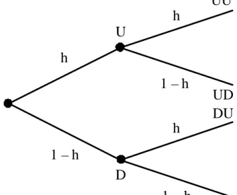
I do not presume a cut and dried distinction between natural buyers and the public. I imagine a continuum of agents uniformly arrayed between 0 and 1. Agent h on that continuum thinks the probability of good news (Up) is γUh = h, and the probability of bad news (Down) isγh
D= 1−h. The higher theh, the more optimistic
the agent.
The more optimistic an agent, the more natural a buyer he is. By having a continuum I avoid a rigid categorization of agents. The agents will choose whether to be borrowers and buyers of risky assets, or lenders and sellers of risky assets. There will be some break pointbsuch that those more optimistic withh > bare on one side of the market and and those less optimistic, with h < b, are on the other side. But this break pointb will be endogenous. See Diagram 1.
Natural buyers
public
Natural Buyers-Margins Theory of Crashes
h=0 h=1
2
Borrowing and Asset Pricing
Consider a simple example with one consumption good C, one asset Y, two time periods0,1, and two states of natureU andDin the last period. Suppose that each unit of Y pays either 1 or .2 of the consumption good, in the two states U or D, respectively. Imagine the asset as a mortgage that either pays in full or defaults with recovery .2. (All mortgages will either default together or pay off together). But it could also be an oil well that might be a gusher or small. Or a house with good or bad resale value next period. Let every agent own one unit of the asset at time 0 and also one unit of the consumption good at time 0. For simplicity we think of the consumption good as something that can be used up immediately as consumption c, or costlessly warehoused (stored) in a quantity denoted by w. Think of oil or cigarettes or canned food or simply gold (that can be used asfillings) or money. The agents h ∈ H only care about the total expected consumption they get, no matter when they get it. They are not impatient. The difference between the agents is only in the probabilitiesγh
U, γDh = 1−γUh each attaches to a good outcome vs bad.
To start with, let us imagine the agents arranged uniformly on a continuum, with agenth∈H = [0,1] assigning probability γUh =h to the good outcome.
See diagram 2.
More formally, denoting the amount of consumption ofC in states bycs, and the
Let each agent h ∈H⊂[0,1]
assign probability hto s= U
and probability 1 −hto s = D.
Agents with hnear 1are
optimists, agents with hnear 0
are pessimists.
Endogenous Collateral with Heterogeneous
Beliefs: A Simple Example
Suppose that 1unit of Ygives $1unit in state Uand .2units inD.
U D Y=.2 0 h 1 – h Figure 2 Y=1 0 by w0 we have uh(c0, y0, w0, cU, cD) =c0+γUhcU+γDhcD =c0+hcU + (1−h)cD eh = (ehCo, ehYo, eChU, ehCD) = (1,1,0,0)
Storing goods and holding assets provide no direct utility, they just increase income in the future.
Suppose the price of the asset per unit at time 0 is p, somewhere between 0 and 1. The agents h who believe that
h1 + (1−h).2> p
will want to buy the asset, since by paying p now they get something with expected payoff next period greater thanp and they are not impatient. Those who think
h1 + (1−h).2< p
will want to sell their share of the asset. I suppose there is no short selling, but I will allow for borrowing. In the real world it is impossible to short sell many assets other than stocks. Even when it is possible, only a few agents know how, and those typically are the optimistic agents who are most likely to want to buy. So the assumption of no short selling is quite realistic. But we shall reconsider this point shortly.
If borrowing were not allowed, then the asset would have to be held by a large part of the population. The price of the asset would be .677 or about .68. Agent h=.60values the asset at .68 =.60(1) +.40(.2). So all thoseh below.60will sell all they have, or .60(1) =.60 in aggregate. Every agent above .60 will buy as much as he can afford. Each of these agents has just enough wealth to buy1/.68≈ 1.5 more units, hence .40(1.5) = .60 units in aggregate. Since the market for assets clears at time 0, this is the equilibrium with no borrowing.
More formally, taking the price of the consumption good in each period to be 1 and the price of Y to be p, we can write the budget set without borrowing for each agent as
BNh(p) ={(c0, y0, w0, c1, c2)∈R5+ :c0+w0+p(y0 −1) = 1 cU =w0 +y0
cD=w0 + (.2)y0}.
Given the price p, each agent chooses the consumption plan (ch
0, y0h, w0h, ch1, ch2) in BNh(p) that maximizes his utility uh defined above. In equilibrium all markets must
clear Z 1 0 (ch0 +w0h)dh= 1 Z 1 0 y0hdh= 1 Z 1 0 chUdh= 1 + Z 1 0 wh0dh Z 1 0 chDdh=.2 + Z 1 0 w0hdh
In this equilibrium agents are indifferent to storing or consuming right away, so we can describe equilibrium as if everyone warehoused and postponed consumption by taking
p=.68
(ch0, y0h, w0h, ch1, ch2) = (0,2.5,0,2.5, .5)for h≥.60 (ch0, y0h, w0h, chU, chD) = (0,0,1.68,1.68,1.68) forh < .60.
When loan markets are created, a smaller group of less than 40% of the agents will be able to buy and hold the entire stock of the asset. If borrowing were unlimited, at an interest rate of 0, the single agent at the top would borrow so much that he would buy up all the assets by himself. And then the price of the asset would be 1, since at any price p lower than 1 the agents h just below 1 would snatch the asset away from h= 1. But this agent would default, and so the interest rate would not be zero, and the equilibrium allocation needs to be more delicately calculated.
2.1
Incomplete Markets
We shall restrict attention to loans that are non-contingent, that is that involve promises of the same amount ϕ in both states. It is evident that the equilibrium allocation under this restriction will in general not be Pareto efficient. For example, in the no borrowing equilibrium, everyone would gain from the transfer ofε >0units of consumption in state U from each h < .60 to each agent with h > .60, and the transfer of3ε/2units of consumption in state D from eachh > .60to each agent with h < .60. The reason this has not been done in the equilibrium is that there is no asset that can be traded that moves money from U to D or vice versa. We say that the asset markets are incomplete. We shall assume this incompleteness for a long time, until we consider Credit Default Swaps.
2.2
Collateral
We have not yet determined how much people can borrow or lend. In conventional economics they can do as much of either as they like, at the going interest rate. But in real life lenders worry about default. Suppose we imagine that the only way to enforce deliveries is through collateral. A borrower can use the asset itself as collateral, so that if he defaults the collateral can be seized. Of course a lender realizes that if the promise is ϕin both states, then with no-recourse collateral he will only receive
min(ϕ,1)if good news min(ϕ, .2)if bad news
The introduction of collateralized loan markets introduces two more parameters: how much can be promisedϕ, and at what interest rate r?
Suppose that borrowing were arbitrarily limited toϕ≤.2y0, that is suppose agents were allowed to promise at most .2 units of consumption per unit of the collateral Y they put up. That is a natural limit, since it is the biggest promise that is sure to be covered by the collateral. It also greatly simplifies our notation, because then there would be no need to worry about default. The previous equilibrium without borrowing could be reinterpreted as a situation of extraordinarily tight leverage, where we have the constraint ϕ≤0y0.
Leveraging, that is, using collateral to borrow, gives the most optimistic agents a chance to spend more. And this will push up the price of the asset. But since they can borrow strictly less than the value of the collateral, optimistic spending will still be limited. Each time an agent buys a house, he has to put some of his own money down in addition to the loan amount he can obtain from the collateral just purchased. He will eventually run out of capital.
We can describe the budget set formally with our extra variables. B.h2(p, r) ={(c0, y0, ϕ0, w0, c1, c2)∈R6+: c0+w0+p(y0−1) = 1 + 1 1 +rϕ0 ϕ0 ≤.2y0 cU =w0+y0−ϕ0 cD=w0+ (.2)y0−ϕ0}.
We use the subscript.2on the budget set to remind ourselves that we have arbitrarily fixed the maximum promise that can be made on a unit of collateral. At this point we could imagine that was a parameter set by government regulators.
Note that in the definition of the budget set, ϕ0 > 0 means that the agent is making promises in order to borrow money to spend more at time 0. Similarly, ϕ0 < 0 means the agent is buying promises which will reduce his expenditures on consumption and assets in period 0, but enable him to consume more in the future states U and D. Equilibrium is defined by the price and interest rate(p, r)and agent choices(ch
0, y0h, ϕh0, wh0, chU, cDh)inB.h2(p, r)that maximizes his utilityuh defined above. In equilibrium all markets must clear
Z 1 0 (ch0 +w0h)dh= 1 Z 1 0 y0hdh= 1 Z 1 0 ϕh0dh= 0 Z 1 0 chUdh= 1 + Z 1 0 wh0dh Z 1 0 chDdh=.2 + Z 1 0 w0hdh
Clearly the no borrowing equilibrium is a special case of the collateral equilibrium, once the limit .2 on promises is replaced by 0.
One can calculate that the equilibrium price of the asset is now.75. At that price agenth=.69is just indifferent to buying. Those h < .69 will sell all they have, and those h > .69 will buy all they can with their cash and with the money they can borrow. One can check that the top 31% of agents will indeed demand exactly what the bottom69% are selling.
Who would be doing the borrowing and lending? The top 31% is borrowing to the max, in order to get their hands on what they believe are cheap assetss. The bottom 69% do not need the money for buying the asset, so they are willing to lend it. And what interest rate would they get? 0% interest, because they are not lending
all they have in cash. (They are lending.2/.69 =.29<1per person). Since they are not impatient and they have plenty of cash left, they are indifferent to lending at 0%. Competition among these lenders will drive the interest rate to 0%.
More formally, letting the marginal buyer be denoted byh=b, we can define the equilibrium equations as
p=γUb1 + (1−γUb)(.2) = b1 + (1−b)(.2) p= (1−b)(1) +.2
b
The first equation says that the marginal buyer b is indifferent to buying the asset. The second equation says that the price of Y is equal to the amount of money the agents above b spend buying it, divided by the amount of the asset sold. The numerator is then all the top group’s consumption endowment, (1−b)(1), plus all they can borrow after they get their hands on all of Y, namely (1)(.2)/(1 +r) =.2. The denominator is comprised of all the sales of one unit of Y each by the agents below b.
We must also take into account buying on margin. An agent who buys the asset while simultaneously selling as many promises as he can will only have to pay down p−.2. His return will be nothing in the down state, because then he will have to turn over all the collateral to pay back his loan. But in the up state he will make a profit of 1−.2. Any agent like bwho is indifferent to borrowing or lending and also indifferent to buying or selling the asset, will be indifferent to buying the asset with leverage because
p−.2 =γUb(1−.2) =b(1−.2)
Clearly this equation is automatically satisfied as long as p is set to satisfy the first equation above; simply subtract .2 from both sides. Agents h > b will strictly prefer to buy the asset, and strictly prefer to buy the asset with as much leverag as possible (since they are risk neutral).
As we said, the large supply of durable consumption good, no impatience, and no default implies that the equilibrium interest rate must be 0. Solving the two equations above and plugging these into the agent optimization gives equilibrium
b=.69 (p, r) = (.75,0),
(ch0, y0h, ϕ0h, w0h, ch1, ch2) = (0,3.2, .64,0,2.6,0) for h≥.69 (ch0, y0h, ϕh0, w0h, ch1, ch2) = (0,0,−.3,1.45,1.75,1.75) for h < .69.
Compared to the previous equilibrium with no leverage, the price rises modestly, from .68 to .75, because there is a modest amount of borrowing. Notice also that even at the higher price, fewer agents hold all the assets (because they can afford to buy on borrowed money).
The lesson here is that the looser the collateral requirement, the higher will be the prices of assets. Had we defined another equilibrium by arbitrarily specifying the collateral limit of ϕ ≤ .1y0, we would have found an equilibrium price intermediate between .68 and .75. This has not been properly understood by economists. The conventional view is that the lower is the interest rate, then the higher will asset prices be, because their cashflows will be discounted less. But in the example I just described, where agents are patient, the interest rate will be zero regardless of the collateral restrictions (up to .2). The fundamentals do not change, but because of a change in lending standards, asset prices rise. Clearly there is something wrong with conventional asset pricing formulas. The problem is that to compute fundamental value, one has to use probablities. But whose probabilities?
The recent run up in asset prices has been attributed to irrational exuberance because conventional pricing formulas based on fundamental values failed to explain it. But the explanation I propose is that collateral requirements got looser and looser. We shall return to this momentarily, after we endogenize the collateral limits.
Before turning to the next section, let us be more precise about our numerical measure of leverage
leverage = .75
(.75−.2) = 1.4.
The loan to value is .2/.75 = 27%, the margin or haircut is.55/.75 = 73%. In the no borrowing equilibrium, leverage was obviously 1.
But leverage cannot yet be said to be endogenous, since we have exogenouslyfixed the maximal promise at .2. Why wouldn’t the most optimistic buyers be willing to borrow more, defaulting in the bad state of course, but compensating the lenders by paying a higher interest rate? Or equivalently, why should leverage be so low?
2.3
Equilibrium Leverage
Before 1997 there had been virtually no work on equilibrium margins. Collateral was discussed almost exclusively in models without uncertainty. Even now the few writers who try to make collateral endogenous do so by taking an ad hoc measure of risk, like volatility or value at risk, and assume that the margin is some arbitrary function of the riskiness of the repayment.
It is not surprising that economists have had trouble modeling equilibrium haircuts or leverage. We have been taught that the only equilibrating variables are prices. It seems impossible that the demand equals supply equation for loans could determine two variables.
The key is to think of many loans, not one loan. Irving Fisher and then Ken Arrow taught us to index commodities by their location, or their time period, or by the state of nature, so that the same quality apple in different places or different periods might have different prices. So we must index each promise by its collateral. A promise of .2 backed by a house is different from a promise of .2 backed by 2/3 of
a house. The former will deliver .2 in both states, but the latter will deliver .2 in the good state and only 1.33 in the bad state. The collateral matters.
Conceptually we must replace the notion of contracts as promises with the notion of contracts as ordered pairs of promises and collateral. Each ordered pair-contract will trade in a separate market, with its own price.
Contractj = (Promisej, Collateralj) = (Aj, Cj)
The ordered pairs are homogeneous of degree one. A promise of .2 backed by 2/3 of a house is simply 2/3 of a promise of .3 backed by a full house. So without loss of generality, we can always normalize the collateral. In our example we shall focus on contracts in which the collateral Cj is simply one unit of Y.
So let us denote by j the promise of j in both states in the future, backed by the collateral of one unit of Y. We take an arbitrarily large set J of such assets, but include j=.2.
The j = .2 promise will deliver .2 in both states, the j = .3 promise will deliver .3 after good news, but only .2 after bad news, because it will default there. The promises would sell for different prices, and different prices per unit promised.
Our definition of equilibrium must now incorporate these new promisesj ∈J and pricesπj.When the collateral is so big that there is no default, πj =j/(1 +r),where
ris the riskless rate of interest. But when there is default, the price cannot be derived from the riskless interest rate alone. Given the price πj, and given that the promises
are all non-contingent, we can always compute the implied nominal interest rate as 1 +rj =j/πj.
We must distinguish between sales ϕj > 0 of these promises (that is borrowing)
from purchases of these promises ϕj <0. The two differ more than in their sign. A
sale of a promise obliges the seller to put up the collateral, whereas the buyer of the promise does not bear that burden. The marginal utility of buying a promise will often be much less than the marginal disutillity of selling the same promise, at least if the agent does not otherwise want to hold the collateral.
We can describe the budget set formally with our extra variables. Bh(p, π) ={(c0, y0,(ϕj)j∈J, w0, c1, c2)∈R2+×R J ×R3+ : c0+w0+p(y0−1) = 1 + J X j=1 ϕjπj J X j=1 max(ϕj,0)≤y0 cU =w0+y0− J X j=1 ϕjmin(1, j) cD =w0+ (.2)y0− J X j=1 ϕjmin(.2, j)}.
Observe that in thefinal two equations we see that we are describing no-recourse col-lateral. Every agent delivers the same, namely the promise or the collateral, whichever is worth less. The loan market is thus completely anonymous; there is no role for asymmetric information about the agents because every agent delivers the same way. Lenders need only worry about the collateral, not about the identity of the borrowers. Observe thatϕj can be positive (making a promise) or negative (buying a promise),
and that either way the deliveries or receipts are given by the same formula.
The middle inequality describes the crucial collateral or leverage constraint. Each promise must be backed by collateral, and so the sum of the collateral requirements across all the promises must be met by the Y on hand.
Equilibrium is defined exactly as before, except that now we must have market clearing for all the contractsj ∈J.
Z 1 0 (ch0 +w0h)dh= 1 Z 1 0 y0hdh= 1 Z 1 0 ϕhjdh= 0, ∀j ∈J Z 1 0 chUdh= 1 + Z 1 0 wh0dh Z 1 0 chDdh=.2 + Z 1 0 w0hdh
It turns out that the equilibrium is exactly as before. The only asset that is traded is ((.2, .2),1), namely j = .2. All the other contracts are priced, but in equilibrium neither bought nor sold. Their prices can be computed by the value the marginal
buyerb=.69attributes to them. So the priceπ.3 of the.3promise is.27, much more than the price of the.2promise but less per dollar promised. Similarly the price of a promise of.4 is given below
π.2 =.69(.2) +.31(.2) = .2 1 +r.2 =.2/.2 = 1.00 π.3 =.69(.3) +.31(.2) = .269 1 +r.3 =.3/.269 = 1.12 π.4 =.69(.4) +.31(.2) = .337 1 +r.3 =.4/.337 = 1.19
Thus an agent who wants to borrow .2 using one house as collateral can do so at 0% interest. An agent who wants to borrow .269 with the same collateral can do so by promising 12% interest. An agent who wants to borrow .337 can do so by promising 19% interest. The puzzle of one equation determining both a collateral rate and an interest rate is resolved; each collateral rate corresponds to a different interest rate. It is quite sensible that less secure loans with higher defaults will require higher rates of interest.
What then do we make of my claim about "the" equilibrium margin? The surprise is that in this kind of example, with only one dimension of risk and one dimension of disagreement, only one margin will be traded! Everybody will voluntarily trade only the .2 loan, even though they could all borrow or lend different amounts at any other rate.
How can this be? Mr h = 1 thinks for every .75 he pays on the asset, he can get 1 for sure. Wouldn’t he love to be able to borrow more, even at a slightly higher interest rate? The answer is no! In order to borrow more, he has to substitute say a .4 loan for a .2 loan. He pays the same amount in the bad state, but pays more in the good state, in exchange for getting more at the beginning. But that is not rational for him. He is the one convinced the good state will occur, so he definitely does not want to pay more just where he values money the most.3
The lenders are people with h < .69 who do not want to buy the asset. They are lending instead of buying the asset because they think there is a substantial chance of bad news. It should be no surprise that they do not want to make risky loans, even if they can get a 19% rate instead of a 0% rate, because the risk of default is too high for them. Indeed the risky loan is perfectly correlated with the asset which they have already shown they do not want. Why should they give up more money 3More precisely, buying Y while simultaneously using it as collateral to sell any non-contingent
promise of at least .2 is tantamount to buying up Arrow securities at a price of b per unit of net payoffin state U. So h>b is indifferent to trading on any of the loan markets promising at least .2. By promising .4 per unit of Y instead of .2 he simply is buying fewer of the up Arrow securities per contract (because he must deliver more in the up state), but he can buy more contracts (since he is receiving more money at date 0). He can accomplish exactly the same thing selling less .2 promises.
at time 0 to get more money in a state U they do not think will occur? If anything, these pessimists would now prefer to take the loan rather than to give it. But they cannot take the loan, because that would force them to hold the collateral to back their promises, which they do not want to do.4
Thus the only loans that get traded in equilibrium involve margins just tight enough to rule out default. That depends of course on the special assumption of only two outcomes. But often the outcomes lenders have in mind are just two. And typically they do set haircuts in a way that makes defaults very unlikely. Recall that in the 1994 and 1998 leverage crises, not a single lender lost money on repo trades. Of course in more general models, one would imagine more than one margin and more than one interest rate emerging in equilibrium.
To summarize, in the usual theory a supply equals demand equation determines the interest rate on loans. In my theory equilibrium often determines the equilibrium leverage (or margin) as well. It seems surprising that one equation could determine two variables, and to the best of my knowledge I was thefirst to make the observation (in 1997 and again in 2003) that leverage could be uniquely determined in equilibrium. I showed that the right way to think about the problem of endogenous collateral is to consider a different market for each loan depending on the amount of collateral put up, and thus a different interest rate for each level of collateral. A loan with a lot of collateral will clear in equilibrium at a low interest rate, and a loan with little collateral will clear at a high interest rate. A loan market is thus determined by a pair (promise,collateral), and each pair has its own market clearing price. The question of a unique collateral level for a loan reduces to the less paradoxical sounding, but still surprising, assertion that in equilibrium everybody will choose to trade in the same collateral level for each kind of promise. I proved that this must be the case when there are only two successor states to each state in the tree of uncertainty, with risk neutral agents differing in their beliefs, but with a common discount rate. More generally I conjecture that the number of collateral rates traded endogenously will not be unique, but it will robustly be much less than the dimension of the state space, or the dimension of agent types.
2.3.1 Upshot of equilibrium leverage
We have shown that in the simple two state context, equilibrium leverage transforms the purchase of the collateral into the buying of the up Arrow security: the buyer of the collateral will simultaneously sell the promise of the entire down payoff of the collateral, so on net he is just buying the up Arrow security.
4More precisely, agents with h<b will want to trade their wealth for as much consumption as
they can get in the down state. But on account of the incompleteness of markets, no combination of buying, selling, borrowing on margin and so on can get them more in the down state than in the up state. So they strictly prefer making the .2 loan to lending, or borrowing with collateral, any loan promising more than .2 per unit of Y.
2.3.2 Endogenous leverage: reinforcer or dampener?
One can imagine many shocks to the economy that affect asset prices. These shocks will also typically change equilibrium leverage. Will the change in equilibrium leverage multiply the effect on asset prices, or dampen the effect? For most shocks, endogenous leverage will act as a dampener.
For example, suppose that agents become more optimistic, so that we now have γDh = (1−h)2 <1−h
γUh = 1−(1−h)
2 > h
for allh∈(0,1).Substituting these new values for the beliefs into the utility function, we can recompute equilibrium, and wefind that the price of Y rises to .89. But the equilibrium promise remains .2, and the equilibrium interest rate remains 0. Hence leverage falls to1.29 =.89/(.89−.2). The marginal buyer b=.63 is lower than before. In short, the positive news has been dampened by the tightening of leverage.
A similar situation prevails if agents see an increase in their endowment of the consumption good. The extra wealth induces them to demand more Y, the price of Y rises, but not as far as it would otherwise, because equilibrium leverage goes down. The only shock that is reinforced by the endogenous movement in leverage is a shock to the tail of the distribution of Y payoffs. If the tail payoff.2 is increased to .3, that will have a positive effect on the expected payoffof Y, but the effect on the price of Y will be reinforced by the expansion of equilibrium leverage. Negative tail events will also be multiplied, as we shall see later.
2.4
Fundamental Asset Pricing? Failure of Law of One Price
We have already seen enough to realize that assets are not priced by fundamentals in collateral equilibrium. We can make this more concrete by supposing, as in my 2003 paper, that we have two identical assets, blue Y and red Y, where blue Y can be used as collateral but red Y cannot. Suppose that every agent begins withβ units of blue Y and (1−β)units of red Y, in addition to one unit of the consumption good. Will the law of one price hold in equilibrium?
Will the two assets, which are perfect substitutes, both delivering 1 or .2 in the two states U and D, sell for the same price? Why would anyone pay more to get the same thing? The answer is that the collateralizable assets will indeed sell for a significant premium, even though no agent will pay more for the same thing. The most optimistic buyers will exclusively buy the blue asset by leveraging, and the mildly optimistic middle group will exclusively buy the red asset without leverage. The rest of the population will sell their assets and lend to the biggest optimists.
Will the scarcity of collateral tend to boost the blue asset prices above the asset prices we saw in the last section? What effect does the presence of leverage for the blue assets have on the red asset prices?
2.5
Legacy Assets vs New Assets
These questions bear on an important policy choice that is being made at the writing of this paper. As a result of the leverage crunch of 2007-2009, asset prices plummeted. One critical effect was that it became very difficult to support asset prices for new ventures that would allow for new activity. Who would buy a new mortgage (or new credit card loan, or new car loan) at 100 when virtually the same old asset could be purchased on the secondary market at 65?
Suppose the government wants to prop up the price of new assets, by providing leverage beyond what the market will provide. Given a fixed upper bound in (ex-pected) defaults, would the government do better to provide lots of leverage on just the new assets, or by providing moderate leverage on all the assets, new and legacy? At the time of this writing, the government appears to have adopted the strategy of leveraging only the new assets. Yet all the asset prices are rising.
I considered these very questions in my 2003 paper, anticipating the current de-bate, by examining the effect on asset prices of adjusting the fractionβ of blue assets. If the new assets represent say ν = 5% of the total, then taking β =ν = 5% corre-sponds to a policy of leveraging just the new assets. Taking β = 100% corresponds to leveraging the legacy assets as well.
To keep the notation simple, let us assume that using a blue asset as collateral, one can sell a promise j of .2, but that the red asset cannot serve as collateral for any promises.
The definition of equilibrium now consists of(r, pB, pR,(ch0, yh0B, y0hR, ϕh0, wh0, ch1, ch2)h∈H)
such that the individual choices are optimal in the budget sets
B.h2,B(p, r) ={(c0, y0B, y0R, ϕ0, w0, c1, c2)∈R7+ : c0+w0+pB(y0B−β) +pR(y0R−(1−β)) = 1 + 1 1 +rϕ0 ϕ0 ≤.2y0B cU =w0+y0B+y0R−ϕ0 cD =w0+ (.2)(y0B+y0R)−ϕ0}.
and markets clear Z 1 0 (ch0 +w0h)dh= 1 Z 1 0 y0hBdh=β Z 1 0 y0hRdh= 1−β Z 1 0 ϕh0dh= 0 Z 1 0 chUdh= 1 + Z 1 0 wh0dh Z 1 0 chDdh=.2 + Z 1 0 w0hdh
A moment’s thought will reveal that there will be an agent a indifferent between buying blue assets with leverage at a high price, and red assets without leverage at a low price. Similarly there will be an agent b < a who will be indifferent between buying red assets and selling all his assets. The optimistic agents with h > a will exclusively buy blue assets, the agents withb < h < awill exclisively hold red assets, and the agents withh < b will hold no assets and lend.
The equilibrium equations become
pR =b1 + (1−b)(.2) pR = (a−b) +pBβ(a−b) (1−β)(1−(a−b)) a(1−.2) pB−.2 = a1 + (1−a).2 pR pB = (1−a) +pR(1−β)(1−a) +.2β βa
Thefirst equation says that agentbis indifferent between buying red or not buying at all. The second equation says that the agents betweena andbcan just afford to buy all of the red Y that is being sold by the other(1−(a−b))agents, noting that their expenditure consists of the one unit of the consumption good and the revenue they get from selling offtheir blue Y. The third equation says thatais indifferent between buying blue with leverage, and red without. The last equation says that the top1−a agents can just afford to buy all the blue assets, by spending their endowment of the consumption good plus the revenue from selling their red Y plus the amount they can borrow using the blue Y as collateral.
fraction blue 1 0.5 0.05
a 0.6861407 0.841775 0.983891
b 0.6861407 0.636558 0.600066
pred 0.7489125 0.709246 0.680053
pblue 0.7489125 0.74684 0.742279
Suppose we begin with the situation more or less prevailing six months ago, with β = 0% and no leverage, just as in our veryfirst example where we found the assets priced at .677. By settingβ = 5% and thereby leveraging the 5% new assets (that is turning them into blue assets) the government can raise their price from .677 to .74. Interestingly this also raises the price of the red assets which remain without leverage, from .677 to .680. Providing the same leverage for more assets, by extendingβ to .5 or 1 and thereby leveraging some of the legacy assets, raises the value of all the assets! Thus if one wanted to raise the price of just the 5% new assets, the government should leverage all the assets, new and legacy. By holding promises down to .2, there would be no defaults.
This analysis holds some lessons for the current discussion about TALF, the gov-ernment program designed to inject leverage into the economy in 2009. The introduc-tion of leverage for new assets did raise the price of new assets substantially. It also raised the price of old assets that were not leveraged (although part of that might be due to the exectation that the government lending facilty will be extended to old assets as well). One might think that the best way to raise new asset prices is to give them scarcity value as the only leveraged assets in town. But on the contrary, the analysis shows that the price of the new assets could be boosted further by extending leverage to all the legacy assets, without increasing the amount of default.
The reason for this paradoxical conclusion is that optimistic buyers always have the option of buying the legacy assets at low prices. There must be substantial leverage in the new assets to coax them into buying if the new asset prices are much higher. By leveraging the legacy assets as well and thus raising the price of those assets, the government can undercut the returns from the alternative and increase demand for the new assets.
This analysis also has implications for spillovers from shocks across markets, a subject we return to later. The loss of leverage in one asset class can depress prices in another asset class whose leverage remains the same.
2.6
Complete Markets
Suppose there were complete markets. The distinctions between red and blue assets would be irrrelevant. The equilibrium would simply be ((pU, pD),(x0h, wh0, xhU, xhD))
assuming the price ofc0 is 1) and Z 1 0 (ch0 +w0h)dh= 1 Z 1 0 chUdh= 1 + Z 1 0 w0hdh Z 1 0 chDdh=.2 + Z 1 0 w0hdh (xh0, wh0, xhU, xhD)∈Bh(p) ={(x0, w0, xU, xD) : x0+w0+pUxU+pDxD ≤1 +pU1 +pD(.2)} (x0, w0, xU, xD)∈Bh(p)⇒uh(x0, xU, xD)≤uh(xh0, x h U, x h D)
It is easy to calculate that complete markets equilibrium occurs where(pU, pD) =
(.44, .56) and agents h > .44 spend all of their wealth of 1.55 buying 3.5 units of consumption each in state U and nothing else, giving total demand of(1−.44)3.5 = 2.0 and the bottom .44 agents spend all their wealth buying 2.78 units ofxD each, giving
total demand of.44(2.78) = 1.2in total.
The price of Y with complete markets is thereforepU1 +pD(.2) =.55, much lower
than the incomplete markets, leverage price of .75. Thus leverage can boost asset prices well above their "efficient" levels.
2.7
CDS and the Repo Market
The collateralized loan markets we have studied so far are similar to the Repo markets that have played an important role on Wall Street for decades. In these markets borrowers take their collateral to a dealer and use that to borrow money via non-contingent promises due one day later. The CDS is a much more recent contract.
The invention of the CDS or credit default swap moved the markets closer to complete. In our two state example with plenty of collateral, their introduction actually does lead to the complete markets solution, despite the need of collateral. In general, with more perishable goods, and goods in the future that are not tradable now, the introduction of CDS does not complete the markets.
A CDS is a promise to pay the principal default on a bond. Thus thinking of the asset as paying 1, or .2 if it defaults, the credit default swap would pay .8 in the down state, and nothing anywhere else. In other words, the CDS is tantamount to trading the down Arrow security.
The credit default swap needs to be collateralised. There are only two possible collaterals for it, the security, or the gold. A collateralisable contract promising an Arrow security is particularly simple, because it is obvious we need only consider versions in which the collateral exactly covers the promise. So choosing the nor-malizations in the most convenient way, there are essentially two CDS contracts to
consider, a CDS promising .2 in state D and nothing else, collateralized by the secu-rity, or a CDS promising 1 in state D, and nothing else, collateralized by a piece of the durable consumtion good gold. So we must add these two contracts to the Repo contracts we considered earlier.
It is a simple matter to show that the complete markets equilibrium can be im-plemented via the two CDS contracts. The agentsh > .44buy all the security Y and all the gold, and sell the maximal amount of CDS against all that collateral. Since all the goods are durable, this just works out.
2.7.1 The upshot of CDS
In this simple model, the CDS is the mirror image of the Repo. By purchasing an asset using the maximal leverage on the Repo market, the optimist is synthetically buying an up Arrow security (on net it pays a positive amount in the up state, and on net it pays nothing in the down state). The CDS is a down Arrow security. It is tantamount therefore, to letting the pessimists leverage. That is why the price of the asset goes down once the CDS is introduced.
Another interesting consequence is that the CDS kills the repo market. Buyers of the asset switch from selling repo contracts against the asset to selling CDS. It is true that since the introduction of CDS in late 2005 into the mortgage market, the repo contracts have steadily declined.
In the next section we ignore CDS and reexamine the repo contracts in a dynamic setting. Then we return to CDS.
3
The Leverage Cycle
If in the example bad news occurs and the value plummets to .2, there will be a crash. This is a crash in the fundamentals. There is nothing the government can do to avoid it. But the economy is far from the crash in period 0. It hasn’t happened yet. The marginal buyer thinks the chances of a fundamentals crash are only 31%. The average buyer thinks the fundamentals crash will occur with just 15% probability.
The point of the leverage cycle is that excess leverage followed by excessive delever-aging will cause a crash even before there has been a crash in the fundamentals, and even if there is no subsequent crash in the fundamentals. When the price crashes everybody will say it has fallen more than their view of the fundamentals warranted. The asset price is excessively high in the initial or over-leveraged normal economy, and after deleveraging, the price is even lower than it would have been at those tough margin levels had there never been the over-leveraging in the first place.
So consider the same example but with three periods instead of two. Suppose, as before, that each agent begins in states= 0 with one unit of money and one unit of the asset, and that both are perfectly durable. But now suppose the asset Y pays off after two periods instead of one period. After good news in either period, the asset
U
UU
UD
DU
DD
D
0
h
1 – h
1 – h
1 – h
h
h
1
1
1
.2
Crash
pays 1 at the end. Only with two pieces of bad news does the asset pay .2. The state space is nowS ={0, U, D, U U, U D, DU, DD}. We use the notation s∗ to denote the immediate predecessor ofs. Denote byγsh the probability h assigns to nature moving
from s∗ to s. For simplicity we assume that every investor regards the U vs D move from period 0 to period 1 as independent and identically distributed to the U vs D move of nature from period 1 to period 2, and more particularyγh
U =γDUh =h.
Diagram 3 here
This is the situation described in the introduction, in which two things must go wrong (i.e. two down moves) before there is a crash in fundamentals. Investors differ in their probability beliefs over the odds that either bad event happens. The move of nature from 0 to D lowers the expected payoffof the asset Y in every agent’s eyes, and also increases every agent’s view of the variance of the payoff of asset Y. The news creates more uncertainty, and more disagreement.
Suppose agents again have no impatience, but care only about their expected consumption of dollars. Formally, lettingcs be consumption in states,and letting ehs
be the initial endowment of the consumption good in state s, and letting yh
initial endowment of the asset Y before time begins, we have for all h∈[0,1] uh(c0, cU, cD, cU U, cU D, cDU, cDD) =c0+γUhcU+γDhcD+γUhγ h U UcU U +γhUγ h U DcU D +γDhγ h DUcDU +γDhγ h DDcDD =c0+hcU + (1−h)cD+h2cU U +h(1−h)cU D+ (1−h)hcDU + (1−h)2cDD (eh0, y0h∗, ehU, eDh, ehU U, ehU D, ehDU, ehDD) = (1,1,0,0,0,0,0,0)
We define the dividend of the asset by dU U = dU D = dDU = 1, and dDD = .2, and
d0 =dU =dD = 0.
The agents are now more optimistic than before, since agent h assigns only a probability of (1−h)2 to reaching the only state, DD, where the asset pays off .2. The marginal buyer from before,b=.69, for example, thinks the chances of DD are only (.31)2 =.09. Agent h =.87 thinks the chances of DD are only (.13)2 = 1.69%. But more importantly, if buyers can borrow short term, their loan at 0 will come due before the catastrophe can happen. It is thus much safer than a loan at D.
Assume that repo loans are one-period loans, so that loan sj promisesj in states sU and sD, and requires one unit of Y as collateral. The budget set can now be written iteratively, for each state s.
Bh(p, π) ={(cs, ys,(ϕsj)j∈J, ws)s∈S ∈(R2+×R J ×R+)1+S :∀s (cs+ws−ehs) +ps(ys−ys∗) =ys∗ds+ J X j=1 ϕsjπsj − J X j=1 ϕs∗jmin(ps+ds, j) J X j=1 max(ϕsj,0)≤ys}
In each state s the price of consumption is normalized to 1, and the price of the asset is ps and the price of loan sj promising j in states sU and sD is πsj. Agent
h spends if he consumes and stores more than his endowment or if he increases his holdings of the asset. His income is his dividends from last period’s holdings (by convention dividends in state s go the asset owner in s∗) plus his sales revenue from selling promises, less the payments he must make on previous loans he took out. Collateral is as always no recourse, so he can walk away from a loan payment if he is willing to give up his collateral instead. The agents who borrow (taking φsj >0)
must hold the required collateral.
The crucial question again is how much leverage will the market allow at each state s? By the logic we described in the previous section, it can be shown that in every state s, the only promise that will be actively traded is the one that makes the maximal promise on which there will be no default. Since there will be no default on this contract, it trades at the riskless rate of interest rs per dollar promised. Using
by redefining ϕs as the amount of the consumption good promised at state s for
delivery in the next period, in states sU and sD. The budget set then becomes Bh(p, r) ={(cs, ys, ϕs, ws)s∈S ∈R4(1++ S):∀s (cs+ws−ehs) +ps(ys−ys∗) =ys∗ds+ J X j=1 ϕs 1 1 +rs − ϕs∗ ϕs ≤ysmin(psU+dsU, psD +dsD)}
Equilibrium occurs at prices(p, r)such that when everyone optimizes in his budget set by choosing (ch
s, ysh, ϕhs, wsh)s∈S the markets clear in each state s
Z 1 0 (chs +whs)dh= Z 1 0 ehsdh+ds Z 1 0 ysh∗dh Z 1 0 yshdh= Z 1 0 yhs∗dh Z 1 0 ϕhsdh= 0
It will turn out in equilibrium that the interest rate is zero in every state. Thus at time 0, agents can borrow the minimum of the price of Y at U and at D, for every unit of Y they hold at 0. At U agents can borrow 1 unit of the consumption good, for every unit of Y they hold at U. At D they can borrow only .2 units of the consumption good, for every unit of Y they hold at D. In normal times, at 0, there is not very much bad that can happen in the short run. Lenders are therefore willing to lend much more on the same collateral, and leverage can be quite high. Solving the example gives the following prices. See Diagram 4.
The price of Y at time 0 of .95 occurs because the marginal buyer is h = .87. Assuming the price of Y is .69 at D and 1 at U, the most that can be promised at 0 using Y as collateral is .69. With an interest rate r0 = 0, that means .69 can be borrowed at 0 using Y as collateral. Hence the top 13% of buyers at time 0 can collectively borrow .69 (since they will own all the assets), and by adding their own .13 of money they can spend .82 on buying the .87 units that are sold by the bottom 87%. The price is.95≈.82/.87.
Why is there a crash from 0 to D? Well first there is bad news. But the bad news is not nearly as bad as the fall in prices. The marginal buyer of the asset at time 0, h =.87, thinks there is only a (.13)2 = 1.69% chance of ultimate default, and when he gets to D after the first piece of bad news he thinks there is a 13% chance for ultimate default. The news for him is bad, accounting for a drop in price of about 11 points, but it does not explain a fall in price from .95 to .69 of 26 points. In fact, no agent h thinks the loss in value is nearly as much as 26 points. The biggest optimist h= 1 thinks the value is 1 at 0 and still 1 at D. The biggest pessimist h = 0 thinks the value is .2 at 0 and still .2 at D. The biggest loss attributable to the bad news of
U
UU
UD
DU
DD
D
0
h
1 – h
1 – h
1 – h
h
h
1
1
1
R
Crash
.95
.69
1
arriving at D is felt by h=.5, who thought the value was .8 at 0 and thinks it is .6 at D. But that drop of .2 is still less than the drop of 26 points in equilibrium.
The second factor is that the leveraged buyers at time 0 all go bankrupt at D. They spent all their cash plus all they could borrow at time 0, and at time D their collateral is confiscated and used to pay off their debts: they owe .69 and their collateral is worth .69. Without the most optimistic buyers, the price is naturally lower.
Finally, and most importantly, the margins jump from (.95−.69)/.95 = 27% at U to (.69−.2)/.69 = 71% at D. In other words, leverage plummets from 3.6 = .95/(.95−.69) to 1.4 =.69/(.69−.2).
All three of these factors working together explain the fall in price.
leta be the marginal buyer in state 0.Then we must have pD=γDUb 1 +γDDb (.2)≡b1 + (1−b)(.2) pD= (1/a)(a−b) +.2 (1/a)b = 1.2a−b b a= b(1 +pD) 1.2 p0 = (1−a) +pD a a(1−pD) p0−pD ≡ γUa(1−pD) p0−pD =γUa1 +γDa γDUa γb DU ≡a1 + (1−a)a b a(1−pD) p0−pD ≡ γa U(1−pD) p0−pD = γa U1 +γDapD γa DU γb DU p0 ≡ a1 + (1−a)pDab p0
Thefirst equation says that the price at D is equal to the valuation of the marginal buyerbat D. Because he is also indifferent to borrowing, he will then also be indifferent to buying on the margin, a