Analysis and Actions on Graph Data
by Pin-Yu Chen
A dissertation submitted in partial fulfillment of the requirements for the degree of
Doctor of Philosophy
(Electrical and Computer Engineering) in The University of Michigan
2016
Doctoral Committee:
Professor Alfred O. Hero III, Chair Assistant Professor Danai Koutra Assistant Professor Daniel M. Romero
© Pin-Yu Chen 2016 All Rights Reserved
ACKNOWLEDGEMENTS
I am very fortunate to have Professor Alfred Hero as my advisor. During my doctoral study he has opened a new research door in graph data analytics for me, and has been continuously providing his full support, both in research and career development. I am also very fortunate to have Professor Vijay Subramanian, Professor Daniel Romero, and Professor Danai Koutra as my dissertation committee members. Their efforts and comments have made my dissertation more solid and profound.
I would like to thank members in the Hero group for their friendship and research discussion, especially to Sijia Liu for exciting research collaboration, to Yu-Hui Chen for providing his dissertation template, and to Michele Feldkamp in the EECS office for her administrative assistance. I also would like to thank Pai-Shun Ting and Chun-Chen Tu for their friendship and company in weekly grocery shopping. You have made Ann Arbor an even more unforgettable place. Outside of University of Michigan, I would like to thank Doctor Sutanay Choudhury at Pacific Northwest National Laboratory for giving me an internship opportunity, thank Siheng Chen at Carnegie Mellon University for his friendship and remarkable insight in graph signal processing, thank Professor Shin-Ming Cheng at National Taiwan University of Science and Technology for his friendship and productive research collaboration.
Lastly, I woule like to thank my parents, my brother Pin-Jung Chen, my girl friend Pin-Yu Chen, my best friends Chun-Yu Yang and Domi Liu, and other families and friends in Taiwan, for being part of my life. Your encouragement and company have fulfilled my life and have given me the momentum for becoming a better man.
TABLE OF CONTENTS
DEDICATION . . . ii
ACKNOWLEDGEMENTS . . . iii
LIST OF FIGURES . . . ix
LIST OF TABLES . . . xvii
LIST OF APPENDICES . . . xviii
ABSTRACT . . . xix
CHAPTER I. Introduction . . . 1
1.1 Motivation . . . 1
1.2 Highlights of the Dissertation . . . 2
1.3 Matrix Representations for Graphs . . . 2
1.3.1 Block model for graph data . . . 3
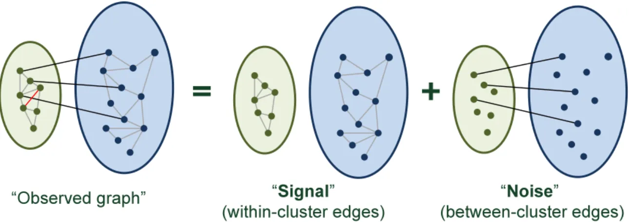
1.3.2 A signal plus noise perspective . . . 4
1.3.3 Graph Laplacian matrices and their properties . . . 5
1.3.4 Spectral clustering . . . 6
1.4 Overview of Graph Clustering Methods . . . 7
1.4.1 Graph clustering methods and analysis for single-layer graphs . . . 8
1.4.2 Model order selection . . . 9
1.4.3 Graph clustering methods and analysis for multilayer graphs . . . 10
1.5 Overview of Node Centrality Measures . . . 11
1.6 Dissertation Outline and Contributions . . . 13
1.7 List of Relevant Publications . . . 16
1.7.1 Journal publications . . . 16
1.7.2 Conference publications . . . 16
II. Incremental Method for Spectral Graph Clustering of
In-creasing Orders . . . 18
2.1 Incremental Eigenpair Computation for Graph Laplacian Ma-trices . . . 20
2.1.1 Notation for eigenpairs . . . 20
2.1.2 Theoretical foundations of the proposed method . . 20
2.1.3 Incremental eigenpair computation method . . . 22
2.1.4 Computational complexity analysis . . . 24
2.2 Experimental Results . . . 25
III. Phase Transitions in Spectral Modularity Method under a Stochastic Block Model . . . 27
3.1 Phase Transition Analysis . . . 28
3.2 Numerical Experiments . . . 35
3.2.1 Validation of phase transition analysis . . . 35
3.2.2 Empirical estimator of the phase transition threshold 37 IV. Phase Transitions in Spectral Graph Clustering under the Random Interconnection Model . . . 38
4.1 Random Interconnection Model (RIM) and Spectral Clustering 39 4.1.1 Random interconnection model (RIM) . . . 39
4.1.2 Mathematical formulation for spectral graph clustering 40 4.2 Breakdown Condition and Phase Transition Analysis . . . 41
4.3 Numerical Experiments: Validation of Phase Transitions in Simulated Networks . . . 50
V. AMOS: An Automated Model Order Selection Criterion for Spectral Graph Clustering. . . 52
5.1 Automated Model Order Selection (AMOS) Algorithm for Spec-tral Graph Clustering . . . 53
5.1.1 Input graph data and spectral clustering . . . 54
5.1.2 RIM test via p-value for local homogeneity testing . 54 5.1.3 Phase transition tests . . . 56
5.1.4 Computational complexity analysis . . . 59
5.2 Experiments: Automated model order selection (AMOS) on real-world network data . . . 60
5.2.1 External and internal clustering metrics . . . 63
VI. Multilayer Spectral Graph Clustering via Convex Layer Ag-gregation . . . 66
6.1 Multilayer Graph Model and Spectral Graph Clustering via
Convex Layer Aggregation . . . 68
6.1.1 Multilayer graph model . . . 68
6.1.2 Multilayer signal plus noise model . . . 70
6.1.3 Multilayer spectral graph clustering via convex layer aggregation . . . 71
6.2 Performance Analysis of Multilayer Spectral Graph Clustering via Convex Layer Aggregation . . . 72
6.2.1 Breakdown condition for multilayer SGC via convex layer aggregation . . . 74
6.2.2 Phase transitions in multilayer SGC under block-wise identical noise . . . 74
6.2.3 Phase transitions in multilayer SGC under block-wise non-identical noise . . . 78
6.3 MIMOSA: Multilayer Iterative Model Order Selection Algorithm 79 6.3.1 Input data . . . 80
6.3.2 Layer weight adaptation . . . 80
6.3.3 Block-wise homogeneity test . . . 82
6.3.4 Clustering reliability test under the block-wise iden-tical noise model . . . 82
6.3.5 Clustering reliability test under the block-wise non-identical noise model . . . 85
6.3.6 A signal-to-noise ratio criterion for final clustering results . . . 86
6.3.7 Computational complexity analysis . . . 87
6.4 Numerical Experiments . . . 88
6.4.1 Phase transitions in multilayer SGC via convex layer aggregation . . . 88
6.4.2 The effect of layer weight vector on multilayer SGC via convex layer aggregation . . . 89
6.5 MIMOSA on Real-World Multi-Layer Graphs . . . 92
6.5.1 Dataset descriptions . . . 92
6.5.2 Performance evaluation . . . 94
VII. Local Fiedler Vector Centrality and Deep Community Detec-tion . . . 99
7.1 Algebraic Connectivity and Fiedler Vector . . . 101
7.1.1 Algebraic connectivity . . . 101
7.1.2 Fiedler vector . . . 102
7.2 Deep Community Detection . . . 102
7.3 The Proposed Node and Edge Centrality: Local Fiedler Vector Centrality (LFVC) . . . 106
7.3.2 Node-LFVC . . . 108
7.3.3 Monotonic submodularity and greedy removals . . . 109
7.4 Deep Community Detection on Real-world Datasets . . . 112
7.4.1 Dolphin social network . . . 112
7.4.2 Zachary’s karate club . . . 113
7.4.3 Coauthorship among network scientists . . . 115
7.4.4 Last.fm online music system . . . 116
VIII. Identifying Influential Links for Event Propagation on Twit-ter: A Network of Networks Approach . . . 121
8.1 The NoN Structure of Event Propagation on Twitter . . . 123
8.2 Methodology . . . 124
8.2.1 Event propagation model . . . 124
8.2.2 Surrogate function for event propagation . . . 126
8.2.3 LES: left eigenvector score . . . 127
8.3 Experiments on Twitter Traces . . . 129
8.3.1 Experiment setup and dataset description . . . 129
8.3.2 Performance evaluation . . . 132
IX. Assessing and Safeguarding Network Resilience to Nodal At-tacks . . . 134
9.1 Resilience of Western US States Power Grid Topology to Cen-trality Attacks . . . 137
9.2 Preventive Approaches to Centrality Attacks . . . 139
9.2.1 Edge addition method . . . 139
9.2.2 Edge rewiring method . . . 140
9.3 Performance Evaluation . . . 142
X. Graph-Theoretic Action Recommendations for Cyber Resiliency144 10.1 Tripartite Network Model and Iterative Reachability Compu-tation of Lateral Movement . . . 148
10.1.1 Notations and tripartite graph model . . . 148
10.1.2 Reachability of lateral movement on user-host access graph . . . 149
10.1.3 Reachability of lateral movement on host-application graph . . . 151
10.1.4 Reachability of lateral movement on tripartite user-host-application graph . . . 153
10.2 Segmentation on User-Host Graph . . . 153
10.3 Hardening on Host-Application Graph . . . 158
10.4 Experimental Results . . . 162
10.4.2 Lateral movement and segmentation on user-host graph163 10.4.3 Lateral movement and hardening on host-application
graph . . . 164
10.4.4 Lateral movement, segmentation and hardening on tripartite graph . . . 165
10.5 Benchmark: Performance Evaluation on Actual Lateral Move-ment Attacks . . . 166
XI. Conclusion and Future Work . . . 170
11.1 Future work . . . 173
APPENDICES . . . 175
LIST OF FIGURES
Figure
1.1 An illustration of the connectivity structure of a graph generated from a block model with K = 2 clusters. . . 5 1.2 An illustration of graph spectral decomposition methods for graph
clustering. Graph spectral decomposition methods transform the ob-served graph into a representation in a low-dimensional vector space to reveal the ground-truth clusters. . . 7 2.1 Sequential eigenpair computation time on Erdos-Renyi random graphs
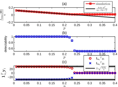
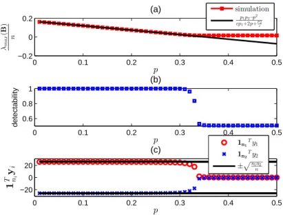
with edge connection probability p= 0.1. The markers are averaged computation time of 50 trials and the error bar represents standard deviation. . . 25 3.1 Validation of theoretical critical phase transition threshold (3.24)
for two communities generated by a stochastic block model. The curves represent averages over 100 realizations of the model. Here
n1 = n2 = 2000 and p1 = p2 = 0.25 so that the predicted critical
phase transition is p∗ = 0.25. (a) When p < p∗, λmax(B)
n converges to p1p2−p2
cp1+2p+pc2 as predicted in (3.18). Whenp > p
∗, λmax(B)
n converges to 0 as predicted by (3.23). (b) Fraction of nodes that are correctly identi-fied using the spectral modularity method. Community detectability undergoes a phase transition from perfect detectability to low de-tectability at p = p∗. (c) The spectral modularity method fails to detect the communities when p > p∗ since the components of the largest eigenvector of B, y1 and y2, undergo transitions at p=p∗ as
predicted by (3.19) and (3.22). . . 35 3.2 Validation of theoretical critical phase transition threshold (3.24) for
two communities generated by a stochastic block model. The curves represent averages over 100 realizations of the model. Heren1 = 1000,
n2 = 2000,p1 = 0.5, andp2 = 0.25 so that the predicted critical phase
transition is p∗ = 0.3536. Similar phase transition phenomenon can be observed for this network setting. . . 36
4.1 Phase transition of clusters generated by Erdos-Renyi random graphs.
K = 3,n1 =n2 =n3 = 8000, andp1 =p2 =p3 = 0.25. The empirical
critical phase transition threshold value predicted by Theorem 4.2 is
p∗ = 0.2301. . . 50 4.2 Phase transition of clusters generated by the Watts-Strogatz small
world network model. K = 3, n1 =n2 =n3 = 1000, average number
of neighbors = 200, and rewire probability for each cluster is 0.4, 0.4, and 0.6. The empirical critical threshold value predicted by Theorem 4.2 is p∗ = 0.0985. . . 51 4.3 Phase transition of clusters generated by Erdos-Renyi random graphs
with exponentially distributed edge weight with mean 10. K = 3,
n1 = n2 = n3 = 8000, and p1 = p2 = p3 = 0.25. The
pre-dicted phase transition threshold curve from Theorem 4.9 is p·W = Kmink∈{1,2,...,K}S2:K(Lk)
(K−1)n . . . 51 5.1 Flow diagram of the proposed automated model order selection (AMOS)
scheme in spectral graph cluster (SGC). . . 54 5.2 IEEE reliability test system [68]. Normalized (unnormalized) spectral
graph clustering (SGC) misidentifies 2 (3) nodes, whereas self-tuning spectral clustering fails to identify the third cluster. . . 61 5.3 The Hibernia Internet backbone map across Europe and North
Amer-ica [85]. Cities of different continents are perfectly clustered via au-tomated SGC, whereas one city in North America is clustered with the cities in Europe via self-tuning spectral clustering. Automated clusters found by AMOS, including city names, can be found in Fig. D.3. . . 61 5.4 The Cogent Internet backbone map across Europe and North
Amer-ica [85]. Clusters from automated SGC are consistent with the ge-ographic locations, whereas clusters from self-tuning spectral clus-tering are inconsistent with the geographic locations. Automated clusters found by AMOS, including city names, can be found in Fig. D.4. . . 62 5.5 Minnesota road map [64]. Clusters from automated SGC are aligned
with the geographic separations, whereas some clusters from self-tuning spectral clustering are inconsistent with the geographic sep-arations and self-tuning spectral clustering identifies several small clusters. . . 63 6.1 Flow diagram of the proposed multilayer iterative model order
selec-tion algorithm (MIMOSA) for multilayer spectral graph clustering (SGC). . . 81
6.2 Phase transitions in the accuracy of multilayer SGC with respect to different layer weight vector w = [w1 w2]T for the two-layer
corre-lated graph model. n1 = n2 = n3 = 1000, q11 = 0.3, q10 = 0.2,
q01 = 0.1, and q00= 0.4. The results are averaged over 10 runs. For
a given w, the variations in the noise level{p(`)}2
`=1 indeed separates
the accuracy of multilayer SGC into a reliable regime and an unreli-able regime. Furthermore, the critical value that separates these two regimes are successfully predicted by Theorem 6.2. . . 89 6.3 Phase transitions in the geometric mean of cluster detectability from
multilayer SGC via convex layer aggregation for the two-layer cor-related graph model, where w1 is uniformly sampled from the [0,1]
with unit interval 0.1. n1 = n2 = n3 = 500, q11 = 0.3, q10 = 0.2,
q01 = 0.1, and q00 = 0.4. The results are averaged over 10 runs.
It can be observed that the universal phase transition lower bound predicted by (6.4) indeed specifies a regime where any layer weight vector w ∈ W2 can lead to correct clustering results. Similarly for
the universal phase transition upper bound predicted by (6.5). . . . 90 6.4 The effect of the layer weight vectorw= [w1 w2]T on the accuracy of
multilayer SGC with respect to difference noise level{p(`)}2
`=1 for the
two-layer correlated graph model. n1 = n2 = n3 = 1000, q11 = 0.3,
q10 = 0.2, q01 = 0.1, and q00 = 0.4. The results are averaged over 50
runs. Fig. 6.4 (a) shows that in the case of low noise level for each layer, any layer weight vector w∈ W2 can lead to correct clustering
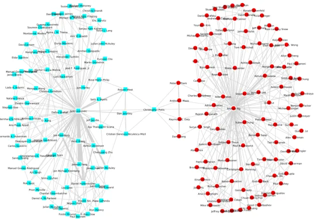
result. Fig. 6.4 (b) and (c) show that if one layer has high noise level, then there may exist a critical value w∗1 ∈ [0,1] that separates the cluster detectability into a reliable regime and an unreliable regime. Furthermore, the critical value w1∗ is shown to satisfy the equation in (6.15) derived from Theorem 6.2. Fig. 6.4 (d) shows that in the case of high noise level for each layer, no layer weight vector can lead to correct clustering result, and the cluster detectability is similar to random guessing of clustering accuracy 33.33%. . . 91 6.5 Ground-truth clusters of the collected Leskovec-Ng collaboration
net-work. Nodes represent researchers, edges represent the strength of coauthorship [141,177], and colors and shapes represent two clusters - “Leskovec’s collaborator” (cyan square) or “Ng’s collaborator” (red circle). . . 95 6.6 Illustration of ground-truth clusters and the clusters found by
MI-MOSA for the VC 7th grader social network dataset. Fig. 6.6 (a) displays the ground-truth clusters, where nodes 1 to 12 are boys (la-beled by blue color) and nodes 13 to 29 are girls (la(la-beled by red color). Fig. 6.6 (b) to (d) display the clusters (labeled by different colors) found by MIMOSA on each layer. Comparing to the ground-truth clusters, MIMOSA correctly group all nodes into 2 clusters except node 9, since node 9 has no edge connections in Fig. 6.6 (c) and (d), and has more connections to girls than boys in Fig. 6.6 (a). . . 98
7.1 An illustration of deep community detection. The entire network is a realization of the two-community stochastic block model withp2 =p.
That is, the first block is the deep community and the second block only contains spurious edges. The network size n = 50 and deep community sizen1 =ndeep = 20. The parameters cin=ndeep·p1 and
cout = n2 ·p. The nodes in the deep community are marked by red
solid circle, and the other nodes are marked by blue solid rectangles. The left and right columns represent adjacency matrices and their corresponding graphs, respectively. It is observed when cin is fixed,
the deep community is more difficult to be detected as cout increases. 103
7.2 Dolphin social network [96] with n = 62 nodes and m = 159 edges. (a) The modularity method. (b) Edge-LFVC community detection with h = 6 edge removals. (c) Node-LFVC community detection with q = 4 node removals. Using node-LFVC, we are able to iden-tify the four dolphins that interact with two groups as marked by nodes in gray circles. This algorithm, defined by Algorithm 7.1, de-tects that these four nodes are members of the two communities. The result of spectral clustering is shown in the supplementary file1. Spectral clustering results in the same discovered communities as the proposed edge-LFVC community detection method. However, unlike the proposed node-LFVC method it does not explicitly identify the four mixed membership dolphins that connect the two communities. 113 7.3 The modularity method on Zachary’s karate club [173] with n = 34
nodes and m= 78 edges. . . 114 7.4 Edge-LFVC community detection on Zachary’s karate club [173] with
n = 34 nodes and m = 78 edges. For g = 3 and 4, the only node with a single acquaintance is excluded from any deep community. . 115 7.5 Node-LFVC community detection on Zachary’s karate club [173] with
n = 34 nodes and m = 78 edges. Important communities and key members are discovered using node-LFVC. This also demonstrates how the singleton survivors (nodes with black X labels) interact through the deep communities. The result of spectral clustering is shown in the supplementary file1. When g = 4, spectral clustering
yields imbalanced communities (one community has single node). . . 116 7.6 Yamir Moreno’s local 2-hop coauthorship network (from part of the
network of coauthorship among network scientists [106] having n = 379 nodes and m = 914 edges). Moreno has 14 coauthors (marked by light orange color) and his coauthors have 35 coauthors. The modularity method [106] detects that Moreno is a member of only one large community (dashed box in gray). The proposed LFVC method detects Moreno as belonging to two separate communities indicated by red and blue nodes, respectively. . . 117
7.7 Mark Newman’s local 1-hop coauthor network in the network scien-tist coauthorship graph [106]. The proposed LFVC method detects Newman as belonging to 5 communities (marked by different ver-tex shapes and colors in solid boxes) and being associated with 3 singleton survivors (marked by black X label). Notably, Lusseau is detected as singleton survivor since his research area is primarily in zoology. As shown in gray dashed box, the modularity method [106] detects 25 out of 28 scholars as being in a single community, and the top left 3 scholars as belonging to 3 different communities. . . 118 7.8 Friendship in Last.fm online music system [21] with n = 1843 nodes
and m = 12668 edges. (a) Normalized largest community size de-creases in the number of node removals at different rates under dif-ferent node centralities. (b) Discovered communities with respect to node removals using different node centralities. Node-LFVC outper-forms other node centralities in terms of minimizing the largest com-munity size, and while being capable of detecting more communities in the network for the first 50 removals. . . 119 7.9 Residual sum of community similarity (RSCS) in Last.fm network.
The residual sum of community similarity based on node-LFVC out-performs other centralities, which indicates that node removals based on node-LFVC can best detect deep communities that share common interest in artists. . . 120 8.1 The three collected retweeter networks with user language identifying
the Network of Networks (NoN) structure. A retweeter is represented by a node with language setting denoted by its color/number. An edge between two nodes indicates that the event is retweeted from one node to another. The node 0 represents the virtual source of event propagation. For succinct representation, we grouped all the same-language leaf retweeters of a single node into a small node. It is observed that an event is first disseminated by some seed nodes, and other nodes tend to retweet the event from a same-language node.123 8.2 The effect of removing top-score follower links on the collected
Twit-ter datasets in Table 8.1. Event reachability is the fraction of users who can still post or retweet the event after some follower links are re-moved from the original Twitter follower network. It is observed that using the proposed LES and exploiting the NoN structure, the NoN-LES-Bet method can achieve remarkable reduction in event reacha-bility. The results suggest that LES indeed reflects the level of impor-tance of a follower link for event propagation, and between-network follower links are crucial to event propagation. . . 131
8.3 Fraction of between-network follower links in different link removal methods. Comparing to Fig. 8.2, although the fraction of removed between-network follower links of NoN-LES-Bet and NoN-NetMelt-Bet are similar, the follower links identified by NoN-LES-NoN-NetMelt-Bet are more influential in event propagation as their removals result in lower event reachability. . . 133 9.1 Resilience of network connectivity to different centrality attacks on
the power grid topology of western US states [163]. This network contains 4941 nodes and 6594 edges, where nodes represent power stations and edges represent power lines. By removing roughly 0.2% of the nodes in the network based on an LFVC attack, the largest component size is reduced to nearly half of its original size. . . 138 9.2 Network connectivity when restricted to 10 greedy node removals
on the power grid topology of western US states [163]. For the edge addition method, the network connectivity can be enhanced from 54% to 80% under LFVC attacks by adding one edge. The proposed edge rewiring method can perform as well as the edge addition method without introducing additional edges in the network. . . 142 9.3 Network connectivity when restricted to 20 greedy node removals on
the power grid topology of western US states [163]. For the edge addition method, 11 additional edges are required to enhance the network connectivity from 29% to 82%. The proposed edge rewiring method requires only 12 edge rewires to achieve the same performance as the edge addition method, which means that we only need to rewire fewer than 0.4% of edges to make it resilient to centrality attacks. . 143 10.1 An illustration of a cyber attack using privilege escalation techniques. 145 10.2 (a) Illustration of a tripartite network consisting of a set of users,
a set of hosts and a set of applications. (b) Segmentation in user-host access graph. The user Charlie modifies his access configuration by disabling the access of the existing account (Charlie-2) to host H3 and by creating a new user account (Charlie-1) for accessing H3 such that an attacker cannot reach the data server H5 though the printer H3 if Charlie-2 is compromised. (c) Edge hardening in host-application graph via additional firewall rules on all network flows to H5 through HTTP. (d) Node hardening in host-application graph via system update or security patch installation on H5. . . 146 10.3 The effect of segmentation on the user-host access graph. (a)
Reach-ability with respect to different segmentation strategies. (b) Fraction of newly created user accounts from segmentation. . . 164
10.4 The effect of known user-host access information on lateral movement attacks. (a) Greedy segmentation without score recalculation. (b) Greedy segmentation with score recalculation. (c) Greedy host first segmentation. (d) Greedy user first segmentation. Lateral movement attacks can be constrained in terms of reachability when sufficient segmentation is implemented and the user-host access information is limited to an attacker. . . 165 10.5 The effect of hardening on host-application graph. (a) Reachability
with respect to different edge hardening strategies. (b) Reachability with respect to different node hardening strategies. . . 166 10.6 The effect of segmentation and hardening on lateral movement attack
in user-host-application tripartite graph. (a) Greedy segmentation w/o score recalculation, greedy edge hardening w/o score recalcula-tion, and greedy node hardening with score ρ. (b) Greedy segmen-tation w/ score recalculation, greedy edge hardening w/ score recal-culation, and greedy node hardening with score ρ. (c) Greedy host first segmentation, greedy edge hardening w/o score recalculation, and greedy node hardening with score ρJ. (d) Greedy host first seg-mentation, greedy edge hardening w/ score recalculation, and greedy node hardening with scoreρJ. . . . 167 10.7 Performance evaluation on the collected benchmark dataset. Using
our proposed approaches, the lateral movement attacks can be further restrained by incorporating the heterogeneity of the cyber system. 168 B.1 The effect of community size on phase transition. The phase
transi-tion phenomenon hold for communities of small sizes, and the empiri-cal phase transition threshold gets closer to the predicted asymptotic threshold p∗ = 0.25 as the community size increases. . . 182 C.1 Phase transition of clusters generated by Erdos-Renyi random graphs.
K = 3, (n1, n2, n3) = (6000,8000,10000), and p1 = p2 = p3 = 0.25.
The empirical lower bound pLB = 0.1373 and the empirical upper
bound pUB= 0.2288. The results in (a) are averaged over 50 trials. . 195
C.2 Phase transition of clusters generated by the Watts-Strogatz small world network model. K = 3, (n1, n2, n3) = (1500,1000,1000),
av-erage number of neighbors = 200, and rewire probability for each cluster is 0.4, 0.4, and 0.6. The empirical lower and upper bounds are pLB = 0.0602 andpUB = 0.0902. The results in (a) are averaged
over 50 trials. . . 196 C.3 Sensitivity of cluster detectability to the inhomogeneous RIM. The
results are average over 50 trials and error bars represent standard deviation. (a) Clusters generated by Erdos-Renyi random graphs.
K = 3, n1 = n2 = n3 = 8000, p1 = p2 = p3 = 0.25, and p0 = 0.15.
(b) Clusters generated by the Watts-Strogatz small world network model. K = 3, n1 = n2 =n3 = 1000, average number of neighbors
= 200, and rewire probability for each cluster is 0.4, 0.4, 0.6, and
D.1 Clusters found with the nonbacktracking matrix method [87, 139]. For IEEE reliability test system, 8 nodes are clustered incorrectly. For Hibernia Internet backbone map, 3 cities in the north America are clustered with the cities in Europe. For Cogent Internet back-bone map, the clusters are inconsistent with the geographic locations. For Minnesota road map, some clusters are not aligned with the ge-ographic separations. . . 202 D.2 Clusters found with the Louvain method [18]. For IEEE reliability
test system, the number of clusters is different from the number of actual subgrids. For Hibernia and Cogent Internet backbone maps, although the clusters are consistent with the geographic locations, the Louvain method tends to identify clusters with small sizes. For Minnesota road map, the clusters are inconsistent with the geographic separations. . . 203 D.3 2 clusters found with the proposed automated model order selection
(AMOS) algorithm for the Hibernia Internet backbone map with city names. The clusters are consistent with the geographic locations in the sense that one cluster contains cities in America and the other cluster contains cities in Europe. . . 204 D.4 4 clusters found with the proposed automated model order selection
(AMOS) algorithm for the Cogent Internet backbone map with city names. Clusters are separated by geographic locations except for the cluster containing cities in North Eastern America and West Europe due to many transoceanic connections. . . 205
LIST OF TABLES
Table
1.1 Dissertation outline with respect to two actions on graphs . . . 13 2.1 Utility of the established lemmas, corollaries, and theorems in
Chap-ter II. . . 21 5.1 Summary of real-world single-layer graph datasets. . . 60 5.2 Summary of the number of identified clusters (K) and the external
and internal clustering metrics. “F” stands for F-measure and “C” stands for conductance. “NB” refers to the nonbacktracking matrix method, and “ST” refers to the self-tuning method. “-” means “not available” due to lack of ground-truth cluster labels. For each dataset, the method that leads the best clustering metric is highlighted in bold face. AMOS is shown to outperform most clustering methods for all datasets. . . 65 6.1 Summary of real-world multilayer graph datasets. . . 94 6.2 Summary of the number of identified clusters (K) and the external
and internal clustering metrics. “NA” means “not applicable”, and “-” means “not available” due to lack of ground-truth cluster labels. For each dataset, the method that leads the highest clustering metric is highlighted in bold face. . . 97 8.1 Statistics of the collected events and Twitter follower networks . . . 129 10.1 Utility of the proposed algorithms and established theoretical results
in Chapter X. . . 148 10.2 List of main notations and symbols in Chapter X. . . 149
LIST OF APPENDICES
Appendix
A. Appendix of Chapter II . . . 176
B. Appendix of Chapter III . . . 180
C. Appendix of Chapter IV . . . 183
D. Appendix of Chapter V . . . 198
E. Appendix of Chapter VI . . . 206
F. Appendix of Chapter VII . . . 217
G. Appendix of Chapter VIII . . . 222
ABSTRACT
Analysis and Actions on Graph Data by
Pin-Yu Chen
Chair: Alfred O. Hero III
Graphs are commonly used for representing relations between entities and handling data processing in various research fields, especially in social, cyber and physical networks. Many data mining and inference tasks can be interpreted as certain actions on the associated graphs, including graph spectral decompositions, and insertions and removals of nodes or edges. For instance, the task of graph clustering is to group similar nodes on a graph, and it can be solved by graph spectral decompositions. The task of cyber attack is to find effective node or edge removals that lead to maximal disruption in network connectivity.
In this dissertation, we focus on the following topics in graph data analytics: 1. Fundamental limits of spectral algorithms for graph clustering in single-layer
and multilayer graphs.
2. Efficient algorithms for actions on graphs, including graph spectral decomposi-tions and inserdecomposi-tions and removals of nodes or edges.
3. Applications to deep community detection, event propagation in online social networks, and topological network resilience for cyber security.
For 1, we established fundamental principles governing the performance of graph clustering for both spectral clustering and spectral modularity methods, which play an important role in unsupervised learning and data science. The framework is then extended to multilayer graphs entailing heterogeneous connectivity information.
For 2, we developed efficient algorithms for large-scale graph data analytics with theoretical guarantees, and proposed theory-driven methods for automatic model or-der selection in graph clustering.
For 3, we proposed a disruptive method for discovering deep communities in graphs, developed a novel method for analyzing event propagation on Twitter, and devised effective graph-theoretic approaches against explicit and lateral attacks in cyber systems.
CHAPTER I
Introduction
1.1
Motivation
Many real-world data are often represented as graphs, ranging from relations in social networks (e.g., friendship), links in cyber networks (e.g., the World Wide Web), connections in physical systems (e.g., computer networks, power systems), bi-ological interactions and chemical reactions, to information flows in networks (e.g., transportation systems, routing). Therefore, graphs are common themes in various research fields, and many data mining and inference tasks, such as clustering, merg-ing, prunmerg-ing, visualization, summarization, sparsification, extraction, samplmerg-ing, etc., can be interpreted as certain actions on the associated graphs. Specifically, actions on graphs include but are not limited to graph spectral decompositions, insertions of nodes or edges, removals of nodes or edges, and edge weight modification. In this dissertation, we are interested in understanding the principles for graph data analysis and processing through actions on graphs. In particular, we focus on two types of actions on graphs, namelygraph spectral decompositions andinsertions and removals of nodes or edges, for graph data analytics in graph clustering (also known as com-munity detection) and cyber security. We also show some applications to discovering deep communities in graphs, analyzing event propagation on Twitter, and enhancing network resilience to cyber attacks.
1.2
Highlights of the Dissertation
This dissertation addresses three topics in graph data analytics:
1. Fundamental limits of spectral algorithms for graph clustering, including per-formance analysis of spectral clustering and spectral modularity methods in single-layer and multilayer weighted graphs. (Chapters III, IV, and VI)
2. Efficient algorithms for actions on graphs, including incremental eigenpair com-putation of graph Laplacian matrices, automated model order selection methods for graph clustering in single-layer and multilayer graphs, and greedy approaches for insertions and deletions of nodes or edges with theoretic guarantees. (Chap-ters II, V, VI, VII, and X)
3. Applications to community detection, event propagation in online social net-works, and cyber security, including deep community extraction, event propa-gation on Twitter, and topological network resilience to explicit and implicit attacks. (Chapters VII, VIII, IX, and X)
1.3
Matrix Representations for Graphs
One common methodology of graph data analytics is to represent the data of interest as a graph for inference and processing, where a node represents an entity (e.g., a pixel in an image or a user in a social network), and an edge represents similarity (e.g., a distance metric between two multivariate data samples) or actual relation (e.g., friendship) between nodes. Therefore, graphs are useful representations that characterize explicit relations for relational data (e.g., friendship between users in a social network), or implicit dependencies for attributional data (e.g., correlations between multivariate data samples in a dataset).
(V,E,W), where V = {1,2, . . . , n} is the set of nodes with cardinality |V| = n, E ⊆ V ×V is the set of edges with cardinality|E|=m, andWis then×nnonnegative matrix of edge weights. Throughout this dissertation we assume there is at most one edge between any ordered node pairs, and all edge weights are positive. The connectivity structure of G is characterized by an n×n adjacency matrix A, where its entry [A]ij = 1 if there is a directed edge connecting from node i to node j, and [A]ij = 0 otherwise. If G is undirected, then an edge (i, j) ∈ E means that [A]ij = [A]ji = 1. The entry of the weight matrix [W]ij > 0 if [A]ij = 1, and [W]ij = 0 otherwise. Therefore, for undirected graphs W and A are symmetric matrices, and for unweighted graphs W=A.
Throughout this dissertation bold uppercase letters (e.g., X or Xk) denote ma-trices and [X]ij denotes the entry of the i-th row and the j-th column of X, bold lowercase letters (e.g., x orxi) denote column vectors, (·)T denotes matrix or vector transpose, italic letters (e.g., x or xi) denote scalars, and calligraphic uppercase let-ters (e.g., X or Xi) denote sets. The n ×1 vector of ones (zeros) is denoted by 1n (0n). The matrix Idenotes an identity matrix and the matrix O denotes the matrix of zeros. The notationλk(X) denotes thek-th smallest eigenvalue (in absolute value) of a square matrixX, and its associated eigenvector is called the k-th smallest eigen-vector. The notation σk(X) denotes the k-th largest singular value of a rectangular matrix X, and its associated left (right) singular vector is called the k-th largest left (right) singular vector.
1.3.1 Block model for graph data
Here we introduce a block model for graph data, where each block either char-acterizes the connectivity structure within one cluster or between two clusters. The block model not only allows us to generate synthetic graphs with ground-truth cluster assignment for performance evaluation, but also provides parametric network models
for graph data analysis. Without loss of generality, we assume there are K clusters in the graph, and cluster k has nk nodes and mk edges such that PKk=1nk = n and
PK
k=1mk = m. For analysis purposes, we reorder the nodes in the graph such that
the adjacency matrix A of the entire graph has block-wise connectivity structure, which is represented as A= A1 C12 C13 · · · C1K C21 A2 C23 · · · C2K .. . ... . .. ... ... .. . ... ... . .. ... CK1 CK2 · · · AK . (1.1)
We call the matrix representation in (1.1) a block model for graph data. The block matrix Ak is the adjacency matrix of within-cluster edges of clusterk, and the block matrix Cij is the adjacency matrix of between-cluster edges between clusters i and
j. For undirected graphs, A is symmetric, Ak = AkT and Cij = CTji. Similar block models can be defined for the weight matrixW.
A popular block model for undirected graph data is the stochastic block model (SBM) [74]. SBM assumes each entry in A is random and mutually independent, and the entry in Ak (Cij, i 6=j) is a Bernoulli(pk) (Bernoulli(pij)) random variable. Other statistical network models can be found in the recent survey paper [65].
1.3.2 A signal plus noise perspective
Throughout this dissertation, the established phase transition analysis on the eigendecomposition of different matrices representing a graph is based on a signal plus noise block model, where the within-cluster connections are viewed as signal and the between-cluster connections are viewed as noise. For the purpose of illustration, Fig. 1.1 shows the connectivity structure of a graph generated from a block model
“Noise”
(between-cluster edges)
“Signal”
(within-cluster edges) “Observed graph”
Figure 1.1: An illustration of the connectivity structure of a graph generated from a block model with K = 2 clusters.
withK = 2 clusters. Fixing the signal and varying the noise, we are interested in the behavior of eigendecomposition of different matrices for graph data analytics.
1.3.3 Graph Laplacian matrices and their properties
Graph Laplacian matrices are widely used for graph data analysis due to their special matrix properties and their close relation to graph-cut based metrics. For undirected weighted graphs, the (unnormalized) graph Laplacian matrix is defined as
L=S−W, (1.2)
whereS= diag(s1, s2, . . . , sn) is the diagonal matrix of nodal strengths (i.e., weighted degrees) and si =
Pn
j=1[W]ij is the strength of node i. In particular, for undirected unweighted graphs, S =D, where D = diag(d1, d2, . . . , dn) is the diagonal matrix of
degrees, and di =Pnj=1[A]ij is the degree of node i.
The graph Laplacian matrix L has the following properties: 1. 1n is in the null space of L, i.e., L1n =0n.
2. L is positive semidefinite (PSD) and λ1(L) = 0, i.e., 0 =λ1(L)≤ · · · ≤λn(L). 3. The number of connected components in G is the number of zero eigenvalues
of L.
4. For any non-complete undirected unweighted graph G, the second smallest eigenvalue of L, λ2(L), also known as the algebraic connectivity of G, is a
lower bound on node and edge connectivity [55].
One popular variant of the graph Laplacian matrix is the normalized graph Lapla-cian matrix, which is defined as
LN =S− 1 2LS− 1 2 =I−S− 1 2WS− 1 2, (1.3)
where S is assumed to be invertible and S−12 = diag(√1
s1, 1 √ s2, . . . , 1 √ sn). Interested
readers can refer to [38, 98] and the references therein for more details.
It is worth mentioning that over the past two decades, the graph Laplacian matrix and its variants have been widely adopted for solving various research tasks, includ-ing graph partitioninclud-ing [128], data clusterinclud-ing [97], community detection [25,166], con-sensus in networks [114], dimensionality reduction [12], entity disambiguation [178], graph signal processing [145], centrality measures for graph connectivity [24], inter-connected physical systems [133], network vulnerability assessment [27], image seg-mentation [144], among others.
1.3.4 Spectral clustering
In many graph clustering tasks, spectral clustering methods [97, 108, 166, 176] are used for clustering nodes in the graph by inspecting the eigenstructure of L. To partition the nodes in the graph into K (K ≥ 2) clusters, spectral clustering [97] uses the K eigenvectors associated with the K smallest eigenvalues of L. Each node can be viewed as a K-dimensional vector in the subspace spanned by these eigenvectors. K-means clustering [72] is then implemented on the K-dimensional vectors to group the nodes into K clusters. Vector normalization of the obtained
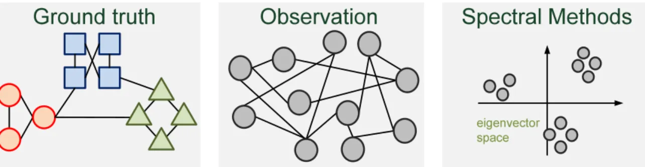
Ground truth
Observation
Spectral Methods
eigenvector space
Figure 1.2: An illustration of graph spectral decomposition methods for graph clus-tering. Graph spectral decomposition methods transform the observed graph into a representation in a low-dimensional vector space to reveal the ground-truth clusters.
K-dimensional vectors or degree normalization of the adjacency matrix can be used to stabilize K-means clustering [97,108,176]. Fig. 1.2 illustrates the methodology of graph spectral decomposition methods for graph clustering, which includes spectral clustering. Graph spectral decomposition methods transform the observed graph into a representation in a low-dimensional vector space to reveal the ground-truth clusters. The success of spectral clustering can be explained by the fact that acquiring K
smallest eigenvectors of L is equivalent to solving a relaxed graph cut minimization problem, which partitions a graph into K clusters by minimizing various objective functions including min cut, ratio cut or normalized cut [97].
1.4
Overview of Graph Clustering Methods
Broadly speaking, actions on graphs can be viewed as various means for optimizing an objective function associated with a data analysis task. For graph clustering, the fundamental task is to partition the nodes in a graph into groups based on the graph connectivity structure. Different graph clustering methods lead to different edge removal strategies that uncover the cluster structures, and the associated cost often relates to the total edge weight of the removed edges, which is known as the min-cut score. In particular, one principal method for graph clustering is through graph spectral decompositions.
Throughout this dissertation we will use the terms “graph clustering” and “com-munity detection” interchangeably, as they both aim at clustering nodes in a graph but may target different objective functions based on the data features, e.g., a simi-larity graph of an image, or a friendship graph of a social network.
1.4.1 Graph clustering methods and analysis for single-layer graphs
Graph clustering has been an active research field across various disciplines, in-cluding machine learning, physics, data mining, graph signal processing, computer science, bio-informatics, network analysis, and data science. Here we categorize the related work based on the methodologies for graph clustering. Interested readers can refer to the [56] and the references therein for more details.
Spectral algorithms. In principle, spectral algorithms utilize the eigenstruc-ture of matrices associated with the graph data for clustering. For instance, spectral clustering [97, 108, 166, 176] uses the graph Laplacian matrix, the spectral modularity method [105, 106] uses the modularity matrix, and the spectral redemption method [87, 139] uses the nonbacktracking matrix.
Inference methods. Inference methods are built upon generative network models such as the stochastic block model (SBM) [74] and its variants [4]. The task is to infer the cluster assignment for each node based on the graph connectivity structure. In [80], the authors infer clusters based on a maximum likelihood method. Other methods such as belief propagation and message passing are proposed in [47, 73,179].
Hierarchical methods. Hierarchical methods can often relate to clustering based on dendrograms. Popular methods for creating dendrograms include re-moving edges of high betweenness measure [63], greedy modularity maximiza-tion approaches [18,104], label propagation [135], and node removals based on
centrality measures [165].
Random walk based methods. Random walk based methods specify a tran-sition matrix of random walks on a graph and use its stationary distribution of random walks for clustering. Typical methods can be found in [125, 160]. Performance limits for graph clustering. Recently there is growing interest
in understanding the universal limits of graph clustering, as well as performance limits of specific graph clustering methods. Most of the works assume the graph data is a realization of a generative network model, such as the SBM [181]. For instance, the performance limit of the spectral modularity method is studied in [102], the performance limit of eigenspectrum-based approaches is studied in [122], and the information theoretic limit is studied in [1]. A summary of inferential limits under the SBM can be found in [2].
1.4.2 Model order selection
A long-standing challenge for graph clustering is the selection of cluster counts K
for partitioning. For spectral clustering, it is equivalent to selecting the number K
of smallest eigenvectors of L that best fits the data, which we call it as the model order selection problem. Most existing model selection algorithms specify an upper boundKmaxon the numberK of clusters and then selectK based on optimizing some
objective function, e.g., the goodness of fit of thek-cluster model fork = 2, . . . , Kmax.
In [108], the objective is to minimize the sum of cluster-wise Euclidean distances between each data point and the centroid obtained from K-means clustering. In [124], the objective is to maximize the gap between theK-th largest and the (K+ 1)-th largest eigenvalue. In [176], 1)-the au1)-thors propose to minimize an objective function that is associated with the cost of aligning the eigenvectors with a canonical coordinate system. A model based method for determining the number of clusters is proposed
in [126]. In [105], the authors propose to iteratively divide a cluster based on the leading eigenvector of the modularity matrix until no significant improvement in the modularity measure can be achieved. The Louvain method in [18] uses a greedy algorithm for modularity maximization. In [87, 139], the authors propose to use the eigenvectors of the nonbacktracking matrix for graph clustering, where the number of clusters is determined by the number of real eigenvalues with magnitude larger than the square root of the largest eigenvalue.
1.4.3 Graph clustering methods and analysis for multilayer graphs
Graph clustering on multilayer graphs aims to find a consensus cluster assignment on each node in the common node set shared by different layers. Layer aggregation has been a principal method for processing and mining multilayer graphs [20,46,153, 154, 156, 168], as it transforms a multilayer graph into a single aggregated graph, facilitating application of data analysis techniques designed for single-layer graphs. Extending from the stochastic block model (SBM) for graph clustering in single-layer graphs [74], multilayer SBM has been proposed for graph clustering on multilayer graphs [10,71,121,149,156,159]. Under the assumption of two equally-sized clusters, the authors in [156] show that if each layer is an independent realization of a common SBM, the inferential limit for cluster detectability decays with O(L−12), where L
is the number of layers. In [149], a layer selection method based on a multilayer SBM is proposed to improve the performance of graph clustering by identifying a subset of layers of a common SBM. However, multilayer SBM assumes homogeneous connectivity structure for within-cluster and between-cluster edges in each layer, and it assumes layer-wise independence.
In addition to inference approaches based on multilayer SBM, other methods have been proposed for graph clustering on multilayer graphs, including information-theoretic approaches [77, 117], k-nearest neighbor method [67], nonnegative matrix
factorization [110], flow-based approach [45], linked matrix factorization [155], random walk [89], tensor decomposition [43], subspace methods [51,52], and greedy multilayer modularity maximization [101]. More details on multilayer graph models can be found in the recent surveys on graph clustering on multilayer graphs [81,84].
It is worth mentioning that the aforementioned work requires the knowledge of the number of clusters (model order) for graph clustering, especially for matrix decomposition-based methods [43,51,52,110, 155] and multilayer SBM [10,71, 121, 149, 156, 159]. However, in many practical cases the model order is not known in advance. Although many model order selection methods have been proposed for auto-mated graph clustering without prespecifying the model order for single-layer graphs [18, 31, 87, 176], little has been developed for automated model order selection for graph clustering on multilayer graphs. Moreover, many layer aggregation methods assign uniform weights over layers such that the aggregated graph is insensitive to the quality of clusters in each layer [153, 154,156].
1.5
Overview of Node Centrality Measures
Node and edge centralities are quantitative measures that are used to evaluate the level of importance and/or influence of a node or an edge in the network. Centrality measures can be classified into two categories, global and local measures. Global centrality measures require complete topological information for their computation, whereas local centrality measures only require partial topological information from neighboring nodes. For instance, acquiring shortest path information between every node pair is a global method required for the betweenness centrality measure, and acquiring degree information of every node is a local method. Some commonly used centrality measures are:
pass-ing through a node relative to the total number of shortest paths in the net-work. Specifically, betweenness is a global measure defined as betweenness(i) =
P
k6=i
P
j6=i,j>k φkj(i)
φkj , where φkj is the total number of shortest paths from k to
j and φkj(i) is the number of such shortest paths passing through i. A similar notion is used to define the edge betweenness centrality [63].
Closeness [140]: closeness is a global measure of geodesic distance of a node to all other nodes. A node is said to have high closeness if the sum of its shortest path distances to other nodes is small. Let ρ(i, j) denote the shortest path distance between nodeiand node j in a connected graph. Then we define closeness(i) = 1/P
j∈V,j6=iρ(i, j).
Eigenvector centrality (eigen centrality) [107]: eigenvector centrality is the
i-th entry of the eigenvector associated with the largest eigenvalue of the adja-cency matrixA. It is defined as eigen(i) =λ−max1 P
j∈VWjiξj, whereλmaxis the
largest eigenvalue ofAandξ is the left eigenvector associated withλmax. It is a
global measure since eigenvalue decomposition of A requires global knowledge of the graph topology.
Degree (di): degree is the simplest local node centrality measure which ac-counts for the number of neighboring nodes.
Ego centrality [54]: consider the (di+ 1)-by-(di+ 1) local adjacency matrix of nodei, denoted by A(i), and let R be a matrix of ones. Ego centrality can be viewed as a local version of betweenness that computes the shortest paths be-tween its neighboring nodes. Since [A2(i)]
kj is the number of two-hop walks be-tweenkandj, andhA2(i)◦ E−A(i)i
kj
is the total number of two-hop short-est paths betweenk andj for allk 6=j, where◦denotes entrywise matrix prod-uct. Ego centrality is defined as ego(i) =P
k P j>k1/ h A2(i)◦ E−A(i)i kj.
Chapters Graph spectral decompositions Insertions/Removals of nodes/edges I II X III X IV X V X VI X VII X X VIII X X IX X X X X X XI
Table 1.1: Dissertation outline with respect to two actions on graphs
1.6
Dissertation Outline and Contributions
The dissertation outline with respect to two actions on graphs, graph spectral decompositions and insertions and removals of nodes or edges, is listed in Table 1.1. The contributions of each chapter are summarized as follows.
Chapter II proposes an efficient incremental eigenpair computation method for graph Laplacian matrices. The proposed method adapts a novel matrix trans-form that enables fast incremental eigenpair computation of increasing eigenpair orders. In particular, the proposed method significantly outperforms the batch computation method in terms of computation time. This incremental eigen-pair computation method can be readily applied to iterative graph clustering of increasing orders in the following chapters.
Chapter III establishes phase transition analysis of the spectral modularity method under the stochastic block model (SBM) with K = 2 clusters. The phase transition results are shown to be universal in the sense that the critical threshold affecting the performance of spectral modularity method is indepen-dent of the clusters sizes as long as they grow with comparable rates.
(SGC) under the random interconnection model (RIM). The analysis identifies the role of inter-cluster edge connection probabilities in the success of SGC. Specifically, we show that under the RIM, a graph can be separated into two regimes: a regime where SGC is successful, and a regime where SGC is un-successful. It is called a phase transition since the regimes are separated by a critical value of the inter-cluster inter-cluster edge connection probability. The phase transition analysis is then extended to undirected weighted graphs gen-erated by the RIM.
Chapter V develops an automated model order selection (AMOS) algorithm for determining the number of clusters in single-layer weighted graphs based on the phase transition analysis established in Chapter IV. AMOS works by iterative spectral graph clustering of increasing model orders, and finds the minimal model order such that the identified clusters meet the phase transition criterion for clustering reliability. AMOS also provides statistical clustering reliability guarantees for graph data inference. Experimental results on several real-life datasets show that AMOS can produce consistent clusters when compared with the meta information, e.g., ground-truth clusters or geographical separations. Chapter VI establishes phase transition analysis of spectral graph clustering in
multi-layer graphs via convex layer aggregation. Based on the phase transition analysis, a multilayer iterative model order selection algorithm (MIMOSA) is proposed for model selection and layer weight adaption for graph clustering in multilayer graphs with statistical clustering reliability. The success of MIMOSA can be explained by a multilayer signal plus noise model since its layer weight adaption process is sensitive to the noise level of each layer.
Chapter VII introduces a new centrality measure called local Fielder vector cen-trality (LFVC). Stemming from algebraic connectivity minimization via node/edge
removals, LFVC evaluates the importance of a node or an edge for graph con-nectivity. In particular, we show that greedy node removals based on LFVC have bounded performance guarantee relative to the optimal batch removals. Based on LFVC removals, a deep community detection algorithm is proposed to extract important communities from the graph.
Chapter VIII proposes a method for identifying influential links for event prop-agation on Twitter, also applicable to other social network applications, where the influence of a link is evaluated in terms of the effect of its removal on event propagation. The proposed method incorporates the network of networks structure embedded in Twitter follower networks, and can effectively identify influential links in several actual event propagation traces.
Chapter IX proposes an edge rewiring algorithm for enhancing network re-silience to centrality attacks. The proposed method works by swapping edges in the graph for improved algebraic connectivity without introducing additional edges, and it can be implemented in a distributed fashion. Experimental results on real-like network show that the proposed method can effectively enhance the network resilience by only rewiring a few edges in the graph.
Chapter X develops a graph-theoretic framework for cyber resilience against lateral movement attacks. By modeling the interactions among user, hosts, and applications in an enterprise network as a tripartite heterogeneous graph and mapping feasible preventative actions to operations on the associated graph ma-trices, we propose greedy algorithms with performance guarantees to enhance enterprise cyber resiliency. Experimental results show that the proposed meth-ods can greatly contain simulated lateral movement attacks in actual enterprise networks and actual lateral movement attacks extracted from real-world traces.
1.7
List of Relevant Publications
1.7.1 Journal publications
P.-Y. Chen and A. O. Hero, “Deep Community Detection,”IEEE Transactions on Signal Processing, vol. 63, no. 21, pp. 5706-5719, Nov. 2015 [24]
P.-Y. Chen and A. O. Hero, “Phase Transitions in Spectral Community Detec-tion,”IEEE Transactions on Signal Processing, vol. 63, no. 16, pp. 4339-4347, Aug. 2015 [25]
P.-Y. Chen and A. O. Hero, “Universal Phase Transition in Community De-tectability under a Stochastic Block Model,” Physical Review E, vol. 91, no.3, pp. 032804, Mar. 2015 [29]
P.-Y. Chen and A. O. Hero, “Assessing and Safeguarding Network Resilience to Nodal Attacks,”IEEE Communications Magazine, vol. 52, no. 11, pp. 138-143, Nov. 2014 [27]
1.7.2 Conference publications
P.-Y. Chen and A. O. Hero, “Multilayer Spectral Graph Clustering via Convex Layer Aggregation,” IEEE Global Conference on Signal and Information Pro-cessing (GlobalSIP), Dec. 2016
P.-Y. Chen, B. Zhang, M. Hasan and A. O. Hero, “Incremental Method for Spectral Clustering of Increasing Orders,” ACM SIGKDD International Con-ference on Knowledge Discovery and Data Mining (KDD) Workshop on Mining and Learning with Graphs (MLG), Aug. 2016 [36]
P.-Y. Chen, S. Choudhury, and A. O. Hero, “Multi-Centrality Graph Spectral Decompositions and Their Application to Cyber Intrusion Detection,”IEEE In-ternational Conference on Acoustics, Speech and Signal Processing (ICASSP),
pp. 4553-4557, Mar. 2016 [34]
P.-Y. Chen and A. O. Hero, “Phase Transitions in Spectral Community Detec-tion of Large Noisy Networks,” IEEE International Conference on Acoustics, Speech and Signal Processing (ICASSP), pp. 3402-3406, Apr. 2015 [30]
P.-Y. Chen and A. O. Hero, “Local Fiedler Vector Centrality for Detection of Deep and Overlapping Communities in Networks,” IEEE International Con-ference on Acoustics, Speech and Signal Processing (ICASSP), pp. 1120-1124, May 2014 [28]
P.-Y. Chen and A. O. Hero, “Node Removal Vulnerability of the Largest Com-ponent of a Network,”IEEE Global Conference on Signal and Information Pro-cessing (GlobalSIP), pp. 587-590. Dec. 2013 [26]
1.7.3 Submitted papers
P.-Y. Chen and A. O. Hero, “Multilayer Spectral Graph Clustering via Convex Layer Aggregation: Theory and Algorithm,” 2016
P.-Y. Chen, C.-C. Tu, P.-S. Ting, Y.-Y. Luo, D. Koutra, and A. O. Hero, “Iden-tifying Influential Links for Event Propagation on Twitter: A Network of Net-works Approach,” 2016 [35]
P.-Y. Chen, Thibaut Gensollen, and A. O. Hero, “AMOS: An Automated Model Order Selection Algorithm for Spectral Graph Clustering,” 2016
P.-Y. Chen, S. Sutanay, L. Rodriguez, A. O. Hero, and I. Ray, “Enterprise Cy-ber Resiliency Against Lateral Movement: A Graph Theoretic Approach,” 2016 P.-Y. Chen and A. O. Hero, “Phase Transitions and a Model Order Selection
CHAPTER II
Incremental Method for Spectral Graph
Clustering of Increasing Orders
As introduced in Chapter I, the smallest eigenvalues and the associated eigen-vectors (i.e., the smallest eigenpairs) of a graph Laplacian matrix have been widely used for spectral clustering and community detection. However, the majority of ap-plications require computation of a large number Kmax of eigenpairs, where Kmax
is an upper bound on the number K of clusters, called the order of the clustering algorithms. In this chapter, we propose an incremental method for constructing the eigenspectrum of the graph Laplacian matrix. This method leverages the eigenstruc-ture of graph Laplacian matrix to obtain the (k+ 1)-th eigenpairs of the Laplacian matrix given a collection of all the k smallest eigenpairs. Our proposed method adapts the Laplacian matrix such that the batch eigenvalue decomposition problem transforms into an efficient sequential leading eigenpair computation problem.
Generally, the number of clusters K is selected to be much smaller than n (the number of data points), making full eigen decomposition (such as QR decomposition) unnecessary. An efficient alternative is to use methods that are based on power iteration, such as Arnoldi method or Lanczos method, which computes the leading eigenpairs through repeated matrix vector multiplication. ARPACK [94] library is a popular parallel implementation of different variants of Arnoldi and Lanczos method,
which is used by many commercial software including Matlab.
However, in most situations the best value ofKis unknown and a heuristic is used by clustering algorithms to determine the number of clusters, e.g., fixing a maximum number of clusters Kmax and detecting a large gap in the values of the Kmax largest
sorted eigenvalues or normalized cut score [108, 124]. Alternatively, this value of K
can be determined based on domain knowledge [11]. For example, a user may require that the largest cluster size be no more than 10% of the total number of nodes or that the total inter-cluster edge weight be no greater than a certain amount. In these cases, the desired choice of K cannot be determineda priori. Over-estimation of the upper bound Kmax on the number of clusters is expensive as the cost of finding K
eigenpairs using the power iteration method grows rapidly with K. On the other hand, choosing an insufficiently large value for Kmax runs the risk of severe bias.
SettingKmax to the number of data points n is generally computationally infeasible,
even for a moderate-sized graph. Therefore, an incremental eigenpair computation method that effectively computes the K-th smallest eigenpair of graph Laplacian matrix by utilizing the previously computed K − 1 smallest eigenpairs is needed. Such an iterative method obviates the need to set an upper bound Kmax on K, and
its efficiency can be explained by the adaptivity to increments in K.
In this chapter, we propose an efficient method for incremental computation of smallest eigenpairs by exploiting the eigenspace structure of graph Laplacian ma-trices. For each increment, given the previously computed smallest eigenpairs, we show that computing the next smallest eigenpair is equivalent to computing a lead-ing eigenpair of a particular matrix, which transforms potentially tedious numerical computation (such as the tridiagonalization step in Lanczos algorithm [90]) to simple matrix power iterations of known computational efficiency [90]. Our experimental results show that for a given K, the proposed incremental computation provides a significant reduction in computation time compared to a batch computation method
which computes the K smallest eigenpairs in a single batch. Also, as K increases, the gap between the incremental approach and the batch approach widens, providing an order of magnitude speed-up.
It is worth noting that the proposed method aims to incrementally compute the smallest eigenpair of a given graph Laplacian matrix. There are several works that are named as incremental eigenvalue decomposition methods [50, 79, 111, 112, 136]. However, these works focus on updating the eigenstructure of graph Laplacian matrix of dynamic graphs when nodes (data samples) or edges are inserted or deleted into the graph.
2.1
Incremental Eigenpair Computation for Graph Laplacian
Matrices
2.1.1 Notation for eigenpairs
The i-th smallest eigenvalue and its associated unit-norm eigenvector of L are denoted by λi(L) and vi(L), respectively. That is, the eigenpair (λi,vi) of L has the relation Lvi = λivi, and λ1(L) ≤ λ2(L) ≤ . . . ≤ λn(L). The eigenvectors have unit Euclidean norm and they are orthogonal to each other such that vT
i vj = 1 if i = j and vT
i vj = 0 if i 6= j. The eigenvalues of L are said to be distinct if
λ1(L)< λ2(L)< . . . < λn(L). Similar notation is used for LN.
2.1.2 Theoretical foundations of the proposed method
The following lemmas and corollaries provide the cornerstone for establishing the incremental computation method. The main idea is that we utilize the eigenspace structure of graph Laplacian matrix to inflate specific eigenpairs via a particular per-turbation matrix, without affecting other eigenpairs. The proposed method can be viewed as a specialized Hotelling’s deflation method [118] designed for graph
Lapla-Type / Graph Laplacian Unnormalized Normalized
Connected Graphs Lemma 2.1, Theorem 2.6 Corollary 2.2, Corollary 2.8 Disconnected Graphs Lemma 2.3, Theorem 2.7 Corollary 2.4, Corollary 2.9 Table 2.1: Utility of the established lemmas, corollaries, and theorems in Chapter II. cian matrices by exploiting their spectral properties and associated graph character-istics. It works for both connected, and disconnected graphs using both normalized and unnormalized graph Laplacian matrices. For illustration purposes, in Table 2.1 we group the established lemmas, corollaries, and theorems under different graph types and different graph Laplacian matrices. The proofs of the established lemmas, theorems and corollaries are given in Appendix A.
Lemma 2.1. Assume thatG is a connected graph and L is the graph Laplacian with si denoting the sum of the entries in the i-th row of the weight matrix W. Let s =
Pn
i=1si and defineLe =L+ns1n1Tn. Then the eigenpairs of Le satisfy (λi(Le),vi(Le)) =
(λi+1(L),vi+1(L)) for 1≤i≤n−1 and (λn(Le),vn(Le)) = (s,√1n
n).
Corollary 2.2. For a normalized graph Laplacian matrix LN, assume G is a
con-nected graph and letLeN =LN+2sS
1 21n1T nS 1 2. Then(λi(LeN),vi(LeN)) = (λi+1(LN),vi+1(LN)) for 1≤i≤n−1 and (λn(LeN),vn(LeN)) = (2,S 1 21n √ s ).
Lemma 2.3. Assume that G is a disconnected graph with δ ≥ 2 connected compo-nents, and lets=Pn
i=1si, let V= [v1(L),v2(L), . . . ,vδ(L)], and letLe =L+sVVT.
Then (λi(Le),vi(Le)) = (λi+δ(L),vi+δ(L)) for1≤i≤n−δ, λi(Le) =s for n−δ+ 1≤
i≤n, and [vn−δ+1(Le),vn−δ+2,(Le),
. . . ,vn(Le)] =V.
Corollary 2.4. For a normalized graph Laplacian matrix LN, assume Gis a
discon-nected graph withδ≥2connected components. LetVδ = [v1(LN),v2(LN), . . . ,vδ(LN)],
and let LeN =LN + 2VδVδT. Then (λi(LeN),vi(LeN)) = (λi+δ(LN),vi+δ(LN)) for 1≤
i≤n−δ,λi(LeN) = 2forn−δ+1≤i≤n, and[vn−δ+1(LeN),vn−δ+2,(LeN), . . . ,vn(LeN)] =
Remark 2.5. The columns of any matrix V0 = VR with an orthonormal transfor-mation matrix R (i.e., RTR=I) are also the largest δ eigenvectors of
e
L and LeN in
Lemma 2.3 and Corollary 2.4. Without loss of generality we consider the caseR=I.
2.1.3 Incremental eigenpair computation method
Given the K smallest eigenpairs of a graph Laplacian matrix, we prove that com-puting the (K+ 1)-th smallest eigenpair is equivalent to computing the leading eigen-pair (the eigeneigen-pair with the largest eigenvalue in absolute value) of a certain perturbed matrix. The advantage of this transformation is that the leading eigenpair can be efficiently computed via matrix power iteration methods [90,94].
Let VK = [v1(L),v2(L), . . . ,vK(L)] be the matrix with columns being the K smallest eigenvectors ofLand letΛK = diag(s−λ1(L), s−λ2(L), . . . , s−λK(L)) be the diagonal matrix with {s−λi(L)}Ki=1 being its main diagonal. The following theorems
show that given the K smallest eigenpairs ofL, the (K + 1)-th smallest eigenpair of
L is the leading eigenvector of the original graph Laplacian matrix perturbed by a certain matrix.
Theorem 2.6. (connected graphs)GivenVK andΛK, assume thatG is a connected
graph. Then the eigenpair (λK+1(L),vK+1(L)) is a leading eigenpair of the matrix e
L =L+VKΛKVKT + s n1n1
T
n −sI. In particular, if L has distinct eigenvalues, then (λK+1(L),vK+1(L)) = (λ1(Le) +s,v1(Le)).
The next theorem describes an incremental eigenpair computation method when the graph G is a disconnected graph with δ connected components. The columns of the matrix Vδ are the δ smallest eigenvectors of L. Note that Vδ has a canonical representation where the nonzero entries of each column are a constant and their indices indicate the nodes in each connected component [26, 97], and the columns of
Vδ are the δ smallest eigenvectors of L with eigenvalue 0 [26]. Since the δ smallest eigenpairs with the canonical representation are trivial by identifying the connected


![Figure 6.3: Phase transitions in the geometric mean of cluster detectability from multilayer SGC via convex layer aggregation for the two-layer correlated graph model, where w 1 is uniformly sampled from the [0, 1] with unit interval 0.1](https://thumb-us.123doks.com/thumbv2/123dok_us/1440687.2692938/112.918.262.637.144.469/transitions-geometric-detectability-multilayer-aggregation-correlated-uniformly-interval.webp)
![Figure 6.4: The effect of the layer weight vector w = [w 1 w 2 ] T on the accuracy of multilayer SGC with respect to difference noise level {p (`) } 2 `=1 for the two-layer correlated graph model](https://thumb-us.123doks.com/thumbv2/123dok_us/1440687.2692938/113.918.227.761.212.709/figure-effect-weight-accuracy-multilayer-respect-difference-correlated.webp)